Correlated percolation and tricriticality

Abstract

The recent proliferation of correlated percolation models—models where the addition of edges/vertices is no longer independent of other edges/vertices—has been motivated by the quest to find discontinuous percolation transitions. The leader in this proliferation is what is known as explosive percolation. A recent proof demonstrates that a large class of explosive percolation-type models does not, in fact, exhibit a discontinuous transition[O. Riordan and L. Warnke, Science, 333, 322 (2011)]. We, on the other hand, discuss several correlated percolation models, the $k$-core model on random graphs, and the spiral and counter-balance models in two-dimensions, all exhibiting discontinuous transitions in an effort to identify the needed ingredients for such a transition. We then construct mixtures of these models to interpolate between a continuous transition and a discontinuous transition to search for a tricritical point. Using a powerful rate equation approach, we demonstrate that a mixture of $k=2$-core and $k=3$-core vertices on the random graph exhibits a tricritical point. However, for a mixture of $k$-core and counter-balance vertices, heuristic arguments and numerics suggest that there is a line of continuous transitions as the fraction of counter-balance vertices is increased from zero with the line ending at a discontinuous transition only when all vertices are counter-balance. Our results may have potential implications for glassy systems and a recent experiment on shearing a system of frictional particles to induce what is known as jamming.

I Introduction

Percolation is the study of connected structures in disordered networks percolation1 . For example, two edges meeting at a vertex form a connected structure called a cluster of size two. As more edges are randomly and independently added to the network, the average cluster size grows until there ultimately exists a spanning cluster in finite-dimensional lattices (or a giant component in random graphs). The onset of a spanning cluster, which is indicative of a transition from a non-spanning to spanning phase, exhibits properties of a continuous phase transition. The simplicity of this nontrivial model allows one to catalog many of its properties such that it is the Ising model of geometrically-driven phase transitions percolation2 ; percolation3 .

While the simplicity of percolation is part of its power, there has been a recent renaissance in developing models beyond ordinary percolation in an effort to discover new types of transitions such as a discontinuous one. The main driving force behind this endeavor is what is known as explosive percolation explosive science ; Hans ; explosive3 ; explosive4 ; explosive5 . To be specific, two edges are considered at random and the edge that minimizes, for example, the product of the two clusters it joins is then retained and the other discarded, i.e. a choice has been made as to which edge to retain. Initial numerical data for this particular model on random graphs suggested that the percolation transition is discontinuous such that the emergence of the giant component is explosive, hence the term explosive percolation. Because explosive percolation goes beyond ordinary percolation where there is no choice between edges, a different type of transition is not necessarily surprising. However, a recent mathematical proof shows that the transition in this class of models involving choice on random graphs is, in fact, continuous mathematicalexplosive ; network2 .

Other explosive percolation-type models are being investigated for the possibility of a discontinuous transition. For instance, simulations of explosive percolation on finite-dimensional lattices show signs of a discontinuous phase transition Ziff ; Ziff2 . In addition, in light of the recent proof that models involving a choice (Achlitopas processes) on random graphs exhibit a continuous transition, some researchers have begun to study other models beyond ordinary percolation where there exist various constraints on the occupation of edges (and/or vertices). For example, the Bohman-Frieze-Wormald model allows for the addition of an edge provided it participates in a cluster smaller than some prescribed size with the prescribed size being updated as edges are added Bohman-Frieze-Wormald . Recent work suggests a discontinuous transition on random graphs for this model Chen&D'Souza1 ; chen&D'souza2 and even more recent work suggests a similar result on finite-dimensional graphs such as the cubic lattice BohmanFriezeWormaldD'souza .

While work progresses on these more complicated percolation models, perhaps the simplest beyond ordinary percolation model is known as $k$-core percolation CLR ; network1 ; Jen . $k$-core percolation is defined as the following: Each vertex on a graph needs at least k occupied edges; if the constraint is not obeyed, the vertex and the edges attached to it are recursively removed until a stable $k$-core configuration is reached (with every vertex obeying the $k$-core constraint). It turns out that $k$-core percolation on random graphs exhibits a continuous transition for $k\leq 2$ and a discontinuous transition for $k\geq 3$. However, unlike a typical discontinuous transition there exists not one, but several, diverging lengthscales such that the transition is an unusual one.

So there indeed exists discontinuous percolation transitions in mean-field. What about finite-dimensions? It turns out that $k$-core percolation on various finite-dimensional lattices, such as the triangular lattice triangular lattice , either falls into the same universality class as ordinary percolation or does not exhibit a transition (but interesting finite-size effects), i.e. $p_{c}=1$ pc=1 ; dawson , where $p_{c}$ denotes the critical occupation probability. Of course, in high enough dimensions it is conjectured that the $k\geq 3$-core transition becomes discontinuous jen&brooks . While obtaining a discontinuous transition with $k$-core in finite-dimensions has been difficult, a new class of correlated percolation models, dubbed jamming percolation, with constraints more complex than $k$-core, has been recently shown to exhibit a discontinuous transition in finite-dimensions spiralmodel ; commentonspiralmodel ; replytocommentonspiralmodel ; spiralmodel2 . In addition to exhibiting a discontinuous transition, these models also exhibit diverging lengthscales that grow either as a power law or faster than power law such that they, too, are not the garden variety discontinuous transition.

Since there exists percolation models beyond ordinary percolation exhibiting a discontinuous transition, it is possible to construct hybrid models where some fraction of the edges are occupied via ordinary percolation and the remaining edges are occupied via a choice method or some other constrained method. Since ordinary percolation dominates in one limit and the correlated percolation model, which includes explosive percolation, dominates in the other limit, it may be possible to locate a tricritical point bordering the continuous and discontinuous regimes. The proof that explosive percolation is continuous on random graphs removes the possibility of a tricritical point on random graphs using a hybrid of ordinary percolation and explosive percolation. However, the potential for tricriticality in other correlated percolation models is intriguing and remains a possibility. For example, tricriticality has been explored in hybrids of ordinary percolation and explosive percolation in finite-dimensions Ziff'stricrit .

Here, we explore the possibility of tricriticality in (1) a mixture of $k=2$ and $k=3$-core edges on random graphs and (2) a mixture of $k=3$-core edges and jamming percolation edges in two-dimensions. Cellai and collaborators have studied the mixture of $k=2$ and $k=3$-core on locally tree-like graphs and random graphs Cellai . Therefore, we expect agreement between our results obtained using a dynamic rate equation method and theirs Cellai . As for the second case, jamming percolation models are newer so that we will address some of their properties and argue why the search for a tricritical point in such hybrid models may reach a dead end.

While explosive percolation potentially applies to community networks app1 and human protein homology networks app2 , $k$-core percolation may apply to glassy and jamming systems. The Fredrickson-Andersen model Fredrikson-Andersen is a kinetically-constrained model mimicking the caging effect caging effect experiment in glassy dynamics. The onset of a spanning cluster in $k$-core percolation corresponds to the onset of a glass transition in the Fredrickson-Anderson model sbt . Recently, the Fredrickson-Andersen model was extended to incorporate inhomogeneity in the caging dynamics, i.e. some particles are able to break out of their cage if there are less than $k=2$ particles surrounding it, while others require $k=3$ Sellitto . This system exhibits a tricritical point in mean-field as the average value of $k$ is tuned from two to three, the properties of which were investigated by Cellai and collaborators Cellai . As for another application of $k$-core percolation, the $k$-core condition encodes the scalar aspect of the principle of local mechanical stability present in jammed packing. It turns out that the exponents associated with the mean-field $k\geq 3$-core transition are the same exponents as measured in the jamming transition Jen .

The paper is organized as follows. In the next section (Section II), we present our results for a mixture of $k=2$ and $k=3$-core on the random graph. In Section III we address a mixture of $k=3$-core and jamming percolation models in two-dimensions. In Section VI we discuss the implications of our results.

II Hybrid $k$-core on random graphs

II.1 Revisiting the rate equation approach

In 1996, Pittel, Spencer, and Wormald Wormald3authors proved that the $k\geq 3$-core transition on random graphs is discontinuous using rate equations for the $k$-core culling procedure Wormald . This method allows one to easily obtain the discontinuity and we shall review it here as has been done in Ref. Hartmann .

Consider a random graph with $N$ vertices. At each time step, one vertex whose edges is less than $k$ is removed from the graph. The notion of time is given by time step, $t=T/N$, where $T$ is the number of algorithmic steps taken so far. The change in time is given by $\Delta t=1/N$, which becomes continuous when $N\rightarrow\infty$. At time $t$, the number of vertices is $N(T)=(1-t)N$, and the corresponding distribution of connectivity is $P_{z}(t)=N_{z}(T)/N(T)$.

One can write down the expected change for $N_{z}$ in the $(T+1)$th step. It contains two different contributions: 1) The first contribution corresponds to the removed vertex itself. It appears only in the equations for $N_{z}$ with $z<k$. 2) The second contribution is from the neighbors of the removed vertex. The number of its neighbors with connectivity $z=k$ will be decreased by 1, hence the total number of vertices with connectivity $k$ is decreased by 1. The number of its neighbors with connectivity $z=k+1$ will be decreased by 1, too, leading to the total number of vertices with connectivity $k$ increased by 1. Therefore, the equation for the change for $N_{z}$ for all $z$ is:

$$N_{z}(T+1)-N_{z}(T)=-\frac{\chi_{z}P_{z}(t)}{\overline{\chi}}+\frac{\overline{z\chi}}{\overline{\chi}}[-\frac{zP_{z}(t)}{Z(t)}+\frac{(z+1)P_{z+1}(t)}{Z(t)}].$$ (1)

Here, ${\chi}_{z}$ equals one if $z<k$ and zero otherwise. In addition, $\overline{\chi}=\sum_{z}{\chi}_{z}P_{z}(t)$ and $\overline{z\chi}=\sum_{z}z\chi_{z}P_{z}(t)$. The average connectivity is defined as $Z(t)\equiv\overline{z}=\sum_{z}zP_{z}(t)$.

In the thermodynamic limit, the difference equations become differential equations, or

$$\frac{d}{dt}\{(1-t)P_{z}(t)\}=-\frac{\chi_{z}P_{z}(t)}{\overline{\chi}}+\frac{\overline{z\chi}}{\overline{\chi}}[-\frac{zP_{z}(t)}{Z(t)}+\frac{(z+1)P_{z+1}(t)}{Z(t)}].$$ (2)

This infinite set of differential equation is not easy to solve. However, one can assume that as vertices get removed, those who have never been touched, i.e. whose connectivity is greater than $k$, obey Poisson statistics with an effective connectivity ${\beta}(t)$ and initial connectivity ${\beta}(0)=c$. In other words,

$$(1-t)P_{z}(t)=\frac{N_{z}(T)}{N}=e^{-\beta(t)}\frac{\beta(t)^{z}}{z!}\,\,\,\,\,\,\,\,{\forall}z{\geq}k.$$ (3)

With this ansatz, one can write the normalization condition as:

$$1 = \sum_{z=0}^{\infty}P_{z}(t)$$ (4)

$$= \sum_{z=0}^{\infty}\chi_{z}p_{z}(t)+\sum_{z=k}^{\infty}\frac{1}{1-t}e^{-\beta(t)}\frac{\beta(t)^{z}}{z!}$$

$$= \bar{\chi}+\frac{1}{1-t}F_{k}(\beta(t)),$$

where

$$F_{k}(\beta)=1-\sum_{z=0}^{k-1}e^{-\beta(t)}\frac{\beta(t)^{z}}{z!}.$$ (5)

Moreover, the average connectivity, $Z(t)$, can be written as:

$$Z(t) = \sum_{z=0}^{\infty}zP_{z}(t)$$ (6)

$$= \sum_{z=0}^{\infty}z\chi_{z}p_{z}(t)+\sum_{z=k}^{\infty}\frac{z}{1-t}e^{-\beta(t)}\frac{\beta(t)^{z}}{z!}$$

$$= \overline{z\chi}+\frac{\beta(t)}{1-t}F_{k-1}(\beta(t)).$$

Finally, the rate equation becomes,

$$\dot{\beta}(t)=-\frac{\beta(t)}{(1-t)Z(t)}\frac{\overline{z\chi}}{\bar{\chi}}.$$ (7)

One can also obtain

$$(1-t)Z(t)=\frac{\beta^{2}(t)}{c}$$ (8)

by comparing $\dot{\beta}(t)$ and $\frac{d}{dt}((1-t)Z(t))$ with the latter obtained using the rate equation.

Now, the culling procedure ends when the graph reaches a stable $k$-core configuration. In other words, when $\overline{\chi}=\overline{z\chi}=0$ for all $z{\geq}k$. Therefore, Eq. 5 and Eq. 6 simplify to

$$1-t_{f} = F_{k}(\beta_{f})$$

$$\frac{\beta_{f}}{c} = F_{k-1}(\beta_{f}),$$ (9)

where $\beta_{f}=\beta(t_{f})$ and we have used Eq. 8. To study the nature of the transition, for a given $c$ (or initial occupation probability $c=p/N$), one solves for $\beta_{f}$ using the second equation and then computes $1-t_{f}$, which yields the fraction of vertices left and is of the order of the giant component should it exist. For $k=2$, the critical initial concentration signalling the onset of the giant component is $c_{q}=1$. For $c=c_{g}+\epsilon$ with $\epsilon<<1$, $1-t_{f}=2\epsilon^{2}+\mathcal{O}(\epsilon^{3})$, i.e. the transition is continuous. For $k=3$, $1-t_{f}$ is finite at the transition such that the transition is discontinuous.

II.2 Hybrid model of $k=2$-core and $k=3$-core

To search for a tricritical point, we define a model where some fraction of $k=k_{1}$ vertices, $f$, and the remaining fraction as $k=k_{2}$ vertices. In this model, normalization demands that

$$1 = \sum_{z=0}^{\infty}P_{z}(t)$$ (10)

$$= f\sum_{z=0}^{\infty}P_{z}(t)+(1-f)\sum_{z=0}^{\infty}P_{z}(t)$$

$$= f(\sum_{z=0}^{k_{1}-1}P_{z}(t)+\sum_{z=k_{1}}^{\infty}P_{z}(t))+(1-f)(\sum_{z=0}^{k_{2}-1}P_{z}(t)+\sum_{z=k_{2}}^{\infty}P_{z}(t))$$

As before, we will assume that for the $k_{1}$-core vertices, as long as $z\geq k_{1}$, their Poissonian structure is retained with some effective connectivity that changes as a function of time. We will assume this property for the $k_{2}$-core vertices as well with both types of vertices having the same effective connectivity since they are part of the same graph. Therefore,

$$1=f(\sum_{z=0}^{\infty}\chi_{k_{1}}P_{z}(t)+\sum_{z=k_{1}}^{\infty}\frac{1}{1-t}e^{-\beta(t)}\frac{\beta(t)^{d}}{d!})+(1-f)(\sum_{z=0}^{\infty}\chi_{k_{2}}P_{z}(t)+\sum_{z=k_{2}}^{\infty}\frac{1}{1-t}e^{-\beta(t)}\frac{\beta(t)^{z}}{z!}),$$ (11)

where $\chi_{k_{1}}$ applies to the $k_{1}$-core vertices with $\chi_{k_{1}}=0$ for $z\geq k_{1}$ and is unity otherwise, and similarly, for $\chi_{k_{2}}$ with $k_{2}$ replacing $k_{1}$, to arrive at

$$1=f\overline{\chi_{k_{1}}}+\frac{1}{1-t}F_{k_{1}}(\beta(t))+(1-f)(\overline{\chi_{k_{2}}}+\frac{1}{1-t}F_{k_{2}}(\beta(t))).$$ (12)

Moreover, the average connectivity can be written as:

$$Z(t)=f(\overline{z\chi_{k_{1}}}+\frac{\beta(t)}{1-t}F_{k_{1}-1}(\beta(t)))+(1-f)(\overline{z\chi_{k_{2}}}+\frac{\beta(t)}{1-t}F_{k_{2}-1}(\beta(t))).$$ (13)

We, again, use the rate equation to obtain a relation between the average connectivity and the effective connectivity. The rate equation for the hybrid model is

$$\frac{d}{dt}\{(1-t)P_{z}(t)\}=f\{-\frac{\chi_{k_{1}}P_{z}(t)}{\overline{\chi_{k_{1}}}}+\frac{\overline{z\chi_{k_{1}}}}{\overline{\chi_{k_{1}}}}[-\frac{zP_{z}(t)}{Z(t)}+\frac{(z+1)P_{z+1}(t)}{Z(t)}]\}+(1-f)\{-\frac{\chi_{k_{2}}P_{z}(t)}{\overline{\chi_{k_{2}}}}+\frac{\overline{z\chi_{k_{2}}}}{\overline{\chi_{k_{2}}}}[-\frac{zP_{z}(t)}{Z(t)}+\frac{(z+1)P_{z+1}(t)}{Z(t)}]\}.$$ (14)

Using the Possionian ansatz, the RHS of the rate equation becomes

$$f\frac{\overline{z\chi_{k_{1}}}}{\overline{\chi_{k_{1}}}}[-e^{-\beta(t)}\frac{\beta(t)^{z}}{(z-1)!(1-t)Z(t)}+e^{-\beta(t)}\frac{\beta(t)^{z+1}}{z!(1-t)Z(t)}]$$ (15)

$$+ (1-f)\frac{\overline{z\chi_{k_{2}}}}{\overline{\chi_{k_{2}}}}[-e^{-\beta(t)}\frac{\beta(t)^{z}}{(z-1)!(1-t)Z(t)}+e^{-\beta(t)}\frac{\beta(t)^{z+1}}{z!(1-t)Z(t)}],$$

and the LHS is

$$\dot{\beta(t)}[e^{-\beta(t)}\frac{\beta(t)^{z-1}}{(z-1)!}-e^{-\beta(t)}\frac{\beta(t)^{z}}{z!}]$$ (16)

to arrive at

$$\dot{\beta(t)}=-\frac{\beta(t)}{m(t)}(f\frac{\overline{z\chi_{k_{1}}}}{\overline{\chi_{k_{1}}}}+(1-f)\frac{\overline{z\chi_{k_{2}}}}{\overline{\chi_{k_{2}}}}),$$ (17)

where $m(t)=(1-t)Z(t)$. It turns out that

$$\dot{m(t)} = \frac{d}{dt}\{(1-t)\sum_{z}zP_{z}(t)\}$$ (18)

$$= \sum_{z}z\frac{d}{dt}\{(1-t)P_{z}(t)\}$$

$$= -f\frac{\overline{z\chi_{k_{1}}}}{\overline{\chi_{k_{1}}}}+f\frac{\overline{z\chi_{k_{1}}}}{\overline{\chi_{k_{1}}}}[-\frac{\overline{z^{2}}}{Z(t)}+\frac{\overline{z(z-1)}}{Z(t)}]-(1-f)\frac{\overline{z\chi_{k_{2}}}}{\overline{\chi_{k_{2}}}}+(1-f)\frac{\overline{z\chi_{k_{2}}}}{\overline{\chi_{k_{2}}}}[-\frac{\overline{z^{2}}}{Z(t)}+\frac{\overline{z(z-1)}}{Z(t)}]$$

$$= -2(f\frac{\overline{z\chi_{k_{1}}}}{\overline{\chi_{k_{1}}}}+(1-f)\frac{\overline{z\chi_{k_{2}}}}{\overline{\chi_{k_{2}}}})$$

such that

$$\frac{\dot{\beta}(t)}{\beta(t)}=\frac{1}{2}\frac{\dot{m}(t)}{m(t)}$$ (19)

whose solution is $m(t)=\frac{\beta^{2}(t)}{c}$ as before.

Now we are ready to extract the criticial behavior for this hybrid model by occupying edges at random with an initial average connectivity $Z(0)=c$ and iterating the culling process until a stable configuration is found at time $t=t_{f}$. Given the $k$-core constraints, when $t=t_{f}$, $\overline{\chi_{k_{1}}}=\overline{\chi_{k_{2}}}=\overline{z\chi_{k_{1}}}=\overline{z\chi_{k_{2}}}=0$ such that the normalization condition becomes

$$1=f\sum_{z=k_{1}}^{k_{2}-1}\frac{1}{1-t_{f}}e^{-\beta_{f}}\frac{\beta_{f}^{z}}{z!}+\sum_{z=k_{2}}^{\infty}\frac{1}{1-t_{f}}e^{-\beta_{f}}\frac{\beta_{f}^{z}}{z!}$$ (20)

with $\beta_{f}=\beta(t_{f})$. The average connectivity equation becomes

$$Z(t_{f})=f\sum_{z=k_{1}}^{k_{2}-1}\frac{z}{1-t_{f}}e^{-\beta_{f}}\frac{\beta_{f}^{z}}{z!}+\beta_{f}\frac{1}{1-t_{f}}F_{k_{2}-1}(\beta_{f}).$$ (21)

For $k_{1}=2$ and $k_{2}=3$,

$$Z(t_{f})=\frac{2f}{1-t_{f}}e^{-\beta_{f}}\frac{\beta_{f}^{2}}{2}+\frac{\beta_{f}}{1-t_{f}}(1-e^{-\beta_{f}}(1+\beta_{f})).$$ (22)

Using Eq. 8, we arrive at

$$\frac{\beta_{f}}{c}=fe^{-\beta_{f}}\beta_{f}+1-e^{-\beta_{f}}(1+\beta_{f})=F(\beta_{f}).$$ (23)

As before, this self-consistency equation determines $\beta_{f}$ and then one can use the normalization condition at $t=t_{f}$ to find the size of the giant component. See Figures 1-3 for a graphical representation of this equation for different values of $f$.

When $f=1$, the model reduces to $k=2$-core, and the transition is continuous. When $f=0$, the model reduces to $k=3$-core, and the transition is discontinuous. As $f$ is varied between zero and unity, the curvature of $F(\beta_{f})$ at $\beta_{f}=0$ changes from positive to negative such that for some particular value of $f$, the curvature of $F(\beta_{f})$ at $\beta_{f}=0$ vanishes. In other words, there exists a tricritical point separating the continuous $k=2$-core transition from the discontinuous $k=3$-core transition. This tricritical point occurs at $f=1/2$. We will first examine the scaling at the tricritical point and then for $f<1/2$ and $f>1/2$.

Figure 1: For $f<1/2$, the self-consistency equation has two coexisting solutions, $\beta_{f}=0$ and finte $\beta_{f}$. The dotted arrow indicates increasing $c$ and the bold arrow indicates the transition point

Figure 2: For $f>1/2$, the self-consistency equation has one solution for $\beta_{f}$. The arrows denote the same as in Figure 1.

II.2.1 The tricritical point: $f=1/2$

When $f=1/2$, the self-consistency equation (Eq. 23) reads

$$\frac{\beta_{f}}{c}=\frac{1}{2}e^{-\beta_{f}}\beta_{f}+1-e^{-\beta_{f}}(1+\beta_{f}).$$ (24)

First we examine the scaling of $\beta_{f}$ with $c$ near the transition. The critical value of $c$ indicating the onset of the giant component, $c_{G}$, is determined by $F^{\prime}(\beta_{f})|_{\beta_{f}=0}=\frac{1}{c}$ yielding $c_{G}=2$ at the tricritical point. Let $c=2+\epsilon$ with $\epsilon<<1$ is a small number and assuming $\beta_{f}$ changes continuously (as is indicated graphically) such that $\beta_{f}<<1$, the self-consistency equation becomes

$$\frac{\beta_{f}}{2}(1-\frac{\epsilon}{2}+\mathcal{O}(\epsilon^{2}))=\frac{\beta_{f}}{2}-\frac{\beta_{f}^{3}}{12}+\mathcal{O}(\beta_{f}^{4})$$ (25)

such that $\beta_{f}=\sqrt{3}{\epsilon}^{\frac{1}{2}}$.

Figure 3: For $f=1/2$, the self-consistency equation has one solution for $\beta_{f}$, but it scales differently with an increase in the initial average connectivity than the $f>1/2$ case. The arrows denotes the same as in Figure 1.

To find the scaling of the size of the giant component, or $(1-t_{f})N$, as a function of the initial average connectivity, $c$, the normalization condition becomes

$$1-t_{f} = \frac{1}{2}e^{-\beta_{f}}\frac{\beta_{f}^{2}}{2}+(1-\sum_{z=0}^{2}e^{-\beta_{f}}\frac{\beta_{f}^{z}}{z!})$$ (26)

$$= 1-e^{-\beta_{f}}-e^{-\beta_{f}}{\beta_{f}}-\frac{1}{2}e^{-\beta_{f}}\frac{\beta_{f}^{2}}{2}.$$

Expanding in $\beta_{f}$ yields

$$1-t_{f}=1-(1-\beta_{f}+\frac{1}{2}\beta_{f}^{2}-\frac{1}{6}\beta_{f}^{3}+\mathcal{O}(\beta_{f}^{3}))(1+\beta_{f}+\frac{1}{4}\beta_{f}^{2})$$ (27)

such that $1-t_{f}=\frac{1}{4}\beta_{f}^{2}$ leads to

$$1-t_{f}=\frac{3}{4}{\epsilon}.$$ (28)

This scaling relation is consistent with Ref. Cellai .

One can also vary $f$ and find the scaling of $1-t_{f}$ with $f$. From Eq. 24, instead of changing $c$, we change $f$ from 1/2 to $1/2+\epsilon$ with $0<\epsilon<<1$. After expanding in $\epsilon$ and $\beta_{f}$, $\beta_{f}\propto\epsilon^{1/2}$. Since the scaling of $\beta_{f}$ as both $c$ and $f$ are increased beyond the transition, the size of the giant component increases in the same way beyond the transition.

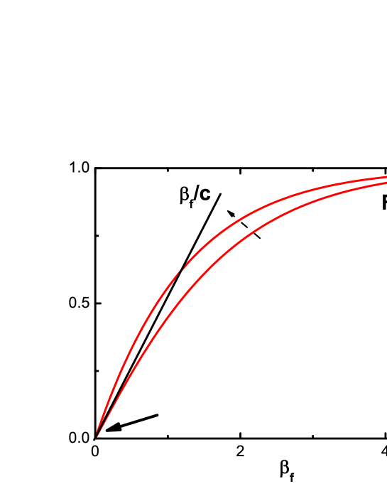
Figure 4: Increasing $f$ beyond the tricritical value of $1/2$, one observes that $\beta_{f}$ changes smoothly. Here, the dotted arrow denotes an increase in $f$.

II.2.2 $f<1/2$

When $f<1/2$, Figure 1 gives us an indication of the scaling behavior near the transition. By increasing the slope of the straight line, i.e. decreasing $c$, the first solution, $\beta_{f}=\beta_{0}>0$, appears when the line is tangent to $F(\beta_{f})$ such that the critical average connectivity is

$$\frac{1}{c_{G}}=e^{-\beta_{0}}[(1-f)\beta_{0}+f].$$ (29)

Increasing $c_{G}$ by $\epsilon$ and assuming$\beta_{f}=\beta_{0}+A\epsilon^{\lambda}$, where $A$ and $\lambda$ are positive constants, and then the LHS of Eq. 23 becomes

$$\frac{\beta_{0}+A\epsilon^{\lambda}}{c_{G}+\epsilon}=\frac{1}{c_{G}}(\beta_{0}+A\epsilon^{\lambda})(1-\frac{\epsilon}{c_{G}})=\frac{1}{c_{G}}(\beta_{0}-\frac{\beta_{0}}{c_{G}}\epsilon+A\epsilon^{\lambda}-\frac{A}{c_{G}}\epsilon^{\lambda+1}),$$ (30)

and the RHS becomes

$$1-e^{-\beta_{0}-A\epsilon^{\lambda}}[1+(1-f)(\beta_{0}+A\epsilon^{\lambda})]$$ (31)

$$= 1-e^{-\beta_{0}}(1-A\epsilon^{\lambda}+\frac{1}{2}A^{2}\epsilon^{2\lambda}-\frac{1}{6}A^{3}\epsilon^{3\lambda}+\mathcal{O}(\epsilon^{3\lambda}))[1+(1-f)(\beta_{0}+A\epsilon^{\lambda})].$$

According to Eq. 30 and Eq. 31, the constant terms and the $\epsilon^{\lambda}$ terms on both sides cancel each other, thus, the lowest order of the RHS, i.e. $\epsilon^{2\lambda}$, should cancel the $\epsilon$ term on the LHS leading to $\lambda=1/2$. To find the scaling of the size of the giant component with the initial average connectivity, $1-t_{f}\propto\beta_{f}\propto B+C\epsilon^{1/2}$, where $B$ and $C$ are positive constants. In other words, the transition is discontinuous.

II.2.3 $f>1/2$

Figure 2 qualitatively demonstrates that the onset of a nonzero $\beta_{f}$ as a function of $c$ is a continuous transition starting at $\beta_{f}=0$. The critical value of $c$ is given by

$$f=\frac{1}{c_{G}}.$$ (32)

As $c$ is increased by $\epsilon$ to $c_{G}+\epsilon$ and assuming $\beta_{f}$ changes continuously from zero, $\beta_{f}\sim\epsilon$. Therefore,

$$1-t_{f}\sim\epsilon^{2}$$ (33)

near the transition. This scaling is to be contrasted with the scaling at the tricritical point where the order parameter exponent is unity.

One can also investigate the scaling of the transition with $f$. As $f$ changes from $f_{0}$ to $f_{0}+\epsilon$, $\beta_{f}$ changes from $0$ to $A\epsilon^{\lambda}$. Then, the LHS of Eq. 23 becomes

$$\frac{A\epsilon^{\lambda}}{c},$$ (34)

and the RHS becomes

$$1-(1-A\epsilon^{\lambda}+\frac{1}{2}A^{2}\epsilon^{2\lambda}-\frac{1}{6}A^{3}\epsilon^{3\lambda}+\mathcal{O}(\epsilon^{3\lambda}))+(f_{0}-1+\epsilon)(1-A\epsilon^{\lambda}+\frac{1}{2}A^{2}\epsilon^{2\lambda}-\frac{1}{6}A^{3}\epsilon^{3\lambda}+\mathcal{O}(\epsilon^{\lambda}))A\epsilon^{\lambda}$$ (35)

with

constant term $$= 0;$$

$${\epsilon}^{\lambda}\textrm{ term} = f_{0}A\epsilon^{\lambda};$$

$${\epsilon}^{2\lambda}\textrm{ term} = (\frac{1}{2}-f_{0})A^{2}\epsilon^{2\lambda};$$

$${\epsilon}^{\lambda+1}\textrm{ term} = A\epsilon^{\lambda+1};$$

$${\epsilon}^{3\lambda}\textrm{ term} = (\frac{f_{0}}{2}-\frac{1}{3})A^{3}\epsilon^{3\lambda}.$$

The $\epsilon^{\lambda}$ terms cancel each other on both sides and $\epsilon^{\lambda+1}$ and $\epsilon^{2\lambda}$ terms sum to zero leading to $\lambda=1$ and $A=\frac{1}{f_{0}-\frac{1}{2}}$. Thus, the scaling of $1-t_{f}$ with a small change in $f$ is the same as for a small change in $c$. We see that the amplitude diverges when $f_{0}=1/2$ indicating the vanishing of the $\beta_{f}^{2}$ contribution such that the cubic contribution comes into play when $f=1/2$.

II.2.4 Summary

Our results for the hybrid $k_{1}=2$ and $k_{2}=3$-core on the random graph can be summarized in the phase diagram depicted in Figure 5. For $f>1/2$, the $k_{1}=2$-core dominates and the transition is continuous with the size of the giant component scaling quadratically with a small increase in the initial average connectivity beyond its critical value. For $f=1/2$ there exists a tricritical point with a new order parameter exponent, and for $f<1/2$ the transition is discontinuous.

Figure 5: The $c,f$ phase diagram. To the left of the boundary there is no giant component and to the right there is.

III Hybrid $k$-core and jamming percolation models in two dimensions

In order to understand what happens in the hybrid models, we first review two jamming percolation models since they are rather new to the field. These models are vertex models (no edges are explicitly added). Of course, a pure vertex version of $k$-core percolation can also be introduced where an occupied vertex requires at least $k$ occupied vertices to remain occupied. It is this version of $k$-core we will refer to in the following section.

III.1 Counter-balance model

While $k\geq 3$-core exhibits a discontinuous transition in mean-field, there is no known two-dimensional example of $k\geq 3$-core exhibiting a discontinuous transition. In fact, it appears that $k\geq 3$-core on two-dimensional lattices either exhibits an ordinary percolation transition with a shift in the critical occupation probability, or there is no transition until the lattice is fully occupied triangular lattice ; pc=1 . For instance, simulations of $k=3$-core percolation on the triangular lattice result in similar ordinary percolation exponents, while for $4\geq k\geq 6$, $p_{c}=1$. A heuristic argument behind the former result is that finite clusters are allowed for $k=3$ with a fully occupied hexagon being the smallest structure. One can then imagine this object to be smallest object, as opposed to a single vertex, such that path-like spanning structures are formed out of fully occupied hexagons. This procedure is a simple coarse-graining on a microscopic scale and will not effect the macroscopic scales near a continuous phase transition.

Inspired by the jamming transition in two-dimensions where the fraction of particles participating in the jammed structure goes from zero to finite jamming1 ; jamming2 , one can encode various properties of the jammed packings into a percolation model. One of those properties is counter-balancing. For the force on each particle to be balanced, there must be an occupied particle on either side. Of course, in two-dimensions, two particles on opposite sides of the particle in question will not suffice since the configuration is not mechanically stable. However, three particles whose centers are 120 degrees with respect to each other as measured from the center particle is a stable configuration.

Counter-balance percolation takes into account the counter-balancing aspect of force-balance cb . As for an example, we begin with a two-dimensional square lattice. Each vertex neighbors all vertices within a 5x5 square modulo itself. In other words, each vertex has 24 nearest neighbors. The counter-balancing constraint is the following: for an initially occupied vertex to remain occupied, there must be at least one occupied neighbor in set A, which in turn calls for at least one occupied neighbor in set B, and there must be at least one occupied neighbor in set C, which in turn calls for at least one occupied neighbor in set D. The four sets A, B, C, and D, are defined in Fig. 6. The counter-balance constraint can be succinctly stated as: (A and B) and (C and D), where each letter X is short for “at least one occupied vertex in set X”. Note that the counter-balance constraint is defined in such a way such that vertical and/or horizontal lines of occupied vertices are, by themselves, not stable. Fig. 7a demonstrates an allowed configuration and Fig. 7b demonstrates a forbidden configuration.

To enforce the counter-balance constraint, we initially occupy vertices on the lattice with independent occupation probabilities $p$, and then repeatedly remove occupied vertices that violate the counter-balance constraint, until all remaining occupied vertices obey the constraint. Note that $p$ is the occupation density before culling, and generically differs from the final occupation density. Moreover, the model is abelian, i.e. the order of the culling does not affect the final configuration.

Figure 6: Force-balance model on the 2$d$ square lattice with 24 nearest neighbors.

Figure 7: Black sites denote occupied sites, and red sites denote unoccupied sites. (a) Allowed configuration. (b) Forbidden configuration. While the number of occupied nearest neighbors is greater than three, the force-balance condition is violated.

Numerical simulations of the counter-balance model strongly suggest a discontinuous transition with a finite fraction of vertices participating in the spanning cluster at the transition cb . Of course, numerical simulations can be misleading as has been demonstrated in the past, and so one looks for evidence beyond numerics. Such evidence is provided for by studying a simpler, but related, jamming percolation model, namely the spiral model. While the spiral model is less physical, one can make several concrete statements about its percolation transition.

III.2 Spiral model

The spiral model spiralmodel2 is defined as the following. Again, we begin with a square lattice. The neighbors of each vertex contain the four nearest neighbors and the four next nearest neighbors to make a total of eight neighbors. After the initial random occupation of vertices, for each vertex to remain occupied there must be at least one occupied neighbor in set A and at least one occupied neighbor in B, or there must be at least one occupied neighbor in set C and one occupied neighbor in set D. See Fig. 8 to denote the sets.

It turns out that the critical occupation probability for this model is the same as for directed percolation dp , denoted as $p_{c}^{DP}$. One can see the link with directed percolation when considering only sets A and B or sets C and D. Each pair of sets is isomorphic to the canonical two-dimensional version of directed percolation with two neighbors above and below each vertex. Therefore, for $p>p_{c}^{DP}$, there exists a spanning cluster along either diagonal. Since there are two pairs of sets one might argue that the critical occupation probability is lower than that of directed percolation. However, one can show that a certain class of voids (finite “clusters” of unoccupied vertices) cause all remaining occupied vertices in the system to become unoccupied as long as $p<p_{c}^{DP}$. Given the two bounds, $p_{c}^{SP}=p_{c}^{DP}$, where $SP$ denotes the spiral model.

Figure 8: The sets in the spiral model.

While determining $p_{c}^{SP}$ is a detail, it is an important one for arguing that the percolation transition is discontinuous, which is very different from the continuous transition in directed percolation. To argue for a discontinuity, one can construct a set of spanning structures, which include the origin, and demonstrate that for $p=p_{c}^{DP}$, the probability of such a set is greater than zero. In other words, the spanning structure is compact at the transition. This argument involves the notion of T-junctions, which characterize one diagonal path being supported by the other diagonal path. For instance, a nonspanning path along one diagonal can survive only if it is sandwiched between two paths of the other diagonal. See Figure 9.

Figure 9: A pair of T-junctions in the spiral model.

To observe compact spanning structures at the transition, one can build a spanning structure beginning with a rectangle whose long side is along the A-B diagonal and includes the origin. Then, one considers an infinite sequence of pairs of rectangles of increasing size emanating outward from the initial rectangle and intersecting as indicated in Figure 10. If each of the A-B rectangles contains an A- B spanning path along its length, it is indeed a spanning structure containing the origin due to the existence of T-junctions. From what is known about directed percolation at the transition, one can show that the probability for each of the A-B rectangles to contain a A-B spanning path is indeed greater than zero such that this compact spanning structure exists at the transition. Please see Ref. spiralmodel2 for details.

It turns out that one can extend these arguments to jamming percolation models with more than two pairs of sets momo&jen . However, these arguments have not yet been extended to sets with more than two sites. The universality of directed percolation should allow for such an extension since as long as the sets are arranged in opposite pairs, the occupation for each pair of sets is governed by a directed percolation-type process. It turns out that the rules for the counter-balance model can be written as a spiral-like model with more than two pairs of sets with some sets containing more than two vertices. See Figure 11. In addition, the conversion also involves triplets and quadruplets of sets (as opposed to just pairs) with each set participates in, for example, a pair-wise interaction as well as a three-way interaction. These triplets and quadruplets of sets have not yet been addressed in the context of a spiral-type model but should not invalidate the overall construction of the above argument. The fact that one set participates in several interactions increases the possible configurations, but, again, should not invalidate the above argument. Therefore, we expect the percolation transition in the counter-balance model to be discontinuous with numerical evidence supporting this expectation cb .

Figure 10: Schematic of a spanning structure in the spiral model where a path spans each rectangle.

Figure 11: The counter-balance rules can be implemented with (A’ and C’) or (D’ and B’) or (E’ and B’ and C’) or (F’ and C’ and D’) or (G’ and A’ and B’) or (H’ and A’ and D’) or (A’ and G’ and H’) or (B’ and E’ and G’) or (C’ and E’ and F’) or (D’ and F’ and H’) or (E’ and F’ and G’ and H’).

III.3 Tricriticality in the hybrid $k$-core/spiral model?

For the spiral model, the notion of a T-junction as well as properties of directed percolation are key in establishing a discontinuous transition. What happens when the model is perturbed by having an infinitesimal fraction of vertices with the $k$-core condition replacing the spiral condition? To answer this question, we must first choose $k$. The value of $k$ is chosen such that $p_{c}$ for the lattice with every vertex obeying the $k$-core condition is less than $p_{c}^{DP}$. For example, $k=3$ satisfies this condition. Note that each vertex has the same eight neighbors as in the spiral model. In addition, when all vertices are $k$-core vertices, we assume that the transition is continuous and in the same universality class as ordinary percolation. This model is similar to the $k=3$-core transition on the triangular lattice. In both cases, there exist small clusters that survive the culling process such that, heuristically, these clusters link up to form path-like structures as occurs in ordinary percolation.

Given the properties of the all $k$-core transition, as the fraction of spiral model vertices increases from zero, the critical occupation probability increases since the $k$-core condition is less constraining than the spiral model condition. As long as the critical occupation probability is less than $p_{c}^{DP}$, the construction invoking a spanning scaffold of T-junctions at $p_{c}^{DP}$ to demonstrate a discontinuous transition for the all spiral model vertices no longer holds. The integrity of the T-junctions to arrive a spanning structure is destroyed with finite clusters now allowed even for an infinitesimal fraction of $k$-core vertices. T-junctions are no longer necessary to support a structure. This property is consistent with the violation of the former bound, $p>p_{c}^{DP}$, since each diagonal is no longer isomorphic to directed percolation independently. The second former bound, $p<p_{c}^{DP}$, also breaks down since the growth of voids is now stopped by $k$-core vertices.

The existence of finite clusters for any fraction of $k$-core vertices is certainly different from the spiral model where no finite clusters are allowed. Does the existence of finite clusters imply that the transition is continuous up until all $k$-core vertices are replaced with spiral model ones? In fact, there’s no direct relationship between the existence of finite clusters and the continuity of a transition. One can construct a model occupying vertices at random and independently and then remove all finite clusters. While this particular constraint is highly non-local, it preserves the properties of the spanning cluster (of ordinary percolation) at the transition. Even so, we argue that the transition is continuous for the following reason. As the fraction of spiral model vertices increases, their increasing presence demands the increasing use of T-junctions to support spiral model vertices where two paths along one diagonal sandwich and support the path along the second diagonal. However, these two supporting paths can now end on $k$-core sites as opposed to other T-junctions to form finite clusters. Two finite clusters whose interiors each contain spiral model sites can join in such a way that the removal of one site in the two cluster formation that is not shared by both clusters before the joining does not induce the removal of the other cluster. We speculate that this independent cluster joining property leads to a continuous transition since the joining of such clusters leads to path-like structures on a larger scale as clusters are placed “side-by-side”. The larger the clusters, the larger the scale one has to go to “observe” the path-like structures. See Figure 12.

One would like to make the speculation that the independent cluster joining property leads to a continuous transition more rigorous. Such speculation may lead to a framework to prove that the transition for similar models, such as $k=3$-core on the triangular lattice, is in the same universality class as ordinary percolation. Currently, there is only numerical evidence for $k=3$-core on the triangular lattice being in the same universality class as ordinary percolation.

Figure 12: An example of two finite clusters for $k=3$-core in the eight neighbor model sharing a boxed occupied vertex. The removal of any occupied vertex to the right of the boxed occupied vertex does not trigger the removal of any occupied vertex to the left of the boxed occupied vertex.

So, even for an infinitesimal fraction of $k$-core vertices with all other vertices dictated by the spiral model, we speculate that the transition is in the same universality class as ordinary percolation. In other words, only when all vertices are spiral model vertices is there a discontinuous transition. Given this scenario, we speculate that there is no tricritical point in this hybrid of $k=3$-core and the spiral model.

III.4 Tricriticality in hybrid $k$-core/counter-balance model?

Since the counter-balance model can be expressed as spiral model-type constraints, what happens in the hybrid $k$-core/spiral model may resemble what happens in the hybrid $k$-core/counter-balance model. Therefore, we expect that the transition is continuous as long as $1-f=g<1$, where $g$ is the fraction of counter-balance vertices, with $k=3$. We now provide numerical evidence to support this claim.

First, in Figure 13 we plot the differential curve for the probability of spanning, $P_{span}$, as a function of $p$ for $g=0$ and $k=3$ with 24 nearest neighbors on the square lattice. The system length is denoted by $L$ and periodic boundary conditions are implemented. The position of the peak denotes the critical occupation probability, $p_{c}$, for each particular system size. We then perform a scaling collapse using the correlation length exponent of ordinary percolation $\nu=4/3$. See the inset to Figure 13. The scaling collapse is reasonable suggesting that the transition is at least consistent with the ordinary percolation universality class as should be the case for $g<1$ given the discussion in the previous subsection.

Figure 13: Differential for the probability of spanning, $P_{span}$, as a function of occupation probability $p$ for $g=0$. Different system sizes are studied. The inset demonstrates the finite-size scaling for $P_{span}(p)$ using the correlation length exponent for ordinary percolation.

Next, we plot average size of any spanning cluster, $<S>$ (the brackets denote the configuration averaging) as a function of the initial occupation probability $p$ for different $g$s. See Fig. 14. In an infinite system, for $g<1$, we expect $<S>=A(g)(p-p_{c}(g))^{5/36}$ for $p>p_{c}(g)$ and zero otherwise. In a finite system, this function will be smoothed out. As expected, we observe that $p_{c}(g)$ increases with increasing $g$. The curves, even for $g=1$, appear to be sharpening with increasing $g$ as well such that the amplitude $A(g)$ increases with increasing $g$. However, the $<S>$ versus $p$ curves appear qualitatively similar, so how does one differeniate between a continuous transition and a discontinuous one?

We can do so by examining the distribution of the sizes of the spanning cluster as opposed to just looking at the average size. See Figs. 15 and 16. To compare distributions among the different $g$s, we plot the distribution for the same average spanning size, which means $p$ changes from curve to curve. The distribution for $g=0$ has a well-defined peak at small values of $S$, small meaning much less than unity. As $g$ increases from zero, the distribution for $S$ looks similar with a slight shift in the distribution. It is not until $g\approx$ 0.99 that the position of peak increases such that it is much greater than the fixed average size of 0.05 indicating that in many instances no spanning cluster found and when they are found, the spanning cluster is much larger than the average. This feature of the distribution, as long as it persists in the infinite system limit, is characteristic of a discontinuous percolation transition. When the system size is increased for fixed $g$, we observe that the position of the peak shifts to the left indicating that the transition becomes more continuous even for $g=0.99$. Therefore, the numerical data supports our scenario of the absence of a discontinuous transition until $g=1$ and no tricritical point.

Figure 14: Average size of spanning cluster, $<S>$, as a function of $p$ for a mixture of $k=3$-core and counter-balance percolation vertices. For $g=0$, the vertices are all $k$-core. For $g=1$, the vertices are all counter-balance. Even for $g=0.96$, the curve resembles the $g=0$ (continuous) case. Here, the system length, $L$, is $L=256$.

Figure 15: Distribution of the size of spanning cluster, $S$, for different $g$s. For $g=1$, the vertices are all counter-balance. Only for $g=0.99$ does the distribution begins to shift to the right significantly, whereas for $g=0.98$ the distribution more closely resembles the $g=0$ case. Here, again, $L=256$. The no spanning cluster contributions are not shown.

Figure 16: Distribution of the size of spanning cluster, $S$, for different $g$s and for different system lengths. Note that as $L$ increases, the curves for $g=0.99$ shift to the left indicating that as $L$ becomes large, the transition approaches the $g=0$ continuous case as opposed to the $g=1$ discontinuous case.

IV Discussion

There has been a recent proliferation of percolation models going beyond the original model, where edges/vertices are randomly and independently added to a network, to find discontinuous transitions. While much of this proliferation is driven by what is called explosive percolation, there has been, shall we say, quieter progress on what is called jamming percolation models inspired by jamming and glassy systems. Interestingly, there exists at least one example of a discontinuous percolation transition on random graphs, called $k$-core percolation, which was posed back in 1979 CLR ; Wormald3authors . However, this transition is not the ordinary type of discontinuous transition lacking any diverging lengthscales. In fact, the $k\geq 3$-core transition exhibits several diverging lengthscales. In addition, the spiral model, and its related counter-balance model, provide examples of discontinuous percolation transitions in two-dimensions, again, with diverging lengthscales spiralmodel2 ; cb .

Since both $k\geq 3$-core and the spiral model exhibit discontinuous transitions, it may be useful to investigate what properties they share in order to execute a more efficient search for other discontinuous percolation transitions. Both models share the property of not “allowing” finite clusters. In the spiral model, this property is exact. For the $k$-core model on trees, this property is exact. On random graphs, this property is approximate but becomes an increasingly better approximation in the thermodynamic limit. One may argue that forbidding finite clusters implies a discontinuous transition, at least in low-dimensions. However, this is not the case, since one can construct the usual percolation model on the square lattice and remove any finite clusters using a non-local rule. One can also do this using a local rule using only one pair of sets from the spiral model.

The nontrivial nesting of the spanning structure in the spiral model with the two diagonals interdependent on one another tells us that even if finite clusters are allowed, the formation and subsequent joining of even finite clusters should be non-local in the sense the removal of one vertex in a cluster signals the removal of at least a finite fraction of vertices in its formerly disjoint neighboring clusters. The rarefication rarefication of the lattice or a cluster aggregation model with a non-local kernel clusteraggregation ; clusteraggregation2 provide such mechanisms for nontrivial cluster joining such that the transition is discontinuous. On the flip side, we speculate that perhaps the independent finite cluster joining property, where the removal of one vertex in one of the two finite clusters (determined prior to joining) that is not shared by the other does not induce the removal of the other finite cluster. This property provides for a simple path-like joining of finite clusters such that an ordinary percolation transition presumably occurs as is found in $k\geq 3$-core models in finite dimensions.

Given the existence of both continuous and discontinuous percolation transitions, one may form hybrid models of the two types to search for a tricritical point separating the continuous regime from the discontinuous regime. Using a mixture of $k=2$-core and $k=3$-core vertices on random graphs, we find a tricritical point and determine the size of the giant component as a function of the average connectivity. While two previous works have identified this point Cellai ; Branco , we use a different dynamical method via a rate equation approach, which could prove to be valuable for investigating other correlated percolation models as the constraints become complex. Of course, our results using the rate equation approach agree with previous results using a “static” method.

Moreover, we investigate the possibility of a tricritical point in two-dimensions. We do so with a mixture of $k=3$-core vertices and counter-balance vertices where the full $k=3$-core model exhibits a continuous transition (which differs from mean-field) and the full counter-balance model exhibits a discontinuous phase transition. We argue that there is no tricritical point in this mixed model since the discontinuous transition occurs only in the full counter-balance model. However, we expect interesting crossover behavior between to the two types of transitions that should be explored. This result is the first we know of with a line of continuous transitions ending at a discontinuous transition, which is to be compared with the water phase diagram where there is a line of discontinuous transitions ending at a continuous one. In addition, this result is to be contrasted with the work of Cellai and collaborators studying a mixture of $k=2$ and $k=3$-core vertices on the square lattice Cellai . For the full $k=2$-core model on the square lattice, the transition is continuous, while for the full $k=3$-core model, $p_{c}=1$ with interesting crossover behavior between the two cases. This result is also to be contrasted with the tricriticality obtained in a diluted $Q$-state Potts model on a triangular lattice tricriticalPotts .

Finally, what about ties between mixed correlated percolation models and physical systems? The introduction of hetereogeneities into the Frederickson-Anderson model for glassy systems maps to the mixed $k$-core model Sellitto . Moreover, there is a recent experiment jammingbyshear where a two-dimensional packing of frictional disks is sheared at a packing fraction just below the shear-free jamming transition to induce jamming. At small applied shear stress, a subset of the contact network of the jammed states exhibits spanning structures along one direction only, while at larger applied shear stress, the spanning structures (of a subset of the contact network) percolate in both directions. One can perhaps model the connectivity of the spanning structures as the applied shear stress is varied by taking a mixture of the usual counter-balance model and an anisotropic version of the counter-balance model where only sets A and B are considered. More specifically, as the applied shear stress is increased the ratio of counter-balance vertices to anisotropic counter-balance vertices increases. However, since only a subset of the contact network is used in obtaining this result, some finite structures may be allowed.

JMS acknowledges support from NSF-DMR-CAREER Award 0645373.

References

- (1) S. Broadbent and J. Hammersley, “Percolation processes I. Crystals and mazes”, Proc. Cam. Phil. Soc. 53, 629 (1957).
- (2) D. Stauffer and A. Aharony, Introduction to percolation theory (London: Taylor and Francis, 1994).
- (3) B. Bollobas and O. Riordan, Percolation (London: Cambridge University Press, 2006).
- (4) D. Achlioptas, R. M. D’Souza, and J. Spencer, “Explosive percolation in random networks”, Science, 323, 1453 (2009).
- (5) H. J. Herrmann and N. A. M. Araujo, “Watersheds and Explosive percolation”, Physics Procedia, 15, 37 (2011).
- (6) E. J. Friedman and A. S. Landsberg, “Construction and analysis of random networks with explosive percolation” Phys. Rev. Lett. 103, 255701 (2009).
- (7) R. M. D’Souza and M. Mitzenmacher, “Local cluster aggregation models of explosive percolation”, Phys. Rev. Lett., 104, 195702 (2010).
- (8) F. Radicchi and S. Fortunato, “Explosive percolation:a numerical analysis”, Phys. Rev. E 81, 036110 (2010).
- (9) O. Riordan and L. Warnke, “Explosive Percolation Is Continuous”, Science, 333, 322 (2011).
- (10) R. A. de Costa, S. N. Dorogovtsev, A. V. Goltsev, and J. F. F. Mendes, “Explosive percolation is actually continuous”, Phys. Rev. Lett. 105, 255701 (2010).
- (11) R. M. Ziff, “Explosive growth in biased dynamic percolation on two-dimensional regular lattice networks”, Phys. Rev. Lett., 103, 045701 (2009).
- (12) R. M. Ziff, “Scaling behavior of explosive percolation on the square lattice”, Phys. Rev. E, 82, 051105 (2010).
- (13) T. Bohman, A. Frieze, and N. C. Wormald, “Avoidance of a giant component in half the edge set of a random graph”, Random Struct. Algorithms, 25, 432 (2004).
- (14) W. Chen and R. M. D’Souza, “Explosive percolation with multiple giant components”, Physica A, 106, 115701 (2011).
- (15) W. Chen and R. M. D’Souza, “Slow convergence tunes onset of strongly discontinuous explosive percolation”, arXiv:1106.2088v2 (2011).
- (16) K. J. Schrenk, A. Felder, S. Deflorin, N. A. M. Araujo,R. M. D’Souza, and H. J. Herrmann, “Bohman-Frieze-Wormald model on the lattice, yielding a discontinuous percolation transition”, Phys. Rev. E 85, 031103 (2012).
- (17) J. Chalupa, P. L. Leath, and G. R. Reich, “Bootstrap percolation on a Bethe lattice”, J. Phys. C: Solid State Phys. 12, L31 (1979).
- (18) S. N. Dorogovtsev, A. V. Goltsev, and J. F. F. Mendes, “-core organization of complex networks”, Phys. Rev. Lett. 96, 040601 (2006).
- (19) J. M. Schwarz, A. J. Liu, and L. Q. Chayes, “The onset of jamming as the sudden emergence of an infinite k-core cluster,” Europhys. Lett. 73, 560 (2006).
- (20) M. C. Medeiros and C. M. Chaves, “Universality in bootstrap and diffusion percolation”, Physica A, 234, 604 (1997).
- (21) M. Aizenmann and J. Lebowitz, “Metastability effects in bootstrap percolation”, J. Phys. A 21, 3801 (1988).
- (22) P. De Gregorio, A. Lawlor, P. Bradley, and K. A. Dawson, “Exact solution of a jamming transition: Closed equation for a bootstrap percolation problem”, Proc, Natl. Acad. Sci. U S A 102, 5669 (2005).
- (23) A. B. Harris and J. M. Schwarz, “ expansion for -core percolation”, Phys. Rev. E 72, 046123 (2005).
- (24) C. Toninelli, G. Biroli and D. S. Fisher, “Jamming Percolation and Glass Transitions in Lattice Models”, Phys. Rev. Lett. 96, 035702 (2006).
- (25) M. Jeng and J. M. Schwarz, “Comment on “Jamming Percolation and Glass Transitions in Lattice Models.””, Phys. Rev. Lett. 98, 129601 (2007).
- (26) C. Toninelli1, G. Biroli, and D. S. Fisher, “Toninelli, Biroli, and Fisher Reply”, Phys. Rev. Lett. 98, 129602 (2007).
- (27) C. Toninelli and G. Biroli, “A New Class of Cellular Automata with a Discontinuous Glass Transition”, J. Stat. Phys. 130, 83 (2008).
- (28) N. A. M. Araujo, J. S. Andrade, Jr, R. M. Ziff and H. J. Herrmann, “Tricritical point in explosive percolation”, Phys. Rev. Lett. 106, 095703 (2011).
- (29) D, Cellai, A. Lawlor, K. A. Dawson, and J. P. Gleeson, “Tricritical Point in Heterogeneous k-Core Percolation,” Phys. Rev. Lett. 107, 175703 (2011).
- (30) R. K. Pan, M. Kivela, J. Saramake, K. Kaski, and J. Kertesz, “Explosive percolation on real-world networks”, arXiv:1010.3171.
- (31) H. D. Rozenfeld, L. K. Gallos, H. A. Makse, “Explosive percolation in human protein homology network”, Eur. Phys. J. B 75, 305 (2010). x
- (32) G. H. Fredrickson and H. C. Andersen, “Kinetic Ising Model of the Glass Transition”, Phys. Rev. Lett. 53, 1244 (1984).
- (33) E. R. Weeks, J. C. Crocker, A. C. Levitt, A. Schofield, and D. A. Weitz, “Three-dimensional direct imaging of structural relaxation near the colloidal glass transition”, Science, 287, 627 (2000).
- (34) M. Sellitto, G. Biroli, and C. Toninelli, “Facilitated spin models on Bethe lattice: Bootstrap percolation, mode-coupling transition and glassy dynamics”, Europhys. Lett. 69, 496 (2005).
- (35) M. Sellitto, D. De Martino, F. Caccioli, and J. J. Arenzon, “Dynamic Facilitation Picture of a Higher-Order Glass Singularity,” Phys. Rev. Lett. 105, 265704 (2010).
- (36) B. Pittel, J. Spencer, and N. C. Wormald, “Sudden Emergence of a Giant k-Core in a Random Graph,” J. Comb. Theory B 67, 111 (1996).
- (37) N. C. Wormald, Ann. Appl. Prob. “Differential Equations for Random Processes and Random Graphs”, 5, 1217 (1995).
- (38) A. K. Hartmann and M. Weigt, Phase Transitions in Combinatorial Optimization Problems, (Berlin: Wiley-VCH, 2005).
- (39) A. J. Liu and S. R. Nagel, “Jamming is just not cool any more”, Nature 396, 21 (1998).
- (40) C. S. O’Hern, L. Silbert, A. J. Liu, and S. R. Nagel, “Jamming at zero temperature and zero applied stress: the epitome of disorder”, Phys. Rev. E 68, 011306 (2003).
- (41) M. Jeng and J. M. Schwarz, “Force-balance percolation”, Phys. Rev. E 81, 011134 (2010).
- (42) H. Hinrichsen, “Nonequilibrium critical phenomena and phase-transitions into absorbing states”, Adv. Phys. 49, 815 (2000).
- (43) M. Jeng and J. M. Schwarz, “On the study of Jamming Percolation,” J. Stat. Phys. 131, 575 (2008).
- (44) S. Boettcher, V. Singh, and R. M. Ziff, “Ordinary percolation with discontinuous transitions,” Nat. Commun. 3 787 (2011).
- (45) Y.S. Cho, B. Kahng and D. Kim, “Cluster aggregation model for discontinuous percolation transition”, Phys. Rev. E 81, 030103 (2010).
- (46) S. S. Manna and A. Chatterjee, “A new route to explosive percolation”, Physica A, 390, 177 (2010).
- (47) N. S. Branco, “Probabilistic bootstrap percolation”, J. Stat. Phys. 70, 1035 (1993).
- (48) B. Nienhuis, A. N. Berker, Eberhard K. Riedel, and M. Schick, “First- and Second-Order Phase Transitions in Potts Models: Renormalization-Group Solution”, Phys. Rev. Lett. 43, 737 (1979).
- (49) D. Bi, J. Zhang, B. Chakraborty, and R. P. Behringer, “Jamming by shear”, Nature 480, 355 (2011).