Chandrasekhar theory of electromagnetic scattering from strongly conducting ellipsoidal targets

Abstract

Exactly soluble models in the theory of electromagnetic propagation and scattering are essentially restricted to horizontally stratified or spherically symmetric geometries, with results also available for certain waveguide geometries. However, there are a number of new problems in remote sensing and classification of buried compact metallic targets that require a wider class of solutions that, if not exact, at least support rapid numerical evaluation. Here, the exact Chandrasekhar theory of the electrostatics of heterogeneously charged ellipsoids is used to develop a “mean field” perturbation theory of low frequency electrodynamics of highly conducting ellipsoidal targets, in insulating or weakly conducting backgrounds. The theory is based formally on an expansion in the parameter $\eta_{s}=L_{s}/\delta_{s}(\omega)$, where $L_{s}$ is the characteristic linear size of the scatterer and $\delta_{s}(\omega)$ is the electromagnetic skin depth. The theory is then extended to a numerically efficient description of the intermediate-to-late-time dynamics following an excitation pulse. As verified via comparisons with experimental data taken using artificial spheroidal targets, when combined with a previously developed theory of the high frequency, early-time regime, these results serve to cover the entire dynamic range encountered in typical measurements.

I Introduction

There are a number of longstanding economic and humanitarian problems, such as clearance of unexploded ordnance (UXO) from old practice ranges, that require remote identification of buried metallic objects. The most difficult technological issue is not the detection of such targets, but rather the ability to distinguish between them and harmless clutter items, such as various sized pieces of exploded ordnance. Since clutter tends to exist at much higher density, even modest discrimination ability leads to huge reductions in the economic cost of remediating such sites.

I.1 Electromagnetic inverse problems

Formally, a successful solution to the electromagnetic (EM) discrimination problem is a theory or algorithm that allows derivation of accurate bounds on physical properties of the target scatterer (its position, shape, orientation, physical composition, etc.) from measurements of the scattered field using a well characterized experimental apparatus (with known transmitter and receiver coils, transmitted waveform, and so on). Solution of this inverse problem first requires the ability to generate high-fidelity candidate solutions to the forward problem, namely accurate computations of the scattered field from a known target in a known subsurface environment. The general solution to the forward problem requires full three dimensional numerical solutions to the Maxwell equations, a difficult and time consuming computational problem. To reduce the computational burden, it is extremely important to obtain analytic solutions to as broad an array of exactly soluble model problems as possible. These solutions may then either be used as crude models of the target, or as the basis of a perturbation scheme for accurate modeling of “nearby” target geometries.

The only compact targets for which a full analytic solution at any frequency may be derived are those with spherical symmetry Jackson . These are rather poor approximations to UXO, which tend to more resemble finite, rounded cylinders with roughly 4:1 aspect ratio. The approach pursued here is to take advantage of the fact that electrostatic solutions exist for a much broader array of target geometries, and that these solutions can then be used as the basis for a controlled perturbation theory, valid at low frequencies. The small parameter in the theory, $\eta_{s}\equiv L_{s}/\delta_{s}$, is the ratio of the electromagnetic skin depth $\delta_{s}(\omega)$ to the linear target size $L_{s}$. The theory is dubbed the “mean field approach,” since the smallness of $\eta_{s}$ means that the expansion is highly nonlocal in space, with the currents and fields at any given point in the target being sensitive to their values throughout the target. Although formally valid only for small $\eta_{s}$, we will see that the theory may be extended to higher frequencies, even where $\eta_{s}$ is significantly larger than unity, if one generates a sufficient number of terms in the series MITrefs .

The basic zeroth order theory requires one to solve for the electrostatic field generated by the target in a sequence of background fields of increasing complexity. The perturbation theory is developed formally for a general target shape, but even this sequence of simpler electrostatic problems generally requires a numerical solution. However, for the case of ellipsoids, such solutions may be computed analytically via an elegant approach developed by Chandrasekhar Chandra ; W2011 . Since many targets of interest may be modeled quite accurately by ellipsoidal or spheroidal shapes, the results of this paper have an immediately relevant application. The theory will mainly be illustrated for the case in which both background and scatterer are nonmagnetic (i.e., the permeability $\mu$ is a uniform constant), but the extension to permeable targets will be described as well.

When treating buried targets, the electrodynamics of the soil is also potentially important. We will assume that the ground is insulating or sufficiently weakly conducting that its response may be treated as quasistatic in the frequency range of interest (say, 100 kHz or less). Specifically, the background EM penetration depth (typically tens of meters or more at these frequencies) should be large compared to the measurement domain (typically on the scale of 1 m).

Even with the quasistatic assumption, the total electric field has a significant, unpredictable variability due to strong variation in the dielectric function due to varying soil type and inclusions, surface vegetation, air-ground interface, etc. It transpires, however, that an induction loop (EMI) measurement (as opposed, say, to a linear antenna measurement) is effectively sensitive only to the “magnetic part” (curl component) of the electric field, and that the latter is insensitive to the ground (partially explaining the ubiquity of such measurements in geophysics), so long as it is nonmagnetic foot:magsoils . In a happy confluence of theory and experiment, the perturbation theory is most efficiently formulated to isolate and compute precisely this part of the field.

I.2 Time-domain measurements

A common experimental probe for metallic targets is the time-domain electromagnetic (TDEM) measurement, in which one detects the inductive response of a target following termination of a transmitted pulse. The pulse generates a characteristic pattern of currents in the target, and the subsequent dynamics of, say, the electric field may be written as a superposition of EM eigenmodes:

$${\bf E}({\bf x},t)=\sum_{n=1}^{\infty}A_{n}{\bf e}^{(n)}({\bf x})e^{-\lambda_{n}t},$$ (1)

in which ${\bf e}^{(n)}$ is the mode shape, $\lambda_{n}$ the decay rate, and $A_{n}$ the excitation amplitude. This is analogous to the response of a drumhead following a strike. However, rather than corresponding to a set of characteristic eigenfrequencies (with, perhaps, some weak damping), the dissipative/ohmic dynamics leads here to modes that exhibit a pure exponential decay in time. The data will typically consist of the voltage measured in a receiver coil,

$$V(t)=\sum_{n=1}^{\infty}V_{n}e^{-\lambda_{n}t},$$ (2)

which is a superposition of the same exponential decays. The decay rates and mode shapes are, respectively, eigenvalues and eigenfunctions of the Maxwell equations at imaginary frequency $\omega_{n}=-i\lambda_{n}$, and may therefore be accessed through the perturbation technique developed here.

It transpires that in the high-contrast limit there are, in fact, two classes of excitation with widely separated decay rates. One set corresponds to electric polarization of the target, the primary example being an excitation in which a uniform electric field is suddenly switched off. These “electric modes” relax essentially instantaneously by direct equilibration of the charges induced on the target surface, and hence have very large, perturbatively inaccessible $\lambda_{n}$. On the other hand, the rapid relaxation implies that their contribution to the signal (2) disappears almost immediately.

The second, more interesting set of modes, corresponds to magnetic polarization of the target, the primary example being an excitation in which a uniform magnetic field is suddenly switched off. In this case circulating currents are generated. The flows are essentially tangential at the target boundary, produce no charge polarization, and therefore take much longer to relax. Being intrinsic to the geometry of the target, the current patterns associated with these “magnetic modes” must vary on the scale $L_{s}$ (or even on much smaller scales, as the decay rate increases and the mode shape becomes more spatially complex), and hence must lie in the regime $\eta_{s}(-i\lambda_{n})=O(1)$. Once again, however, these may be accessed via a sufficiently high-order expansion WL03 . Moreover, the exponential decay implies that as time progresses fewer and fewer of even these modes contribute to the signal, so that such a theory, which accurately computes only a finite set of the slowest decaying modes, would provide quantitative predictions on intermediate-to-late-time scales. On the other hand, in the opposite, early-time regime when a very large number of modes simultaneously contribute (but not so early that any electric modes still survive), a complementary “surface mode” theory, based on the diffusion of the initial screening current inward from the target surface, may be developed W2003 ; W2004 . It will be seen that these two regimes significantly overlap for a sufficiently high order mean field expansion, enabling a quantitative prediction of the signal over the full time-domain dynamic range.

I.3 Outline

The outline of the remainder of this paper is as follows. In Sec. II the basic content of the method is introduced, showing that it reduces to the evaluation of certain integrals of the Coulomb interaction over the volume of the scatterer. In Sec. III the Chandrasekhar theory of ellipsoidal electrostatics Chandra is reviewed, showing that it too reduces to this same class of integrals. In Sec. IV this connection is used to derive explicit expressions for the scattering integrals. In Secs. V and VI these are evaluated explicitly for the case of solid homogeneous ellipsoids. In Sec. VII the solution to the frequency-domain scattering problem in a known background field is obtained first formally, and then explicitly to $O(\eta_{s}^{2})$. Electric and magnetic excitations are identified, the latter being the low frequency precursors to the freely decaying magnetic modes. In Sec. VIII, the time-domain response is discussed. Successful comparisons of the theory, extended numerically to significantly higher order in $\eta_{s}$, to real data from artificial spheroidal targets are demonstrated.

Finally, in Sec. IX we conclude by describing generalizations of the theory (whose detailed applications will be left to future work). In Sec. IX.1 we consider permeable targets, $\mu\neq\mu_{b}$. In Sec. IX.2 we consider simplifications in the high contrast limit $\mu/\mu_{b}\gg 1$, relevant to ferrous targets where $\mu/\mu_{b}=O(10^{2})$. In Sec. IX.3 we consider the computation of the freely decaying modes for permeable targets. In Sec. IX.4 we consider more realistic target geometries, including hollow targets and multiple targets. Finally, in Sec. IX.5 we consider the effects of background permeability variations.

II Mean Field approach to low frequency, high contrast scattering

The mean field approach is based on the Green function formulation of electromagnetic scattering. Let $\epsilon_{b}({\bf x},\omega)$ and $\epsilon({\bf x},\omega)$ be the space- and frequency-dependent dielectric constant for background and background plus target, respectively. At low frequencies these take the form (in Gaussian units, which are used throughout unless explicitly stated otherwise),

$$\epsilon_{b}=\epsilon_{b}^{\prime}+\frac{4\pi i\sigma_{b}}{\omega},\ \ \ \ \epsilon=\epsilon^{\prime}+\frac{4\pi i\sigma}{\omega},$$ (3)

where $\epsilon_{b}^{\prime}({\bf x})$, $\epsilon^{\prime}({\bf x})$ are static dielectric constants and $\sigma_{b}({\bf x})$, $\sigma({\bf x})$ are DC conductivities. All four quantities are real and frequency independent. Let $k\equiv\omega/c$ be the vacuum wavenumber, and define

$$\kappa_{b}^{2}=\epsilon_{b}\mu_{b}k^{2},\ \ \kappa^{2}=\epsilon\mu k^{2},\ \ Q=\kappa^{2}-\kappa_{b}^{2}.$$ (4)

For most of this paper, it will be assumed that the permeability $\mu=\mu_{b}$ is a uniform constant, the same for both background and target. Generalization to inhomogeneous $\mu$ will be discussed in Sec. IX. In addition, at the low frequencies of interest, $\epsilon_{b}^{\prime},\epsilon$ are negligible compared to the conductivity contributions and will usually be dropped foot:ebprime . The high contrast assumption corresponds to $|\kappa^{2}/\kappa_{b}^{2}|=|\epsilon/\epsilon_{b}|\sim\sigma/\sigma_{b}\gg 1$. Typical metallic conductivities are in the range $\sigma\sim 10^{7}$ S/m, while typical ground conductivities are in the range $\sigma_{b}\sim 0.1$ S/m, so the ratio $\sigma/\sigma_{b}\sim 10^{8}$ is indeed extremely large.

II.1 Green function formulation

The background and full electric fields (with uniform $\mu$) satisfy the frequency domain wave equations

$$\nabla\times\nabla\times{\bf E}_{b}-\kappa_{b}^{2}{\bf E}_{b} = {\bf S}$$

$$\nabla\times\nabla\times{\bf E}-\kappa^{2}{\bf E} = {\bf S},$$ (5)

in which ${\bf S}({\bf x})=(4\pi i\mu k/c){\bf j}_{S}({\bf x})$ is proportional to the source current distribution ${\bf j}_{S}$. The latter is generated by a transmitter coil that is assumed to be external to the target region. The associated source charge distribution is $\rho_{S}=(i\omega)^{-1}\nabla\cdot{\bf j}_{S}$. The magnetic fields follow from the relation $ik{\bf B}=ik\mu{\bf H}=\nabla\times{\bf E}$.

Let ${\bf\hat{G}}({\bf x},{\bf x}^{\prime})$ be the $3\times 3$ tensor Green function for the background medium, satisfying,

$$\nabla\times\nabla\times{\bf\hat{G}}({\bf x},{\bf x}^{\prime})-\kappa_{b}({\bf x})^{2}{\bf\hat{G}}({\bf x},{\bf x}^{\prime})=\delta({\bf x}-{\bf x}^{\prime})\openone.$$ (6)

${\bf\hat{G}}$ is symmetric, but self adjoint only if $\kappa_{b}^{2}$ is real. For a uniform, homogeneous background medium one obtains the exact solution

$${\bf\hat{G}}({\bf x},{\bf x}^{\prime})=\left(\openone+\frac{1}{\kappa_{b}^{2}}\nabla\nabla\right)g({\bf x},{\bf x}^{\prime}),$$ (7)

with scalar Green function

$$g({\bf x},{\bf x}^{\prime})=\frac{e^{i\kappa_{b}|{\bf x}-{\bf x}^{\prime}|}}{4\pi|{\bf x}-{\bf x}^{\prime}|},$$ (8)

satisfying the Helmholtz equation, $-(\nabla^{2}+\kappa_{b}^{2})g=\delta({\bf x}-{\bf x}^{\prime})$. The background electric field may then be expressed in the form

$${\bf E}_{b}({\bf x})=\int d^{3}x^{\prime}{\bf\hat{G}}({\bf x},{\bf x}^{\prime})\cdot{\bf S}({\bf x}^{\prime}),$$ (9)

The operator acting on $g$ in (7) essentially enforces transverse polarization via the divergence condition $\nabla\cdot(\epsilon_{b}{\bf E}_{b})=4\pi\rho_{S}$. Note that quite generally, as indicated by (7) and (8), ${\bf\hat{G}}$ has a $|{\bf x}-{\bf x}^{\prime}|^{-3}$ divergence at small separation, hence there is a potential logarithmic singularity in (9). The integral over the anisotropic dipole-like angular dependence regularizes this singularity, but careful limiting procedures must still be used when dealing with Green function integrals of this type.

By taking the difference of the two lines of (5), the source ${\bf S}$ drops out and one obtains

$$\nabla\times\nabla\times({\bf E}-{\bf E}_{b})-\kappa_{b}^{2}({\bf E}-{\bf E}_{b})=Q{\bf E}.$$ (10)

Applying the Green function to both sides, the full field satisfies the integral equation,

$${\bf E}({\bf x}) = {\bf E}_{b}({\bf x})+\int_{V_{s}}d^{3}x^{\prime}Q({\bf x}^{\prime}){\bf\hat{G}}({\bf x},{\bf x}^{\prime})\cdot{\bf E}({\bf x}^{\prime})$$ (11)

$$= {\bf E}_{b}({\bf x})+\left(\openone+\frac{1}{\kappa_{b}^{2}}\nabla\nabla\right)\cdot\int_{V_{s}}d^{3}x^{\prime}g({\bf x},{\bf x}^{\prime})$$

$$\hskip 108.405pt\times\ Q({\bf x}^{\prime}){\bf E}({\bf x}^{\prime}),\ \ \ \ \$$

where second line is valid for the case of a homogeneous background. The ability to factor the double gradient outside of the integral renders the latter explicitly convergent in this case. The utility of this formulation is that $Q({\bf x}^{\prime})$ vanishes outside of the scatterer volume, $V_{s}$. Hence if ${\bf x}$ is restricted to $V_{s}$, (11) becomes a closed equation for the field internal to the scatterer. When ${\bf x}$ lies outside of $V_{s}$, the external field then follows by simple integration of the internal field.

II.2 High contrast limit

As alluded to earlier, even though $\epsilon_{b}$ is assumed very small, it can still vary by many orders of magnitude (e.g., between weakly conducting ground and insulating air), generating highly variable contributions to ${\bf\hat{G}}$ and to the background electric field. However, we will now see that this component does not contribute to a magnetic field or EMI measurement (though it will contribute, e.g., to a linear antenna electric field measurement), and can be removed from the computation at the outset. This is a key result because the non-inductive part of the field, due to this intrinsic variability, is essentially unpredictable.

The fact that the $\kappa_{b}\to 0$ limit of (10) is singular is evident from the fact that $Q{\bf E}$ is not divergence free (at minimum, there is a delta-function contribution due to the target boundary discontinuity); this is also evident from the $1/\kappa_{b}^{2}$ term on the right hand side of (11). Therefore (10) has no solution if the $\kappa_{b}^{2}$ term on the left is simply dropped. To account for this, decompose ${\bf E}$ and ${\bf E}_{b}$ into divergence free and curl free parts,

$${\bf E}_{b} = ik{\bf A}_{b}-\nabla\Phi_{b}$$

$${\bf E} = ik{\bf A}-\nabla\Phi.$$ (12)

Here the vector potentials generate the magnetic field via $\nabla\times{\bf A}={\bf B}$, $\nabla\times{\bf A}_{b}={\bf B}_{b}$ and, for later convenience, we choose the Coulomb gauge

$$\nabla\cdot{\bf A}=0,\ \ \nabla\cdot{\bf A}_{b}=0.$$ (13)

It will be seen that a consistent $\kappa_{b}$-independent solution for ${\bf A},{\bf A}_{b}$ exists when $\kappa_{b}\to 0$, while $\Phi,\Phi_{b}$ continue to depend strongly on $\kappa_{b}$ in this limit. However, the integral of a gradient around any closed curve vanishes, and this variability then indeed disappears in an EMI measurement.

II.2.1 Background field

Consider first the background field. Using (13), the first line of (5) may be written the form foot:ebprime

$$-\nabla^{2}{\bf A}_{b}=\frac{4\pi\mu}{c}({\bf j}_{S}+\sigma_{b}{\bf E}_{b}),$$ (14)

with formal solution

$${\bf A}_{b}({\bf x})=\frac{\mu}{c}\int d^{3}x^{\prime}\frac{{\bf j}_{S}({\bf x}^{\prime})+\sigma_{b}({\bf x}^{\prime}){\bf E}_{b}({\bf x}^{\prime})}{|{\bf x}-{\bf x}^{\prime}|}.$$ (15)

This result is equivalent to the Biot-Savart law for the magnetic field arising from the combination of source/transmitter current ${\bf j}_{S}$ and the induced background currents $\sigma_{b}{\bf E}_{b}$. For an insulating or weakly conducting background the latter term is expected to be negligible, and the formal limit $\kappa_{b}\to 0$ yields

$${\bf A}_{b}({\bf x})=\frac{\mu}{c}\int d^{3}x^{\prime}\frac{{\bf j}_{S}({\bf x}^{\prime})}{|{\bf x}-{\bf x}^{\prime}|},$$ (16)

which is indeed entirely independent of the background details.

To establish conditions for consistency of this conclusion, an equation for $\Phi_{b}$ is obtained by taking the divergence of both sides of (14):

$$\nabla\cdot(\sigma_{b}\nabla\Phi_{b})=-i\omega\rho_{S}+ik(\nabla\sigma_{b})\cdot{\bf A}_{b}.$$ (17)

The first term on the right generates the usual static Coulomb field (distorted by the nonuniform $\epsilon_{b}$). If $\rho_{S}$ is nonzero, then $\sigma_{b}{\bf E}_{b}$ could indeed be of the same order as ${\bf j}_{S}$, and (16) is invalid (the $\sigma_{b}{\bf E}_{b}\approx-\sigma_{b}\nabla\Phi_{b}$ term contains a potentially large quasistatic Coulomb contribution). However if, as is typical, the transmitter is purely inductive, i.e., does not generate any free charges, $\rho_{S}=i\omega\nabla\cdot{\bf j}_{S}=0$, then this term is absent, (16) is valid, and (17) may put in the form

$$\frac{1}{\sigma_{b}}\nabla\cdot(\sigma_{b}\nabla\Phi_{b})=\frac{ik}{\sigma_{b}}(\nabla\sigma_{b})\cdot{\bf A}_{b}.$$ (18)

Both sides of this (generalized Poisson) equation for $\Phi_{b}$ depend explicitly on the “shape” of $\kappa_{b}({\bf x})$, but not its overall magnitude. Substituting (16) into its right hand side, the formal $\kappa_{b}\to 0$ limit then produces a finite value of $\Phi_{b}$, but with, as alluded to earlier, a complicated spatial dependence that depends on the detailed geometry of the ground conductivity. The physical interpretation of this result is that the oscillating magnetic field generated by (16), in combination with the nonuniform conductivity, induces a small background charge density, which then produces a finite quasistatic electric field. However, the contribution $-\sigma_{b}\nabla\Phi_{b}$ to the background current formally vanishes when $\kappa_{b}\to 0$, producing (16).

Note that, comparing (7) and (8), this limit also implies a near-field approximation in which propagating wave effects are neglected. Quantitatively, this requires that $|\kappa_{b}|R\ll 1$ where $R$ is the length scale of the measurement domain (e.g., transmitter-target separation). This is equivalent to $R/\xi\ll 1$, where $\xi=c/\sqrt{2\pi\mu\sigma_{b}\omega}$ is a characteristic background skin depth. In MKS units one obtains

$$\frac{\xi}{10\ \mathrm{m}}=\frac{5}{\pi}\left(\frac{\mu_{0}}{\mu}\right)^{1/2}\left(\frac{0.1\ \mathrm{S/m}}{\sigma_{b}}\right)^{1/2}\left(\frac{10\ \mathrm{kHz}}{f}\right)^{1/2},$$ (19)

which confirms that in the parameter domain of interest the approximations we have used will certainly be valid for $R$ on the scale of a few meters or less.

We emphasize again that the contribution of ${\bf E}_{b}$ to an induction measurement is only through ${\bf A}_{b}$, which is insensitive to the background conductivity (and, more generally, to $\epsilon_{b}^{\prime}$ foot:ebprime ) as claimed.

II.2.2 Full field

We now proceed in a similar fashion to obtain a convenient formulation of equation (11) for the full electric field in the high contrast limit. Analogous to (14), substituting (12) into (10) yields

$${\bf A}({\bf x})-{\bf A}_{b}({\bf x})=\frac{\mu}{c}\int d^{3}x^{\prime}\frac{\sigma({\bf x}^{\prime}){\bf E}({\bf x}^{\prime})-\sigma_{b}({\bf x}^{\prime}){\bf E}_{b}({\bf x}^{\prime})}{|{\bf x}-{\bf x}^{\prime}|}.$$ (20)

Consistently, from (5), the divergence of the right hand side vanishes. One expects the scattered and background fields to be of the same order in the measurement region, and so in the limit $\kappa_{b}/\kappa\to 0$ one obtains, analogous to (16),

$$ik[{\bf A}({\bf x})-{\bf A}_{b}({\bf x})] = {\bf E}({\bf x})-{\bf E}_{b}({\bf x})+\nabla[\Phi({\bf x})-\Phi_{b}({\bf x})]$$ (21)

$$= \frac{ik\mu}{c}\int_{V_{s}}d^{3}x^{\prime}\frac{\sigma({\bf x}^{\prime}){\bf E}({\bf x}^{\prime})}{|{\bf x}-{\bf x}^{\prime}|}.$$

Since $\sigma=\sigma_{b}$ outside $V_{s}$, correct to the same order, we have also dropped the exterior contribution from the $\sigma{\bf E}$ term and restricted the integral to $V_{s}$.

A generalized Poisson equation for $\Phi$ is obtained from the divergence of the second line of (5):

$$\frac{1}{\sigma}\nabla\cdot(\sigma\nabla\Phi)=\frac{ik}{\sigma}(\nabla\sigma)\cdot{\bf A}.$$ (22)

A purely inductive transmitter, $\rho_{S}=0$, has again been assumed. The solution to this equation again depends on the detailed geometry of $\sigma=\sigma_{b}$ outside $V_{s}$. For a homogeneous target and background, the right hand side is supported at the discontinuity of $\sigma$ at the target boundary.

II.3 Solution strategy

The remainder of this paper will be focused on solving (21) for ${\bf A}$ [with ${\bf A}_{b}$ already determined by (16)], while entirely avoiding the computation of $\Phi,\Phi_{b}$. The basic strategy is to first solve for the full electric field ${\bf E}_{\mathrm{int}}$ inside $V_{s}$, and then insert this into the left hand side of (21) to compute ${\bf A}$ outside $V_{s}$. A measurement of the magnetic field ${\bf B}=\nabla\times{\bf A}$, or of the induced voltage

$$V=\oint_{C_{R}}{\bf E}\cdot d{\bf l}=ik\oint_{C_{R}}{\bf A}\cdot d{\bf l}$$ (23)

in a receiver loop $C_{R}$, are then independent of $\Phi$.

The key to solving for ${\bf E}_{\mathrm{int}}$ is to project (21) onto the appropriate vector function space, namely the space of functions ${\bf E}$ restricted to the domain $V_{s}$ and satisfying

$$\left\{\begin{array}[]{ll}\nabla\cdot(\sigma{\bf E})=0,&{\bf x}\in V_{s}\\ {\bf\hat{n}}\cdot{\bf E}=0,&{\bf x}\in\partial V_{s}.\end{array}\right.$$ (24)

The first condition is equivalent, in the high contrast limit, to $\nabla\cdot(\kappa^{2}{\bf E})=0$, while the second, in the same limit, follows from the usual EM boundary condition, namely continuity of $\epsilon{\bf\hat{n}}\cdot{\bf E}$ across the boundary $\partial V_{s}$, where ${\bf\hat{n}}$ is the local surface normal. The latter implies that ${\bf\hat{n}}\cdot{\bf E}_{\mathrm{int}}=(\epsilon_{b}/\epsilon){\bf\hat{n}}\cdot{\bf E}_{\mathrm{ext}}\to 0$. Physically this follows from the fact that since background currents are much smaller than those in the target, the latter must flow parallel to the boundary in order to maintain charge conservation.

Next, the identity

$$\int_{V_{s}}d^{3}x\sigma({\bf x}){\bf E}({\bf x})\cdot\nabla f({\bf x})=-\int_{V_{s}}d^{3}xf({\bf x})\nabla\cdot[\sigma({\bf x}){\bf E}({\bf x})]+\int_{\partial V_{s}}dA\sigma({\bf x})f({\bf x}){\bf\hat{n}}({\bf x})\cdot{\bf E}({\bf x})=0,$$ (25)

which follows by applying Green’s theorem, and is valid for any scalar function $f$, shows that the function space (24) is orthogonal to the space of gradients, in the sense of the above inner product with kernel $\sigma$. Denoting the orthogonal projection onto the space (24) by $\hat{\cal P}_{\sigma}$, equation (21), when restricted to the scatterer volume, takes the form

$${\bf E}({\bf x})-\hat{\cal P}_{\sigma}{\bf E}_{b}({\bf x})=\frac{ik\mu}{c}\hat{\cal P}_{\sigma}\int_{V_{s}}d^{3}x^{\prime}\frac{\sigma({\bf x}^{\prime}){\bf E}({\bf x}^{\prime})}{|{\bf x}-{\bf x}^{\prime}|}.$$ (26)

This is a closed equation for the internal electric field [restricted to the space (24)], and is explicitly independent of $\Phi_{b}$ and of the form of $\Phi$ outside $V_{s}$.

II.3.1 Basis function expansion

A more explicit form of this equation, which is the foundation for the mean field perturbation scheme to be developed, is obtained by expanding

$$\sigma({\bf x}){\bf E}({\bf x})=\sum_{M}a_{M}{\bf Z}_{M}({\bf x})$$ (27)

in terms of a complete (though not necessarily orthogonal) set of basis functions ${\bf Z}_{M}$ consistent with (24):

$$\left\{\begin{array}[]{ll}\nabla\cdot{\bf Z}_{M}=0,&{\bf x}\in V_{s}\\ {\bf\hat{n}}\cdot{\bf Z}_{M}=0,&{\bf x}\in\partial V_{s}.\end{array}\right.$$ (28)

By inserting this expansion into (26), and taking the inner product on the left with ${\bf Z}_{l}^{*}$, one obtains a formal matrix equation for the coefficients

$$\sum_{M}O_{LM}a_{M}=a_{b,L}+\frac{ik\mu}{c}\sum_{M}H_{LM}a_{M}$$ (29)

in which

$$O_{LM}=\int_{V_{s}}d^{3}x\frac{{\bf Z}_{L}({\bf x})^{*}\cdot{\bf Z}_{M}({\bf x})}{\sigma({\bf x})}$$ (30)

are basis function inner products,

$$H_{LM}=\int_{V_{s}}d^{3}x\int_{V_{s}}d^{3}x^{\prime}\frac{{\bf Z}_{L}({\bf x})^{*}\cdot{\bf Z}_{M}({\bf x}^{\prime})}{|{\bf x}-{\bf x}^{\prime}|}$$ (31)

represents the projection of the Coulomb integral onto the basis function, and

$$a_{b,L}=\int_{V_{s}}d^{3}x{\bf Z}_{L}({\bf x})^{*}\cdot{\bf E}_{b}({\bf x})$$ (32)

represents a similar projection of the background field. The $\nabla(\Phi-\Phi_{b})$ term drops out via (25). The formal inverse

$${\bf a}=\left({\bf O}-\frac{ik\mu}{c}{\bf H}\right)^{-1}{\bf a}_{b}$$ (33)

determines the internal field expansion coefficients in terms of those for the background field. Since $\sigma$ is real, the matrices ${\bf O}$, ${\bf H}$ are both self-adjoint.

II.3.2 Basis functions for ellipsoids

For general targets, explicit forms for the ${\bf Z}_{M}$ (or, equivalently, for the projection operator ${\cal P}_{\sigma}$) may be hard to come by, but for ellipsoids they may be constructed directly from known forms for the sphere. Specifically, if ${\bf Z}^{(S)}_{M}({\bf x})$ are basis functions obeying (28) on the unit sphere, then

$${\bf Z}^{({\bf a})}_{M}({\bf x})=\sum_{\alpha=1}^{3}a_{\alpha}{\bf\hat{e}}_{\alpha}Z_{M,\alpha}^{(S)}(x_{1}/a_{1},x_{2}/a_{2},x_{3}/a_{3}),$$ (34)

are basis functions for the ellipsoid with principal radii ${\bf a}=(a_{1},a_{2},a_{3})$, where ${\bf\hat{e}}_{\alpha}$ is the unit vector along principle axis $\alpha$. The unit surface normal is given by

$${\bf\hat{n}}({\bf x})=\frac{\sum_{\alpha}{\bf\hat{e}}_{\alpha}x_{\alpha}/a_{\alpha}^{2}}{\sqrt{\sum_{\alpha}x_{\alpha}^{2}/a_{\alpha}^{4}}},\ {\bf x}\in\partial V_{s},$$ (35)

where the boundary is defined by

$$\sum_{\alpha}\frac{x_{\alpha}^{2}}{a_{\alpha}^{2}}=1,\ {\bf x}\in\partial V_{s}.$$ (36)

A convenient complete set of basis functions for the sphere may be constructed from the vector spherical harmonics Jackson

$${\bf X}_{lm}(\theta,\phi) = \frac{1}{\sqrt{l(l+1)}}{\bf\hat{L}}Y_{lm}$$ (37)

$$= \frac{1}{\sqrt{l(l+1)}}\left(\frac{1}{2}c_{lm}Y_{l,m+1}+\frac{1}{2}c_{l,-m}Y_{l,m-1},\ \ \frac{1}{2i}c_{lm}Y_{l,m+1}-\frac{1}{2i}c_{l,-m}Y_{l,m-1},\ \ mY_{lm}\right),$$

in which ${\bf\hat{L}}=-i{\bf x}\times\nabla$ is the angular momentum operator and $c_{lm}=\sqrt{(l-m)(l+m+1)}$. The key properties are that the vector harmonics are tangent everywhere to the sphere surface, and divergence free,

$${\bf\hat{x}}\cdot{\bf X}_{lm} = 0$$

$$\nabla\cdot{\bf X}_{lm} = 0,$$ (38)

and the functions ${\bf X}_{lm},{\bf\hat{x}}\times{\bf X}_{lm}$, $l\geq 1$, $-l\leq m\leq l$, form a complete basis for the tangent vector fields, obeying the orthonormality relations

$$\int d\Omega{\bf X}_{lm}^{*}\cdot{\bf X}_{l^{\prime}m^{\prime}} = \delta_{ll^{\prime}}\delta_{mm^{\prime}}$$

$$\int d\Omega{\bf X}_{lm}^{*}\cdot({\bf\hat{x}}\times{\bf X}_{l^{\prime}m^{\prime}}) = 0.$$ (39)

Furthermore, since $x^{l}Y_{lm}$ are polynomials of degree $l$ in $x_{1},x_{2},x_{3}$, so are the components of $x^{l}{\bf X}_{lm}$. Similarly, $x^{l+1}{\bf\hat{x}}\times{\bf X}_{lm}$ is a vector polynomial of degree $l+1$. Finally, note the identity

$$\nabla\times[f(x){\bf X}_{lm}]=i{\bf\hat{x}}\frac{f(x)}{x}\sqrt{l(l+1)}Y_{lm}+\frac{[xf(x)]^{\prime}}{x}{\bf\hat{x}}\times{\bf X}_{lm}$$ (40)

which shows that the choice $f(x)=(1-x^{2})x^{l}$ produces a divergence free polynomial of degree $l+1$ that is tangent everywhere to the unit sphere surface, $x=1$.

From the completeness property it follows that a complete set of basis functions ${\bf Z}_{lmp}^{(i)}$ for the sphere, in the form of divergence free vector polynomials that are tangent at the sphere surface, and in which $M=(l,m,p,i)$ is now a composite index, may be taken as

$${\bf Z}_{lmp}^{(1)} = x^{l+2p}{\bf X}_{lm}$$

$${\bf Z}_{lmp}^{(2)} = \nabla\times\left[\left(1-x^{2}\right)x^{l+2p}{\bf X}_{lm}\right]$$

$$= \left(1-x^{2}\right)\nabla\times[x^{l+2p}{\bf X}_{lm}]-2x^{l+2p+1}{\bf\hat{x}}\times{\bf X}_{lm}$$

for $p=0,1,2,\ldots$. The $i=1$ basis functions are of degree $n=l+2p\geq 1$, while those for $i=2$ are of degree $n=l+2p+1\geq 2$. At a given degree $n\geq 1$, there are $(n+1)(n+2)/2$ polynomials of the first type for $n$ odd, and $n(n+3)/2$ for $n$ even; and there are $n(n+1)/2$ polynomials of the second type for $n$ even, and $(n-1)(n+2)/2$ for $n$ odd. Including both types, there are $P(n)=n(n+2)$ basis functions of degree $n$ for both even and odd $n$.

The transformation (34) produces the corresponding basis functions ${\bf Z}_{lmp}^{({\bf a};i)}$ for the ellipsoid, which are then polynomials of identical degree, but with coefficients rescaled by appropriate powers of the $a_{\alpha}$.

II.4 Time domain eigenvalue equation

Equation (33) describes the target response to an external source at fixed frequency. In time-domain measurements one is instead interested in the free evolution (1) of the system following pulse termination. Although the excitation coefficients $A_{n}$ will depend on the details of the pulse (and their computation will be dealt with in Sec. VIII), the mode shapes ${\bf e}^{(n)}$ and decay rates $\lambda_{n}$ do not. The eigenvalue equation these satisfy corresponds to the second of equations (5) with the replacement $\omega=-i\lambda$ and with vanishing source, ${\bf S}\equiv 0$:

$$\nabla\times\nabla\times{\bf e}^{(n)}-\kappa^{2}(-i\lambda_{n}){\bf e}^{(n)}=0.$$ (42)

Correspondingly, these modes satisfy the homogeneous form of the integral equation (21) or (26) in the absence of the background field:

$${\bf e}^{(n)}({\bf x})=\frac{\lambda_{n}\mu}{c^{2}}\hat{\cal P}_{\sigma}\int_{V_{s}}d^{3}x^{\prime}\frac{\sigma({\bf x}^{\prime}){\bf e}^{(n)}({\bf x}^{\prime})}{|{\bf x}-{\bf x}^{\prime}|}.$$ (43)

The corresponding basis function expansion of the modes

$$\sigma({\bf x}){\bf e}^{(n)}({\bf x})=\sum_{M}a_{M}^{(n)}{\bf Z}_{M}({\bf x})$$ (44)

then produces the self-adjoint generalized eigenvalue equation

$${\bf O}{\bf a}=\lambda\frac{\mu}{c^{2}}{\bf H}{\bf a}$$ (45)

The expansion coefficients may be normalized to obey the orthonormality condition

$${\bf a}^{(m)\dagger}{\bf O}{\bf a}^{(n)}=\delta_{mn}$$ (46)

It is precisely this form of the equations that will be analyzed in Sec. VIII. The normalization condition is equivalent to

$$\int d^{3}x\sigma({\bf x}){\bf e}^{(m)*}({\bf x})\cdot{\bf e}^{(n)}({\bf x})=\delta_{mn},$$ (47)

which follows directly from self-adjointness of the double curl operator in (42). In the high contrast limit, the integral may be restricted to $V_{s}$, with errors of order $\sigma_{b}/\sigma$.

II.5 Role of the Chandrasekhar theory

The vector harmonics allow one to diagonalize the system (33) for the sphere, but no such simplification occurs for more general target geometries. One is therefore forced to develop approximate solutions based on computation of the array elements (30)–(32) for a truncated set of basis functions.

The key observation, however, is that for homogeneous ellipsoids the polynomial character of the basis functions allows one to perform the Coulomb integrals (31) analytically. Specifically, one requires integrals of the form

$${\cal D}_{\bf m}({\bf x})\equiv\int_{V_{s}}d^{3}x^{\prime}\frac{{x^{\prime}_{1}}^{m_{1}}{x^{\prime}_{2}}^{m_{2}}{x^{\prime}_{3}}^{m_{3}}}{|{\bf x}-{\bf x}^{\prime}|}.$$ (48)

in which the domain of the ${\bf x}^{\prime}$ integral is restricted to the ellipsoid interior, but ${\bf x}$ may be either inside or outside. The problem of computing ${\cal D}_{\bf m}({\bf x})$ is isomorphic to that of computing the electrostatic potential due to an ellipsoid with static charge density $\rho({\bf x})=x_{1}^{m_{1}}x_{2}^{m_{2}}x_{3}^{m_{3}}$. In his book Chandra , Chandrasekhar presents an elegant formalism for computing potentials of precisely this type. Moreover, for ${\bf x}\in V_{s}$, ${\cal D}_{\bf m}({\bf x})$ is also a polynomial (of degree $m_{1}+m_{2}+m_{3}+2$). The ${\bf x}$-integral in (31) therefore has a pure polynomial integrand and is trivial to perform. In Sec. III an overview of his method is presented. Following that, the results of these evaluations will be applied to the solution of the scattering problem.

In numerical applications, the matrix equation (33) will be truncated at finite order. As the index $M$ increases [more specifically, as the indices $l,p$ in (II.3.2) increase], the spatial complexity of the basis functions increase, so this truncation works best for smoother (typically, lower frequency) field distributions. Correspondingly, mode complexity increases as the decay rate $\lambda_{n}$ increases, and the truncated eigenvalue equation (45) will be accurate only for a finite set of more slowly decaying modes.

III The Chandrasekhar theory of ellipsoidal electrostatics

We will now develop a theory for the analytic calculation of Coulomb integrals of the form

$${\cal D}_{\rho}({\bf x})=\int_{V_{s}}d^{3}x^{\prime}\frac{\rho({\bf x}^{\prime})}{|{\bf x}-{\bf x}^{\prime}|},$$ (49)

for a certain class of charged densities $\rho$, which include the monomial forms (47), for the case in which $V_{s}$ is an ellipsoid, defined by its principal axes ${\bf a}\equiv(a_{1},a_{2},a_{3})$.

III.1 Homoeoids

For any given ellipsoid one may define a family of similar concentric ellipsoids by

$$\sum_{\alpha}\frac{x_{\alpha}^{2}}{a_{\alpha}^{2}}=\mu,$$ (50)

with $\mu\geq 0$. Equation (50) clearly defines an ellipsoid with principal axes $\sqrt{\mu}a_{1},\sqrt{\mu}a_{2},\sqrt{\mu}a_{3}$. A homoeoid is defined to be a shell bounded two similar concentric ellipsoids, i.e., the set of points ${\bf x}$ such that

$$\mu_{1}\leq\sum_{\alpha}\frac{x_{\alpha}^{2}}{a_{\alpha}^{2}}\leq\mu_{2},$$ (51)

for some $0\leq\mu_{1}\leq\mu_{2}$. An homogeneous homoeoid is one that has a uniform charge density over its interior. An infinitesimal homoeoid is the 2D surface that emerges when $\mu_{2}-\mu_{1}\to 0$. A homogeneous infinitesimal homoeoid will be called a hi-homoeoid. Initially a special kind of heterogeneous homoeoid will be considered, in which surfaces of constant charge density are concentric, similar hi-homeoids: $\rho=\rho(\mu)$ only. These will be called s-homoeoids (or s-ellipsoids if there is no inner bounding surface). In particular, $\rho$ in (49) will be taken to be a function of $\mu$ alone. Since one may view a s-homoeoid as a superposition of hi-homoeoids, the potential due to a s-homoeoid may be written in the form

$$\phi({\bf x})=\int_{\mu_{1}}^{\mu_{2}}\rho(\mu)\phi(\mu;{\bf x})d\mu$$ (52)

in which $\phi(\mu;{\bf x})d\mu$ is the potential due to a hi-homoeoid of uniform unit charge density bounded by $\mu$ and $\mu+d\mu$. Moreover, by simple homogeneity of the Coulomb integral one obtains

$$\phi(\mu;{\bf x}) \equiv \int\frac{d^{3}x^{\prime}}{|{\bf x}-{\bf x}^{\prime}|}\delta\left(\mu-\sum_{\alpha}\frac{x_{\alpha}^{\prime 2}}{a_{\alpha}^{2}}\right)$$ (53)

$$= \int\frac{d^{3}y^{\prime}}{|\mu^{-1/2}{\bf x}-{\bf y}^{\prime}|}\delta\left(1-\sum_{\alpha}\frac{y_{\alpha}^{\prime 2}}{a_{\alpha}^{2}}\right)$$

$$= \phi(1;{\bf x}/\sqrt{\mu}),$$

where the change of variable ${\bf x}^{\prime}=\sqrt{\mu}{\bf y}^{\prime}$ has been used. Thus, all results for s-homoeoids may be obtained by considering only the potential due to a hi-homoeoid with parameter $\mu=1$.

III.2 Potential in the interior of a hi-homoeoid

Consider first the potential interior to the hi-homoeoid. Note that (by the usual rules for manipulating arguments of $\delta$-functions) the surface charge density implied by (53) is nonuniform, even though the original volume charge density is uniform. Using spherical coordinates with origin at the observation point ${\bf x}$, one obtains

$$\phi(1;{\bf x})=\int d\Omega\int_{0}^{\infty}rdr\delta[f(r)]=\int d\Omega\frac{r(\Omega)}{|f^{\prime}[r(\Omega)]|},$$ (54)

with

$$f(r)\equiv\sum_{\alpha}\frac{(x_{\alpha}+r\hat{n}_{\alpha})^{2}}{a_{\alpha}^{2}}-1,$$ (55)

where ${\bf\hat{n}}(\Omega)$ is the unit vector in the direction $\Omega$, $r(\Omega)$ is the positive solution to $f(r)=0$, and the $1/|f^{\prime}|$ factor follows from the rules for integrating delta-functions with nontrivial arguments. Recalling that $\sum_{\alpha}\hat{n}_{\alpha}^{2}/a_{\alpha}^{2}=1/R^{2}$, where $R(\Omega)$ is the radius of the shell in direction ${\bf\hat{n}}$ measured from the natural origin at the ellipsoid center, one obtains a quadratic equation for $r(\Omega)$:

$$0=r^{2}+2R^{2}r\sum_{\alpha}\frac{\hat{n}_{\alpha}x_{\alpha}}{a_{\alpha}^{2}}+R^{2}\left(\sum_{\alpha}\frac{x_{\alpha}^{2}}{a_{\alpha}^{2}}-1\right),$$ (56)

with solutions

$$r_{\pm}=-R^{2}\sum_{\alpha}\frac{\hat{n}_{\alpha}x_{\alpha}}{a_{\alpha}^{2}}\pm\sqrt{R^{4}\left(\sum_{\alpha}\frac{\hat{n}_{\alpha}x_{\alpha}}{a_{\alpha}^{2}}\right)^{2}+R^{2}\left(1-\sum_{\alpha}\frac{x_{\alpha}^{2}}{a_{\alpha}^{2}}\right)}.$$ (57)

Since $\sum_{\alpha}x_{\alpha}^{2}/a_{\alpha}^{2}<1$ (${\bf x}$ is interior to the shell), these solutions exist for any ${\bf\hat{n}}$. One may now write $f(r)=(r-r_{+})(r-r_{-})/R^{2}$, and hence $f^{\prime}(r_{+})=-f^{\prime}(r_{-})=(r_{+}-r_{-})/R^{2}$. The positive solution is $r_{+}$, while $r_{-}(\Omega)=-r_{+}(-\Omega)$ corresponds to the point on the ellipsoid in the direction $-{\bf\hat{n}}$. Averaging these two contributions and using $R(\Omega)=R(-\Omega)$, one obtains the remarkably simple result,

$$\frac{1}{2}\left\{\frac{r_{+}(\Omega)}{R(\Omega)^{-2}[r_{+}(\Omega)-r_{-}(\Omega)]}+\frac{r_{+}(-\Omega)}{R(-\Omega)^{-2}[r_{+}(-\Omega)-r_{-}(-\Omega)]}\right\}=\frac{1}{2}R(\Omega)^{2}\frac{r_{+}(\Omega)-r_{-}(\Omega)}{r_{+}(\Omega)-r_{-}(\Omega)}=\frac{1}{2}R(\Omega)^{2},$$ (58)

One obtains therefore,

$$\phi(1;{\bf x})=\frac{1}{2}\int d\Omega R(\Omega)^{2},$$ (59)

independent of the the observation point ${\bf x}$: the potential interior to a hi-homoeoid is constant. In a more Newtonian style, Chandrasekhar Chandra demonstrates this geometrically by showing that the electrostatic force due to infinitesimal elements of charge at $\pm{\bf\hat{n}}$ precisely cancel one another. Using (52) and (53), the potential in the interior of any s-homoeoid is also constant and given by

$$\phi({\bf x})=\phi(1;{\bf x})\int_{\mu_{1}}^{\mu_{2}}d\mu\rho(\mu)=\phi(1,{\bf x})[\psi(\mu_{2})-\psi(\mu_{1})],$$ (60)

in which, for later convenience, the integrated charge density function,

$$\psi(\mu)=\int_{0}^{\mu}\rho(\mu^{\prime})d\mu^{\prime},$$ (61)

has been defined, so that $\rho=\partial\psi/\partial\mu$. For a finite homogeneous homoeoid, bounded by $\mu=\mu_{0}$ and $\mu=1$ and with uniform charge density $\rho_{0}$, one obtains $\psi(\mu_{2})-\psi(\mu_{1})=(1-\mu_{0})\rho_{0}$ in (60).

III.3 Representation of the basic integral in terms of elliptic functions

One may reduce the angular integral (59) to a more convenient form as follows. First, choose the usual spherical angular coordinates $\theta$ and $\phi$ to be centered at the origin. In order to adapt the present notation to that which is standard for elliptic integrals, one uses $a_{1}$ as the $z$-axis, $a_{2}$ as the $y$-axis, and $a_{3}$ as the $x$-axis. Chandrasekhar Chandra makes a different choice, but the final answers must clearly be fully symmetric in the components of ${\bf a}$. One obtains

$$\frac{1}{R(\Omega)^{2}}=\frac{\cos^{2}(\theta)}{a_{1}^{2}}+\sin^{2}(\theta)\left[\frac{\cos^{2}(\phi)}{a_{3}^{2}}+\frac{\sin^{2}(\phi)}{a_{2}^{2}}\right].$$ (62)

Substituting this form into $\phi(1;{\bf x})$, and using $d\Omega=\sin(\theta)d\theta d\phi$, one first performs the $\phi$ integration [using the substitution $u=\tan(\phi)$] to obtain

$$\phi(1;{\bf x})=2\pi a_{1}^{2}a_{2}a_{3}\int_{0}^{\pi/2}\frac{\sec^{2}(\theta)\sin(\theta)d\theta}{\sqrt{a_{2}^{2}+a_{1}^{2}\tan^{2}(\theta)}\sqrt{a_{3}^{2}+a_{1}^{2}\tan^{2}(\theta)}}.$$ (63)

The substitution $t=a_{1}^{2}\tan^{2}(\theta)$ now simplifies this to

$$\phi(1;{\bf x})=v({\bf a})A({\bf a}),$$ (64)

in which

$$v({\bf a}) \equiv \pi a_{1}a_{2}a_{3}$$

$$A({\bf a}) \equiv \int_{0}^{\infty}\frac{dt}{\Delta({\bf a},t)}$$

$$\Delta({\bf a},t) \equiv \sqrt{(a_{1}^{2}+t)(a_{2}^{2}+t)(a_{3}^{2}+t)}.$$ (65)

From Ref. GR , p. 220, with the convention $a_{1}\geq a_{2}\geq a_{3}$, $A({\bf a})$ may be expressed as:

$$A({\bf a})=\frac{2}{\sqrt{a_{1}^{2}-a_{3}^{2}}}F(\varphi,k)$$ (66)

in which the elliptic integral $F(\varphi,k)$ is defined by

$$F(\varphi,k) \equiv \int_{0}^{\varphi}\frac{d\alpha}{\sqrt{1-k^{2}\sin^{2}(\alpha)}}$$ (67)

$$= \int_{0}^{\sin(\varphi)}\frac{dx}{\sqrt{(1-x^{2})(1-k^{2}x^{2})}},$$

with parameters

$$\sin^{2}(\varphi) = 1-a_{3}^{2}/a_{1}^{2}$$

$$k^{2} = \frac{a_{1}^{2}-a_{2}^{2}}{a_{1}^{2}-a_{3}^{2}},\ \ k^{\prime 2}=1-k^{2}=\frac{a_{2}^{2}-a_{3}^{2}}{a_{1}^{2}-a_{3}^{2}}.\ \ \ \ \$$ (68)

The result (66) follows directly from the substitution $x=\sqrt{(a_{1}^{2}-a_{3}^{2})/(a_{1}^{2}+t)}$ in (65), or equivalently the substitution $x=\sqrt{1-a_{3}^{2}/a_{1}^{2}}\cos(\theta)$ in (63). For later purposes, we define also the auxiliary elliptic function

$$E(\varphi,k) \equiv \int_{0}^{\varphi}d\alpha\sqrt{1-k^{2}\sin^{2}(\alpha)}$$ (69)

$$= \frac{1}{2}\sqrt{a_{1}^{2}-a_{3}^{2}}\int_{0}^{\infty}\frac{dt}{\Delta({\bf a},t)}\frac{a_{2}^{2}+t}{a_{1}^{2}+t}.$$

The two functions obey

$$\frac{\partial E}{\partial\varphi} = \frac{a_{2}^{2}}{a_{1}^{2}},\ \ \frac{\partial F}{\partial\varphi}=\frac{a_{1}^{2}}{a_{2}^{2}}$$

$$\frac{\partial E}{\partial k} = \frac{E-F}{k}$$

$$\frac{\partial F}{\partial k} = \frac{1}{k^{\prime 2}}\left[\frac{E-k^{\prime 2}F}{k}-\frac{a_{3}}{a_{2}}\sqrt{\frac{a_{1}^{2}}{a_{2}^{2}}-1}\right]$$ (70)

Thus if one has available numerical algorithms to evaluate $E$ and $F$, then all derivatives of $E$ and $F$ follow by algebraic manipulations alone. This will be used below to generate an iterative procedure for computing all required integrals.

III.4 Potential exterior to an hi-homoeoid

The remarkable cancelation that produces (58) fails when the observation point ${\bf x}$ is external to the hi-homoeoid, which will be denoted $E_{1}$. To make progress one must use a different approach. The key idea is to seek the equipotential surfaces of $\phi(1,{\bf x})$. One may reasonably guess that such surfaces form a family of ellipsoidal surfaces, but it is not obvious what the corresponding family of principal axes should be. For a given ${\bf x}$, let ${\bf a}^{\prime}=(a^{\prime}_{1},a^{\prime}_{2},a^{\prime}_{3})$ label a concentric hi-homoeoid $E_{2}$ passing through ${\bf x}$: $\sum_{\alpha}x_{\alpha}^{2}/a_{\alpha}^{\prime 2}=1$. One seeks conditions on ${\bf a}^{\prime}$ such that this ellipsoidal surface is an equipotential.

For each point ${\bf x}_{1}$ on $E_{1}$, let a corresponding point ${\bf x}_{2}$ on $E_{2}$ be defined by the relation $x_{2,\alpha}/a^{\prime}_{\alpha}=x_{1,\alpha}/a_{\alpha}$. This correspondence may now be used to map integrals over the surface $E_{1}$ into integrals over the surface $E_{2}$. Volume elements then translate as $d^{3}x_{2}=(a^{\prime}_{1}a^{\prime}_{2}a^{\prime}_{3}/a_{1}a_{2}a_{3})d^{3}x_{1}$. The potential at ${\bf x}$ may now be manipulated as follows:

$$\phi(E_{1},{\bf x})=\int_{E_{1}}\frac{d^{3}x_{1}}{|{\bf x}_{1}-{\bf x}|}\delta\left(1-\sum_{\alpha}\frac{x_{1,\alpha}^{2}}{a_{\alpha}^{2}}\right)=\frac{a_{1}a_{2}a_{3}}{a^{\prime}_{1}a^{\prime}_{2}a^{\prime}_{3}}\int_{E_{2}}\frac{d^{3}x_{2}}{\sqrt{\sum_{\alpha}\left(\frac{a^{\prime}_{\alpha}}{a_{\alpha}}x^{\prime}_{\alpha}-\frac{a_{\alpha}}{a^{\prime}_{\alpha}}x_{2,\alpha}\right)^{2}}}\delta\left(1-\sum_{\alpha}\frac{x_{2,\alpha}^{2}}{a_{\alpha}^{\prime 2}}\right)$$ (71)

where ${\bf x}^{\prime}$ is the point on $E_{1}$ corresponding to ${\bf x}$: $x^{\prime}_{\alpha}/a_{\alpha}=x_{\alpha}/a^{\prime}_{\alpha}$. If it were not for the altered Coulomb factor in the denominator, the second line would correspond precisely to the potential at a point on $E_{1}$ due to a charged homoeoid $E_{2}$. The idea now is to choose ${\bf a}^{\prime}$ in such a way as to restore the Coulomb factor to the form $|{\bf x}^{\prime}-{\bf x}_{2}|$. One therefore seeks a solution to the equation,

$$0=\sum_{\alpha}\left(\frac{a^{\prime}_{\alpha}}{a_{\alpha}}x^{\prime}_{\alpha}-\frac{a_{\alpha}^{\phantom{\prime}}}{a^{\prime}_{\alpha}}x_{2,\alpha}\right)^{2}-\sum_{\alpha}(x^{\prime}_{\alpha}-x_{2,\alpha})^{2}=\sum_{\alpha}(a_{\alpha}^{\prime 2}-a_{\alpha}^{2})\left(\frac{x_{\alpha}^{\prime 2}}{a_{\alpha}^{2}}-\frac{x_{2,\alpha}^{2}}{a_{\alpha}^{\prime 2}}\right).$$ (72)

If $a_{\alpha}^{\prime 2}-a_{\alpha}^{2}=\lambda$ is independent of $\alpha$, the ellipsoidal conditions $\sum_{\alpha}x_{\alpha}^{\prime 2}/a_{\alpha}^{2}=1=\sum_{\alpha}x_{2,\alpha}^{2}/a_{\alpha}^{\prime 2}$ make the final sum vanish identically for any choice of the two points ${\bf x}^{\prime}$ and ${\bf x}_{2}$ (or, equivalently, ${\bf x}$ and ${\bf x}_{1}$). Two ellipsoids related by this condition are called confocal, and the corresponding “covariance” of the Coulomb factor is known as Ivory’s Lemma Chandra .

One obtains therefore the following remarkable result: if $\lambda>0$ labels the unique ellipsoidal surface $E_{2}$ confocal to $E_{1}$ and passing through the point ${\bf x}$, i.e.,

$$\sum_{\alpha}\frac{x_{\alpha}^{2}}{a_{\alpha}^{2}+\lambda}=1$$ (73)

then

$$\phi(E_{1},{\bf x})=\frac{a_{1}a_{2}a_{3}}{\sqrt{(a_{1}^{2}+\lambda)(a_{2}^{2}+\lambda)(a_{3}^{2}+\lambda)}}\phi(E_{2},{\bf x}^{\prime}).$$ (74)

The prefactor on the right hand side may be stated geometrically as a condition that $E_{1}$ and $E_{2}$ carry the same total charge. To conclude the argument, note that since $\phi(E_{2},{\bf x}^{\prime})$ is the potential in the interior of a homogeneous homoeoid, which by the previous results is a constant independent of ${\bf x}^{\prime}$, the original potential $\phi(E_{1},{\bf x})$ will be a constant, independent of the point ${\bf x}$ on the confocal ellipsoidal surface $E_{2}$. This verifies that the family of confocal ellipsoids, which sweep out all of the space external to the hi-homoeoid as $\lambda$ varies over the range $0\leq\lambda<\infty$, characterize completely the equipotential surfaces. The completeness of this family of surfaces also demonstrates that there can be no further independent solutions to (72). Furthermore, (74), together with (65), yields the explicit formula

$$\phi(E_{1},{\bf x})=v({\bf a})\int_{0}^{\infty}\frac{dt}{\sqrt{(a_{1}^{2}+\lambda+t)(a_{2}^{2}+\lambda+t)(a_{3}^{2}+\lambda+t)}}=v({\bf a})\int_{\lambda}^{\infty}\frac{dt}{\Delta}\equiv v({\bf a})A({\bf a},\lambda).$$ (75)

From (65) and (66) one then obtains the general elliptic integral representation, valid both exterior and interior to the hi-homoeoid:

$$\phi(E_{1};{\bf x})=\frac{v({\bf a})}{\sqrt{a_{1}^{2}-a_{3}^{2}}}F[\varphi(\lambda),k],$$ (76)

in which $k$ remains as defined in (68), while $\varphi(\lambda)$ is now obtained from

$$\sin^{2}[\varphi(\lambda)]=1-\frac{a_{3}^{2}+\lambda}{a_{1}^{2}+\lambda}=\frac{a_{1}^{2}-a_{3}^{2}}{a_{1}^{2}+\lambda}.$$ (77)

III.5 Potential in the interior and exterior of an s-ellipsoid

One may finally use the results (65) and (75) for the potentials inside and outside a hi-homoeoid to construct the full potential due to any s-ellipsoid, $E$. From (52) and (53) one obtains for the exterior potential

$$\phi({\bf x})=v({\bf a})\int_{0}^{1}d\mu\rho(\mu)\int_{\lambda(\mu)}^{\infty}\frac{dt}{\Delta},\ \ {\bf x}\in E^{c}$$ (78)

in which $E^{c}$ is the complement of $E$, and $\lambda(\mu)$ is the solution to the equation $\sum_{\alpha}x_{\alpha}^{2}/[a_{\alpha}^{2}+\lambda(\mu)]=\mu$, and therefore parameterizes the confocal ellipsoidal surface passing through the point ${\bf x}/\sqrt{\mu}$. This formula includes the case of the general s-homoeoid which simply corresponds to a vanishing $\rho(\mu)$ for $\mu$ smaller than some $\mu_{0}>0$. Interchanging the order of the integrations, and noting that $\lambda(\mu)\to\infty$ as $\mu\to 0$, one has

$$\phi({\bf x}) = v({\bf a})\int_{\lambda}^{\infty}\frac{dt}{\Delta}\int_{\mu(t)}^{1}\rho(\mu)d\mu$$ (79)

$$= v({\bf a})\int_{\lambda}^{\infty}\frac{dt}{\Delta}\left\{\psi(1)-\psi[\mu(t)]\right\},\ \ {\bf x}\in E^{c}\ \ \ \ \$$

in which, as in (75), $\lambda\equiv\lambda(1)$ labels the confocal ellipsoidal surface passing through ${\bf x}$ itself, $\psi(\mu)$ was defined in (61), and $\mu(t)\equiv\sum_{\alpha}x_{\alpha}^{2}/(a_{\alpha}^{2}+t)$.

To calculate the interior potential, one divides the contributions into two parts: the potential $\phi_{\rm in}$ from the similar s-ellipsoid whose surface passes through ${\bf x}$, and $\phi_{\rm out}$ from the complement s-homoeoid whose inner surface passes through ${\bf x}$. From (79) one obtains

$$\phi_{\rm in}({\bf x}) = v({\bf a})\int_{0}^{\mu(0)}d\mu\rho(\mu)\int_{\lambda(\mu)}^{\infty}\frac{dt}{\Delta}$$ (80)

$$= v({\bf a})\int_{0}^{\infty}\frac{dt}{\Delta}\left\{\psi[\mu(0)]-\psi[\mu(t)]\right\},$$

where $\mu(0)=\sum_{\alpha}x_{\alpha}^{2}/a_{\alpha}^{2}$ labels the surface of the interior s-ellipsoid. The lower limit on the $t$ integral vanishes because ${\bf x}$ lies right on this surface. On the other hand, from (60) one obtains

$$\phi_{\rm out}({\bf x}) = v({\bf a})\int_{\mu(0)}^{1}d\mu\rho(\mu)\int_{0}^{\infty}\frac{dt}{\Delta}$$ (81)

$$= \{\psi(1)-\psi[\mu(0)]\}\int_{0}^{\infty}\frac{dt}{\Delta}.$$

The total interior potential is then given by

$$\phi({\bf x})=v({\bf a})\int_{0}^{\infty}\frac{dt}{\Delta}\left\{\psi(1)-\psi[\mu(t)]\right\},\ \ {\bf x}\in E.$$ (82)

The only difference between (79) and (82) is the lower limit $\lambda$ on the $t$ integral.

As a simple application of these formulas, for a uniformly charged ellipsoid, $\rho(\mu)\equiv\rho_{0}$, one has $\psi(1)-\psi[\mu(t)]=\rho_{0}[1-\sum_{\alpha}x_{\alpha}^{2}/(a_{\alpha}^{2}+t)]$, and therefore

$$\phi({\bf x})=\rho_{0}v({\bf a})\left[A(\lambda)-\sum_{\alpha}x_{\alpha}^{2}A^{(1)}_{\alpha}(\lambda)\right]$$ (83)

in which

$$A^{(1)}_{\alpha}(\lambda)=\int_{\lambda}^{\infty}\frac{dt}{\Delta(a_{\alpha}^{2}+t)}.$$ (84)

For interior points one simply sets $\lambda=0$.

III.6 Generalization to certain classes of non-s-ellipsoids

The monomial charge density $\rho({\bf x})=x_{\alpha_{1}}\ldots x_{\alpha_{n}}$ corresponding to (47) clearly does not fall into the s-ellipsoid category. The following trick, however, may be used to generalize the results to include this form. Given any solution to the Poisson equation $-\nabla^{2}\phi({\bf x})=4\pi\rho({\bf x})$, by taking derivatives of both sides it is a trivial observation that $\partial_{\alpha}\phi({\bf x})$ is the solution for charge density $\partial_{\alpha}\rho({\bf x})$. Charge densities of the form $\rho=\rho(\mu)$ with $\mu=\sum_{\alpha}x_{\alpha}^{2}/a_{\alpha}^{2}$ have so far been considered. One obtains therefore

$$\partial_{\beta}\rho = \rho^{\prime}(\mu)\frac{2x_{\beta}}{a_{\beta}^{2}}$$

$$\partial_{\beta}\partial_{\gamma}\rho = \rho^{\prime\prime}(\mu)\frac{4x_{\beta}x_{\gamma}}{a_{\beta}^{2}a_{\gamma}^{2}}+\rho^{\prime}(\mu)\frac{2}{a_{\beta}^{2}}\delta_{\beta\gamma},$$ (85)

and so on. Repeated applications of the derivative trick therefore produce s-ellipsoid charge densities multiplied by polynomials in the components of ${\bf x}$. Clearly (47) is a special case of this.

IV Computation of the basic integrals

All the necessary tools to compute the potentials ${\cal D}_{\bf m}({\bf x})$, equation (49), are now at hand. Motivated by (85), before specializing to these, we consider the more general class of integrals

$${\cal D}^{(q)}_{\bf m}({\bf x})=\int_{V_{s}}d^{3}x^{\prime}\frac{q({\bf x}^{\prime}){x^{\prime}_{1}}^{m_{1}}{x^{\prime}_{2}}^{m_{2}}{x^{\prime}_{3}}^{m_{3}}}{|{\bf x}-{\bf x}^{\prime}|},$$ (86)

in which $q=q(\mu)$ only. These reduce to (47) when $q\equiv 1$. The formalism developed in this section allows analytic treatment of all integrals of the form (86) by selecting of an appropriate $\rho(\mu)$ upon which to apply the derivative trick. The result for ${\cal D}_{\bf 0}({\bf x})$ is contained already in (79) and (82):

$${\cal D}_{\bf 0}({\bf x}) = \int d^{3}x^{\prime}\frac{q({\bf x}^{\prime})}{|{\bf x}-{\bf x}^{\prime}|}$$ (87)

$$= v({\bf a})\int_{\lambda}^{\infty}\frac{dt}{\Delta}\rho_{1}[\mu(t)]$$

in which $\lambda({\bf x})\equiv 0$ for ${\bf x}$ interior to the ellipsoid, and is determined by (73) for ${\bf x}$ exterior to the ellipsoid, and

$$\rho_{1}(\mu)=\int_{\mu}^{1}q(\mu^{\prime})d\mu^{\prime}.$$ (88)

Thus $q=-d\rho_{1}/d\mu$ and both $q$ and $\rho_{1}(\mu)$ vanish for $\mu>1$. For future reference, the sequence of charge densities $\rho_{n}(\mu)$ are defined iteratively via

$$\rho_{n+1}(\mu)=\int_{\mu}^{1}\rho_{n}(\mu^{\prime})d\mu^{\prime},\ \ n=1,2,3,\ldots,$$ (89)

so that $\rho_{n}=-d\rho_{n+1}/d\mu$, and all $\rho_{n}$ vanish for $\mu\geq 1$.

Next, from the first line of (85) one has $qx_{\alpha}=-(a_{\alpha}^{2}/2)\partial_{\alpha}\rho_{1}$, and hence

$${\cal D}^{(q)}_{{\bf\hat{e}}_{\alpha}}({\bf x}) = \int d^{3}x^{\prime}\frac{q({\bf x}^{\prime})x^{\prime}_{\alpha}}{|{\bf x}-{\bf x}^{\prime}|}$$ (90)

$$= -\frac{1}{2}a_{\alpha}^{2}\partial_{\alpha}\int d^{3}x^{\prime}\frac{\rho_{1}({\bf x}^{\prime})}{|{\bf x}-{\bf x}^{\prime}|}$$

$$= -\frac{1}{2}a_{\alpha}^{2}v({\bf a})\partial_{\alpha}\int_{\lambda}^{\infty}\frac{dt}{\Delta}\rho_{2}[\mu(t)]$$

$$= a_{\alpha}^{2}v({\bf a})x_{\alpha}\int_{\lambda}^{\infty}\frac{dt}{\Delta(a_{\alpha}^{2}+t)}\rho_{1}[\mu(t)],$$

in which ${\bf\hat{e}}_{1}=(1,0,0)$, etc., and a term coming from the ${\bf x}$-dependence of the lower limit of integration $\lambda$ vanishes since $\mu(\lambda)=1$, and hence $\rho_{2}[\mu(\lambda)]=\rho_{2}(1)=0$.

A similar procedure, using the identity

$$qx_{\alpha}x_{\beta}=\frac{1}{4}a_{\alpha}^{2}a_{\beta}^{2}\partial_{\alpha}\partial_{\beta}\rho_{2}+\frac{1}{2}a_{\alpha}^{2}\rho_{1}\delta_{\alpha\beta},$$ (91)

yields

$${\cal D}_{{\bf\hat{e}}_{\alpha}+{\bf\hat{e}}_{\beta}}({\bf x}) = \int d^{3}x^{\prime}\frac{q({\bf x}^{\prime})x^{\prime}_{\alpha}x^{\prime}_{\beta}}{|{\bf x}-{\bf x}^{\prime}|}$$ (92)

$$= \frac{1}{4}a_{\alpha}^{2}a_{\beta}^{2}v({\bf a})x_{\alpha}x_{\beta}\partial_{\alpha}\partial_{\beta}\int_{\lambda}^{\infty}\frac{dt}{\Delta}\rho_{3}[\mu(t)]+\frac{1}{2}a_{\alpha}^{2}v({\bf a})\delta_{\alpha\beta}\int_{\lambda}^{\infty}\frac{dt}{\Delta}\rho_{2}[\mu(t)]$$

$$= v({\bf a})a_{\alpha}^{2}a_{\beta}^{2}x_{\alpha}x_{\beta}\int_{\lambda}^{\infty}\frac{dt}{\Delta(a_{\alpha}^{2}+t)(a_{\beta}^{2}+t)}\rho_{1}[\mu(t)]+\frac{1}{2}v({\bf a})a_{\alpha}^{2}\delta_{\alpha\beta}\int_{\lambda}^{\infty}\frac{tdt}{\Delta(a_{\alpha}^{2}+t)}\rho_{2}[\mu(t)].$$

Similarly, the identity

$$x_{\alpha}x_{\beta}x_{\gamma}q=-\frac{1}{8}a_{\alpha}^{2}a_{\beta}^{2}a_{\gamma}^{2}\partial_{\alpha}\partial_{\beta}\partial_{\gamma}\rho_{3}-\frac{1}{4}\left[a_{\alpha}^{2}a_{\gamma}^{2}\delta_{\alpha\beta}\partial_{\gamma}\rho_{2}+(\gamma\leftrightarrow\beta)+(\gamma\leftrightarrow\alpha)\right],$$ (93)

yields

$${\cal D}_{{\bf\hat{e}}_{\alpha}+{\bf\hat{e}}_{\beta}+{\bf\hat{e}}_{\gamma}}({\bf x}) = \int d^{3}x^{\prime}\frac{q({\bf x}^{\prime})x^{\prime}_{\alpha}x^{\prime}_{\beta}x^{\prime}_{\gamma}}{|{\bf x}-{\bf x}^{\prime}|}$$ (94)

$$= v({\bf a})a_{\alpha}^{2}a_{\beta}^{2}a_{\gamma}^{2}x_{\alpha}x_{\beta}x_{\gamma}\int_{\lambda}^{\infty}\frac{dt}{\Delta(a_{\alpha}^{2}+t)(a_{\beta}^{2}+t)(a_{\gamma}^{2}+t)}\rho_{1}[\mu(t)]$$

$$+\ \frac{1}{2}v({\bf a})\left\{a_{\alpha}^{2}a_{\gamma}^{2}x_{\gamma}\delta_{\alpha\beta}\int_{\lambda}^{\infty}\frac{tdt}{\Delta(a_{\alpha}^{2}+t)(a_{\gamma}^{2}+t)}\rho_{2}[\mu(t)]+(\gamma\leftrightarrow\beta)+(\gamma\leftrightarrow\alpha)\right\}.$$

In all cases, terms arising from derivatives acting on the lower limit $\lambda$ do not contribute since $\rho_{n}(1)=0$ for $n\geq 1$. It is clear that calculations become substantially more tedious as $n$ increases. General cases beyond $n=3$ will not be treated explicitly in the present work. Simplifications for solid homogeneous ellipsoids that allow general evaluation of ${\cal D}_{\bf m}({\bf x})$ will be treated in Sec. V.

V Explicit evaluations for the case of a solid homogeneous ellipsoid

For the special case that the scatterer is a solid, homogeneous ellipsoid, $q({\bf x})\equiv 1$, which will be the focus of all explicit computations in this and later sections, one obtains $\rho_{n}(\mu)=(1-\mu)^{n}/n!$ for $0\leq\mu\leq 1$, $\rho_{n}(\mu)\equiv 0$ for $\mu\geq 1$. From (79), the potential due to $\rho_{n}$ is given by

$$\phi_{n}({\bf x}) = \frac{1}{n!}\int_{V_{s}}\frac{d^{3}x^{\prime}}{|{\bf x}-{\bf x}^{\prime}|}\left[1-\sum_{\alpha}\left(\frac{x_{\alpha}^{\prime}}{a_{\alpha}}\right)^{2}\right]^{n}$$

$$= \frac{v({\bf a})}{(n+1)!}\int_{\lambda}^{\infty}\frac{dt}{\Delta}\left[1-\sum_{\alpha}\frac{x_{\alpha}^{2}}{a_{\alpha}^{2}+t}\right]^{n+1}$$

$$= v({\bf a}){\sum_{\bf k}}^{\prime}\frac{(-1)^{|{\bf k}|}x_{1}^{2k_{1}}x_{2}^{2k_{2}}x_{3}^{2k_{3}}}{k_{1}!k_{2}!k_{3}!(n+1-|{\bf k}|)!}A_{\bf k}({\bf a},\lambda),$$

in which we define $|{\bf k}|=\sum_{\alpha}k_{\alpha}$, and the prime on the last sum indicates that it is restricted by $|{\bf k}|\leq n+1$, and we have defined the basic integrals

$$A_{\bf k}({\bf a},\lambda)=\int_{\lambda}^{\infty}\frac{dt}{\Delta({\bf a},t)\prod_{\alpha}(a_{\alpha}^{2}+t)^{k_{\alpha}}},$$ (96)

with $A_{\bf 0}=A$ [see (65)]. These obey the simple iterative relation:

$$\frac{\partial}{\partial a_{\alpha}^{2}}A_{\bf k}=-(k_{\alpha}+1/2)A_{{\bf k}+{\bf e}_{\alpha}},$$ (97)

in which all derivatives are at fixed $\lambda$. Thus,

$$A_{\bf k}({\bf a},\lambda) = \frac{(-1)^{|{\bf k}|}\Gamma(1/2)^{3}}{\Gamma(k_{1}+1/2)\Gamma(k_{2}+1/2)\Gamma(k_{3}+1/2)}$$ (98)

$$\times\ \frac{\partial^{|{\bf k}|}}{\partial(a_{1}^{2})^{k_{1}}\partial(a_{2}^{2})^{k_{2}}\partial(a_{3}^{2})^{k_{3}}}A({\bf a},\lambda).$$

It is apparent that interior to the ellipsoid, where $\lambda=0$, $\phi_{n}$ is an even polynomial of degree $2(n+1)$.

V.1 Monomial charge densities: even cases

One may now use (V) to derive formulas for the potential due to monomial charge densities, extending the results of Sec. IV to general index values. From the first line of (V), one obtains for even monomials

$${\cal D}_{2{\bf l}}({\bf x})\equiv\int_{V_{s}}\frac{d^{3}x^{\prime}}{|{\bf x}-{\bf x}^{\prime}|}\prod_{\alpha}(x_{\alpha}^{\prime})^{2l_{\alpha}}=\partial^{\bf l}_{\bf a}\phi_{|{\bf l}|}({\bf x};{\bf a})$$ (99)

where, again, $|{\bf l}|=\sum_{\alpha}l_{\alpha}$, and the operator acting on the ${\bf a}$-dependence is defined by:

$$\partial^{\bf l}_{\bf a}\equiv(-1)^{|{\bf l}|}\frac{\partial^{|{\bf l}|}}{\partial(a_{1}^{-2})^{l_{1}}\partial(a_{2}^{-2})^{l_{2}}\partial(a_{3}^{-2})^{l_{3}}}.$$ (100)

The derivatives eliminate all monomials of order lower than $|{\bf l}|$, and there are no contributions from the ${\bf a}$-dependence of the integration region $V_{s}$ because the integrand of $\phi_{n}$, along with its first $n-1$ derivatives, vanish on the boundary. This observation allows us to apply the same derivatives to the last line of (V) at constant $\lambda$: terms arising from derivatives of the ${\bf a}$-dependence of $\lambda$ must, via the second line of (V), all cancel. One obtains, therefore,

$${\cal D}_{2{\bf l}}({\bf x})={\sum_{\bf k}}^{\prime}{\cal D}_{2{\bf k}}^{(2{\bf l})}(\lambda)x_{1}^{2k_{1}}x_{2}^{2k_{2}}x_{3}^{2k_{3}},$$ (101)

in which the prime on the sum indicates the constraint $|{\bf k}|\leq|{\bf l}|+1$, and the coefficients are given by

$${\cal D}_{2{\bf k}}^{(2{\bf l})}(\lambda)=\frac{(-1)^{|{\bf k}|}}{k_{1}!k_{2}!k_{3}!(|{\bf l}|-|{\bf k}|+1)!}\partial^{\bf l}_{\bf a}[v({\bf a})A_{\bf k}({\bf a},\lambda)].$$ (102)

Internal to the scatterer, ${\cal D}_{2{\bf k}}^{(2{\bf l})}(\lambda)$ is a polynomial of degree $2(|{\bf l}|+1)$.

By iterating the relation

$$\frac{\partial}{\partial(a^{-2})}\frac{a^{2m+1}}{(a^{2}+t)^{k+m+\frac{1}{2}}}=\left(k+m+\frac{1}{2}\right)\frac{a^{2m+5}}{(a^{2}+t)^{k+m+\frac{3}{2}}}-\left(m+\frac{1}{2}\right)\frac{a^{2m+3}}{(a^{2}+t)^{k+m+\frac{1}{2}}},$$ (103)

one obtains

$$(-1)^{l}\frac{\partial}{\partial(a^{-2})^{l}}\frac{a^{2m+1}}{(a^{2}+t)^{k+\frac{1}{2}}}=(-1)^{k}k!\sum_{p=0}^{l}C^{(klm)}_{p}\frac{a^{2(m+l+p)+1}}{(a^{2}+t)^{k+m+p+\frac{1}{2}}},$$ (104)

in which we have defined the coefficients

$$C^{(klm)}_{p}=\frac{(-1)^{k+l}}{k!}\left(\begin{array}[]{c}l\\ p\end{array}\right)\frac{\Gamma(\frac{1}{2}-m-p)}{\Gamma(\frac{1}{2}-m-l)}\frac{\Gamma(k+m+p+\frac{1}{2})}{\Gamma(k+m+\frac{1}{2})}.$$ (105)

This produces the explicit form

$${\cal D}_{2{\bf k}}^{(2{\bf l})}(\lambda)=\frac{v({\bf a})}{(|{\bf l}|-|{\bf k}|+1)!}{\sum_{\bf p}}^{\prime}A_{{\bf k}+{\bf p}}({\bf a},\lambda)\prod_{\alpha}C^{(k_{\alpha}l_{\alpha}0)}_{p_{\alpha}}a_{\alpha}^{2(l_{\alpha}+p_{\alpha})},$$ (106)

where the prime indicates that the sum is limited to the range $0\leq p_{\beta}\leq l_{\beta}$. Inserted in to (101), the result (106) explicitly exhibits the monomial integral (99) to a linear combination of the basic integrals (96).

If one wishes to compute the coefficients ${\cal D}_{2{\bf k}}^{(2{\bf l})}$ for all (even) monomials of degree at most $N$, since $0\leq|{\bf l}|\leq[N/2]$, and hence $0\leq|{\bf k}|\leq[N/2]+1$, one therefore needs to compute all basic integrals $A_{\bf n}$ with indices constrained by $0\leq|{\bf n}|\leq 2[N/2]+1$.

V.2 Monomial charge densities: odd cases

Consider now cases where the monomial is not even. The desired results follow immediately from the identities

$$-\frac{a_{\alpha}^{2}}{2}\partial_{\alpha}\phi_{n+1}({\bf x}) = \frac{1}{n!}\int\frac{d^{3}x^{\prime}}{|{\bf x}-{\bf x}^{\prime}|}x^{\prime}_{\alpha}\left[1-\sum_{\gamma}\left(\frac{x^{\prime}_{\gamma}}{a_{\gamma}^{2}}\right)^{2}\right]^{n}$$

$$\frac{a_{\alpha}^{2}a_{\beta}^{2}}{4}\partial_{\alpha}\partial_{\beta}\phi_{n+2}({\bf x}) = \frac{1}{n!}\int\frac{d^{3}x^{\prime}}{|{\bf x}-{\bf x}^{\prime}|}x^{\prime}_{\alpha}x^{\prime}_{\beta}\left[1-\sum_{\gamma}\left(\frac{x^{\prime}_{\gamma}}{a_{\gamma}^{2}}\right)^{2}\right]^{n},\ \ \ \ \alpha\neq\beta$$

$$-\frac{a_{1}^{2}a_{2}^{2}a_{3}^{2}}{8}\partial_{1}\partial_{2}\partial_{3}\phi_{n+3}({\bf x}) = \frac{1}{n!}\int\frac{d^{3}x^{\prime}}{|{\bf x}-{\bf x}^{\prime}|}x^{\prime}_{1}x^{\prime}_{2}x^{\prime}_{3}\left[1-\sum_{\gamma}\left(\frac{x^{\prime}_{\gamma}}{a_{\gamma}^{2}}\right)^{2}\right]^{n}.$$ (107)

By applying the operator $\partial_{\bf a}^{\bf l}$ to these expressions one may now isolate the required monomials:

$$D_{2{\bf l}+{\bf m}}({\bf x})=(-1)^{|{\bf l}+{\bf m}|}\partial_{\bf a}^{\bf l}\left[\prod_{\alpha}\left(\frac{a_{\alpha}^{2}}{2}\partial_{\alpha}\right)^{m_{\alpha}}\phi_{|{\bf l}+{\bf m}|}({\bf x})\right]$$ (108)

where the elements of ${\bf m}$ are all either 0 or 1, and as before $|{\bf l}+{\bf m}|=\sum_{\gamma}(l_{\alpha}+m_{\alpha})$. Following the derivation of (106), one therefore obtains the monomial expansions

$$D_{2{\bf l}+{\bf m}}({\bf x})={\sum_{\bf k}}^{\prime}D^{(2{\bf l}+{\bf m})}_{2{\bf k}+{\bf m}}(\lambda)\prod_{\alpha}x_{\alpha}^{2k_{\alpha}+m_{\alpha}},$$ (109)

in which the sum continues to be restricted to $|{\bf k}|\leq|{\bf l}|+1$ and

$$D^{(2{\bf l}+{\bf m})}_{2{\bf k}+{\bf m}}(\lambda) = \frac{v({\bf a})}{(|{\bf l}|-|{\bf k}|+1)!}{\sum_{\bf p}}^{\prime}A_{{\bf k}+{\bf m}+{\bf p}}(\lambda)$$ (110)

$$\times\ \prod_{\alpha}C^{(k_{\alpha}l_{\alpha}m_{\alpha})}_{p_{\alpha}}a_{\alpha}^{2(l_{\alpha}+p_{\alpha}+m_{\alpha})},\ \ \ \$$

where the sum is again over all $0\leq p_{\alpha}\leq l_{\alpha}$. Equation (106) is now clearly a special case of (110) in which ${\bf m}$ vanishes. If one desires these coefficients for all monomials of degree at most $N$, then the basic integrals $A_{\bf n}$ will be required for all ${\bf n}$ such that $0\leq|{\bf n}|\leq N+1$.

It is straightforward to check that (109) and (110) reproduce the partial results in Sec. IV if one sets $q=1$.

V.3 Recursion relations for the A integrals

We finally reduce the computation of the $A$ integrals to algebraic recursion relations, given only the pair

$$A_{000} = \frac{2F(\varphi,k)}{\sqrt{a_{1}^{2}-a_{3}^{2}}}$$

$$A_{100} = \frac{2E(\varphi,k)}{(a_{2}^{2}-a_{1}^{2})\sqrt{a_{1}^{2}-a_{3}^{2}}}-\frac{F(\varphi,k)}{a_{2}^{2}-a_{1}^{2}}$$ (111)

[see (66)–(70)].

The relations are based on the following three identities. First, by integrating the identity

$$\partial_{t}\frac{1}{\prod_{\alpha}(a_{\alpha}^{2}+t)^{k_{\alpha}+\frac{1}{2}}}=-\frac{1}{\prod_{\alpha}(a_{\alpha}^{2}+t)^{k_{\alpha}+\frac{1}{2}}}\sum_{\beta}\frac{k_{\beta}+\frac{1}{2}}{a_{\beta}^{2}+t},$$ (112)

over the range $\lambda\leq t<\infty$, one obtains the relation

$$\sum_{\beta}\left(k_{\beta}+\frac{1}{2}\right)A_{{\bf k}+{\bf\hat{e}}_{\beta}}({\bf a},\lambda)=\frac{1}{\prod_{\alpha}(a_{\alpha}^{2}+\lambda)^{k_{\alpha}+\frac{1}{2}}}.$$ (113)

Second, it is easy to verify the homogeneity relation

$$A_{\bf k}(\kappa{\bf a},\kappa^{2}\lambda)=\kappa^{-2(k_{1}+k_{2}+k_{3})-1}A_{\bf k}({\bf a},\lambda).$$ (114)

for arbitrary scale factor $\kappa>0$. By taking the derivative of both sides with respect to $\kappa$ and setting $\kappa=1$, one obtains the Euler relation

$$\sum_{\beta}(a_{\beta}^{2}+\lambda)\left(k_{\beta}+\frac{1}{2}\right)A_{{\bf k}+{\bf\hat{e}}_{\beta}}({\bf a},\lambda)$$

$$\ \ \ \ \ \ \ =\left(|{\bf k}|+\frac{1}{2}\right)A_{\bf k}({\bf a},\lambda).$$ (115)

By combining (113) and (115) one obtains for each $\gamma$,

$$\sum_{\alpha(\neq\gamma)}(a_{\gamma}^{2}-a_{\alpha}^{2})\left(k_{\alpha}+\frac{1}{2}\right)A_{{\bf k}+{\bf\hat{e}}_{\alpha}}({\bf a},\lambda)$$ (116)

$$=\ \frac{a_{\gamma}^{2}+\lambda}{\prod_{\alpha}(a_{\alpha}^{2}+\lambda)^{k_{\alpha}+\frac{1}{2}}}-\left(|{\bf k}|+\frac{1}{2}\right)A_{\bf k}({\bf a},\lambda).$$

Third, by noting the trivial identity

$$a_{\alpha}^{2}-a_{\beta}^{2}=(a_{\alpha}^{2}+t)-(a_{\beta}^{2}+t)$$ (117)

one obtains for any $\alpha\neq\beta$,

$$A_{\bf k}({\bf a},\lambda)=\frac{1}{a_{\alpha}^{2}-a_{\beta}^{2}}\left[A_{{\bf k}-{\bf\hat{e}}_{\alpha}}({\bf a},\lambda)-A_{{\bf k}-{\bf\hat{e}}_{\beta}}({\bf a},\lambda)\right].$$ (118)

Equation (116) provides a relation between $A_{\bf k}$ and any two of its “forward” neighbors, while (118) provides a relation between $A_{\bf k}$ and any two of its “backward” neighbors. It is easy to see that by applying these two relations appropriately one may recursively generate any $A_{\bf k}$ from the pair (111) alone. In numerical implementations care must be taken, however. The recursion (118) will likely be unstable if $|a_{\alpha}-a_{\beta}|$ is too small. In this case an approximate form for $A_{\bf k}$ will need to be computed for large enough $|{\bf k}|$, and the recursion relations iterated backward to smaller values numrec .

VI Cases of degeneracy

Great simplifications occur when two or more of the semi-major axes are identical. The cases of most interest are spheroids where $a_{1}=a_{2}\equiv a$, and either $a_{3}>a$ (prolate spheroid) or $a_{3}<a$ (oblate spheroid). The third case, $a_{1}=a_{2}=a_{3}\equiv a$, corresponds to the trivial case of the sphere.

VI.1 Sphere case

For the case of the sphere one finds the fully analytic result

$$A_{K}(a,\lambda) = \int_{\lambda}^{\infty}\frac{dt}{(a^{2}+t)^{K+\frac{3}{2}}}$$ (119)

$$= \frac{1}{K+\frac{1}{2}}\frac{1}{(a^{2}+\lambda)^{K+\frac{1}{2}}}$$

where $K=|{\bf k}|$. From (73), for exterior points one obtains

$$\lambda=|{\bf x}|^{2}-a^{2},\ |{\bf x}|\geq a.$$ (120)

VI.2 Prolate and oblate spheroids

For the more interesting case of spheroids, the basic integral

$$A({\bf a},\lambda)=\int_{\lambda}^{\infty}\frac{dt}{(a^{2}+t)\sqrt{a_{3}^{2}+t}}$$ (121)

is elementary, and for the prolate case one obtains

$$A({\bf a},\lambda)=\frac{1}{\sqrt{a_{3}^{2}-a^{2}}}\ln\left(\frac{1+\sqrt{\frac{a_{3}^{2}-a^{2}}{a_{3}^{2}+\lambda}}}{1-\sqrt{\frac{a_{3}^{2}-a^{2}}{a_{3}^{2}+\lambda}}}\right),$$ (122)

while for the oblate case one obtains

$$A({\bf a},\lambda)=\frac{2}{\sqrt{a^{2}-a_{3}^{2}}}\arctan\sqrt{\frac{a^{2}-a_{3}^{2}}{a_{3}^{2}+\lambda}}.$$ (123)

In either case, the higher order integrals

$$A_{kk_{3}}({\bf a},\lambda)=\int_{\lambda}^{\infty}\frac{dt}{(a^{2}+t)^{k+1}(a_{3}^{2}+t)^{k_{3}+\frac{1}{2}}},$$ (124)

where $k=k_{1}+k_{2}$, may now be generated by iterating (116), which may now be put in the form

$$A_{k+1,k_{3}}({\bf a},\lambda) = \frac{1}{(k+1)(a_{3}^{2}-a^{2})}\left[\frac{1}{(a^{2}+\lambda)^{k+1}(a_{3}^{2}+\lambda)^{k_{3}-\frac{1}{2}}}-\left(k+k_{3}+\frac{1}{2}\right)A_{kk_{3}}({\bf a},\lambda)\right]$$

$$A_{k,k_{3}+1}({\bf a},\lambda) = \frac{1}{(k_{3}+\frac{1}{2})(a^{2}-a_{3}^{2})}\left[\frac{1}{(a^{2}+\lambda)^{k}(a_{3}^{2}+\lambda)^{k_{3}+\frac{1}{2}}}-\left(k+k_{3}+\frac{1}{2}\right)A_{kk_{3}}({\bf a},\lambda)\right].$$ (125)

Here, the first and second lines follow by setting $\gamma=3$ and $\gamma=1$ or 2, respectively. Note that care should be taken for small $|a_{3}-a|$ since the terms in brackets are then small as well, so that the overall result remains finite.

Finally, equation (73) for $\lambda$ is quadratic, with solution

$$\lambda = \sqrt{\frac{1}{4}(a_{3}^{2}+a^{2}-|{\bf x}|^{2})^{2}+a^{2}a_{3}^{2}\left(\sum_{\alpha}\frac{x_{\alpha}^{2}}{a_{\alpha}^{2}}-1\right)}$$ (126)

$$-\ \frac{1}{2}(a_{3}^{2}+a^{2}-|{\bf x}|^{2}),$$

which is consistently positive for ${\bf x}$ outside $V_{s}$.

VII Formal solution to the scattering problem

Now that a complete formalism for the evaluation of the necessary integrals has been presented, one may turn finally to the solution of the scattering problem (11) using the high contrast formulation (26). The main work in the application of the mean field approach is the computation of the electric field internal to the scatterer, which involves the evaluation of the ${\cal D}^{\bf m}({\bf x})$ [equation (48)] inside the ellipsoid. For this purpose, one may therefore set $\lambda\equiv 0$ in all of the formulas derived in Secs. V and (VI).

VII.1 Noninductive solutions

Before proceeding further, it is worth further clarifying the nature of the projection in (26), which removes the noninductive part of the electric field. This is most easily done directly from the integral equation (11), where, for simplicity, we consider the case of homogeneous background as well as scatterer. Using translation invariance of $g=g(|{\bf x}-{\bf x}^{\prime}|)$ [equation (8)], and integrating by parts, as in (25), one obtains

$${\bf E}({\bf x}) = {\bf E}_{b}({\bf x})+Q\int_{V_{s}}d^{3}x^{\prime}g({\bf x},{\bf x}^{\prime}){\bf E}({\bf x}^{\prime})$$ (127)

$$\ -\frac{Q}{\kappa_{b}^{2}}\nabla\int_{\partial V_{s}}d^{2}r^{\prime}g({\bf x},{\bf r}^{\prime}){\bf\hat{n}}({\bf r}^{\prime})\cdot{\bf E}({\bf r}^{\prime}),\ \ \ \$$

where $Q=\kappa^{2}-\kappa_{b}^{2}$ and we have used $\nabla\cdot{\bf E}=0$. The second line is a pure gradient, and hence part of $\nabla\Phi$. In (24) we restricted the class of solutions to those with vanishing normal component. However, it is clear from this term that a contribution with ${\bf\hat{n}}\cdot{\bf E}=O(\kappa_{b}^{2})$ [which provides the leading finite $\kappa_{b}$ correction to the boundary condition (24)], although contributing negligibly to the inductive part of ${\bf E}$—which is contained entirely the first line of (127)—does make a finite contribution to $\Phi$.

To explore this further, let us seek purely noninductive solutions ${\bf E}=-\nabla\Phi$, which requires also $\nabla^{2}\Phi=0$. This separation is consistent only to leading order in $\kappa_{b}^{2}/\kappa^{2}$, where (127) reduces to

$${\bf E}_{b}({\bf x})=-\frac{\kappa^{2}}{\kappa_{b}^{2}}\nabla\int_{\partial V_{s}}d^{2}r^{\prime}\frac{{\bf\hat{n}}({\bf r}^{\prime})\cdot\nabla\Phi({\bf r}^{\prime})}{4\pi|{\bf x}-{\bf r}^{\prime}|}$$ (128)

Thus, the background field ${\bf E}_{b}=-\nabla\Phi_{b}$ must also be noninductive, and one identifies

$$\Phi_{b}({\bf x}) = \frac{\kappa^{2}}{\kappa_{b}^{2}}\int_{\partial V_{s}}d^{2}r^{\prime}\frac{{\bf\hat{n}}({\bf r}^{\prime})\cdot\nabla^{\prime}\Phi({\bf r}^{\prime})}{4\pi|{\bf x}-{\bf r}^{\prime}|}$$ (129)

$$= -\frac{\kappa^{2}}{\kappa_{b}^{2}}\nabla\cdot\int_{V_{s}}d^{3}x^{\prime}\frac{\nabla^{\prime}\Phi({\bf x}^{\prime})}{4\pi|{\bf x}-{\bf x}^{\prime}|}.$$

Note that a solution to the Laplace equation is uniquely specified by a Neumann boundary condition, so there is no contradiction in the fact that the full $\Phi$ appears in the second line, whereas only its boundary normal derivative appears in the first.

If $\Phi$ is a polynomial, the last integral is precisely of the type considered in Sec. V. The two gradients imply that $\Phi_{b}$ is a polynomial of the same order. In particular, the linear form $\Phi_{b}({\bf x})=x_{\alpha}$ leads to

$$\Phi({\bf x}) = \chi_{\alpha}x_{\alpha}$$

$$\chi_{\alpha} \equiv \frac{\kappa_{b}^{2}}{\kappa^{2}}\frac{2\pi}{v({\bf a})A_{{\bf\hat{e}}_{\alpha}}({\bf a},0)}$$ (130)

This is equivalent the well known solution for an ellipsoid in a uniform static applied electric field ${\bf E}_{0}$:

$${\bf E}_{\mathrm{int}}=\sum_{\alpha}{\bf\hat{e}}_{\alpha}\chi_{\alpha}E_{0,\alpha}.$$ (131)

Higher order polynomials may be handled in a similar fashion. For example, the form $\Phi_{b}=x_{\alpha}x_{\beta}$ ($\alpha\neq\beta$), leads to

$$\Phi({\bf x}) = \chi_{\alpha\beta}x_{\alpha}x_{\beta}$$

$$\chi_{\alpha\beta} = \frac{\kappa_{b}^{2}}{\kappa^{2}}\frac{\pi}{v({\bf a})(a_{\alpha}^{2}+a_{\beta}^{2})A_{{\bf\hat{e}}_{\alpha}+{\bf\hat{e}}_{\beta}}({\bf a},0)}.$$ (132)

A somewhat messier calculation allows one to compute the response to $\Phi_{b}=x_{\alpha}^{2}-x_{\beta}^{2}$, ($\alpha\neq\beta$) in the form $\Phi=c_{0}+\sum_{\alpha}c_{\gamma}x_{\gamma}^{2}$, with coefficients obeying the constraint $\sum_{\gamma}c_{\gamma}=0$. Progressively higher order polynomial forms for $\Phi_{b}$ may be reduced to progressively higher order matrix inversions for the polynomial coefficients of $\Phi$ foot:ellipseharm .

It is clear from (129) that all such solutions generate very small internal fields, $|{\bf E}_{\mathrm{int}}|/|{\bf E}_{b}|=O(\kappa_{b}^{2}/\kappa^{2})$. However, via the last term on the right hand side of (127), the external field is of the same order as the background field, but, once again, is invisible to a purely inductive measurement.

One may also compute corrections to these solutions, in powers of $\kappa_{b}^{2}/\kappa^{2}$, arising from the terms in (127) left out of (129). For metallic targets, however, these corrections are negligible, and one concludes that the noninductive modes respond quasistatically in the frequency regime of interest here. The physical origin of this result is that these modes are controlled by the induced polarization charges on the surface of the target, which respond essentially instantaneously to the applied field. Current flow, required to generate magnetic fields that would influence an inductive measurement, is negligible.

VII.2 Perturbation theory for inductive excitations

Consider now solutions to the internal field equation (26). Simple dimensional analysis shows that the Coulomb integral is of order

$$\frac{k\mu\sigma L_{s}^{2}}{c}=\frac{L_{s}^{2}}{2\pi\delta_{s}^{2}}\equiv\frac{\eta_{s}^{2}}{2\pi},$$ (133)

where $L_{s}$ is target characteristic diameter, and $\delta_{s}(\omega)=c/\sqrt{2\pi\sigma\mu\omega}$ is the target skin depth Jackson . The parameter

$$\eta_{s}=\frac{L_{s}}{\delta_{s}}=\frac{\pi L_{s}}{5\ \mathrm{cm}}\left(\frac{\mu}{\mu_{0}}\right)^{1/2}\left(\frac{\sigma}{10^{7}\ \mathrm{S/m}}\right)^{1/2}\left(\frac{f}{100\ \mathrm{Hz}}\right)^{1/2}$$ (134)

[written here in MKS units; compare (19)] is small at low frequencies, and is the formal mean field expansion parameter. The dimensional quantities inserted here typical of compact metallic targets that might be of interest. To zeroth order, for $\eta_{s}\ll 1$, equation (21) reduces simply to ${\bf A}={\bf A}_{b}$: the target is transparent to magnetic excitations [as opposed to its essentially complete opaqueness (129) to polarizing fields]. In particular, the zeroth order solutions

$${\bf E}_{\mathrm{int}}=\hat{\cal P}_{\sigma}{\bf E}_{b}={\bf Z}_{lmp}^{({\bf a};i)}({\bf x}),$$ (135)

may be parameterized by the basis functions defined by (II.3.2), and rescaled according to (34). Here, the $\nabla\Phi_{b}$ part of ${\bf E}_{b}$, which has been projected out of (135), generates, via Sec. VII.1, $O(\kappa_{b}^{2}/\kappa^{2})$ polarization corrections to ${\bf E}_{\mathrm{int}}$.

One may conveniently compute corrections iteratively:

$${\bf E}({\bf x})=\sum_{n=0}^{\infty}\left(\frac{ik\mu\sigma}{c}\right)^{n}\Delta{\bf E}_{n}({\bf x}),$$ (136)

in which the terms satisfy the recursion relation

$$\Delta{\bf E}_{n+1}({\bf x})=\hat{\cal P}_{\sigma}\int_{V_{s}}d^{3}x^{\prime}\frac{\Delta{\bf E}_{n}({\bf x})}{|{\bf x}-{\bf x}^{\prime}|},$$ (137)

beginning with $\Delta{\bf E}_{0}=\hat{\cal P}_{\sigma}{\bf E}_{b}$. The series (136) is an explicit expansion in powers of the small parameter $k\mu\sigma/c=\eta_{s}^{2}/2\pi L_{s}^{2}$. Since the basis functions (135) are polynomials of degree $N=l+2p+i-1$, and application of the Coulomb integral adds two to the degree of the numerator (application of the projection operator does not change this), the $n$th term in the series (136) is of degree $N+2n$.

Consider, for example, the linear form

$$\Delta{\bf E}_{0}=\frac{a_{\beta}}{a_{\alpha}}x_{\alpha}{\bf\hat{e}}_{\beta}-\frac{a_{\alpha}}{a_{\beta}}x_{\beta}{\bf\hat{e}}_{\alpha},\ (\alpha\neq\beta),$$ (138)

which circulates in the $\alpha\beta$-plane, and indeed lies in the space of functions defined by (24). These are, in fact, three independent linear combinations of the three $l=1$, $p=0$ harmonic basis functions ${\bf Z}_{lmp}^{({\bf a};1)}$. This form corresponds to a constant magnetic field

$${\bf H}_{b}=\frac{1}{ik\mu}\nabla\times{\bf E}_{b}=\frac{1}{ik\mu}\frac{a_{\alpha}^{2}+a_{\beta}^{2}}{a_{\alpha}a_{\beta}}{\bf\hat{e}}_{\gamma},$$ (139)

where $(\alpha\beta\gamma)$ is taken to be a cyclic permutation of $(123)$, and the magnetic field is therefore orthogonal to the $\alpha\beta$-plane. This will be an adequate model of the background field if the transmitter is sufficiently far from the target.

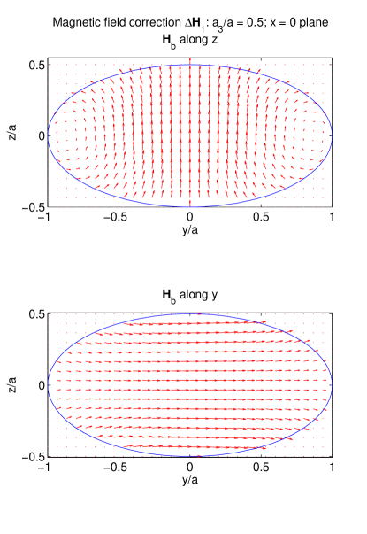
Figure 1: (Color online) Leading magnetic field correction (141) in the $yz$-plane for a spheroid, $a_{1}=a_{2}\equiv a$, using aspect ratio $a_{3}/a=0.5$. Upper plot: background field (139) taken along the $z$-axis. Lower plot: background field taken along the $y$-axis. In both cases, for $x=0$ the field also lies in the $yz$-plane. For background field along $x$ (not shown), the field in this plane is along $x$ as well.

Applying the results of Sec. V [specifically, (V) and the first line of (107) with $n=1$], one obtains the leading correction

$$\Delta{\bf E}_{1} = a_{\alpha}a_{\beta}v({\bf a})$$

$$\times \hat{\cal P}_{\sigma}\left\{x_{\alpha}{\bf\hat{e}}_{\beta}\left[A_{{\bf\hat{e}}_{\alpha}}({\bf a},0)-\sum_{\nu}A_{{\bf\hat{e}}_{\nu}+{\bf\hat{e}}_{\alpha}}({\bf a},0)x_{\nu}^{2}\right]\right.$$

$$- \left.x_{\beta}{\bf\hat{e}}_{\alpha}\left[A_{{\bf\hat{e}}_{\beta}}({\bf a},0)-\sum_{\nu}A_{{\bf\hat{e}}_{\nu}+{\bf\hat{e}}_{\beta}}({\bf a},0)x_{\nu}^{2}\right]\right\}.$$

The projection operator (especially applied to the cubic terms) is very messy, and its result will not be displayed here. However, since it subtracts only a gradient, the curl of (LABEL:7.14) directly produces the leading correction to the magnetic field:

$$\Delta{\bf H}_{1} = \frac{1}{ik\mu}\nabla\times\Delta{\bf E}_{1}$$ (141)

$$= \frac{a_{\alpha}a_{\beta}v({\bf a})}{ik\mu}\Big{(}{\bf\hat{e}}_{\gamma}\big{\{}A_{{\bf\hat{e}}_{\alpha}}({\bf a},0)+A_{{\bf\hat{e}}_{\beta}}({\bf a},0)$$

$$-\ [A_{{\bf\hat{e}}_{\alpha}+{\bf\hat{e}}_{\beta}}({\bf a},0)+3A_{2{\bf\hat{e}}_{\alpha}}({\bf a},0)]x_{\alpha}^{2}$$

$$-\ [A_{{\bf\hat{e}}_{\alpha}+{\bf\hat{e}}_{\beta}}({\bf a},0)+3A_{2{\bf\hat{e}}_{\beta}}({\bf a},0)]x_{\beta}^{2}$$

$$-\ [A_{{\bf\hat{e}}_{\alpha}+{\bf\hat{e}}_{\gamma}}({\bf a},0)+A_{{\bf\hat{e}}_{\beta}+{\bf\hat{e}}_{\gamma}}({\bf a},0)]x_{\gamma}^{2}\big{\}}$$

$$+\ 2x_{\gamma}[A_{{\bf\hat{e}}_{\alpha}+{\bf\hat{e}}_{\gamma}}({\bf a},0)x_{\alpha}{\bf\hat{e}}_{\alpha}$$

$$\ \ \ \ \ \ +\ A_{{\bf\hat{e}}_{\beta}+{\bf\hat{e}}_{\gamma}}({\bf a},0)x_{\beta}{\bf\hat{e}}_{\beta}]\Big{)},$$

in which, again, $(\alpha\beta\gamma)$ is cyclic permutation of $(123)$. It is easily verified that this correction is divergence-free, as required. Example field patterns are shown in Fig. 1 for the case of an oblate spheroid (discus-shape), where the required $A$-coefficients are computed in closed form using the results in Sec. VI.

It is clear that the complexity of the polynomial form $\Delta{\bf E}_{n}$ increases rapidly with $n$, and a numerical implementation is required to keep track of all the terms. In later sections we will show theoretical results, and comparisons to experiment, using all 232 basis functions with $l+2p\leq 7$, where convergence is found even when $\eta_{s}$ is not small.

VII.3 External field

It is the field external to the scatterer that is relevant to target detection. Equation (21) allows computation of (the inductive part of) the external field once the internal field is known foot:noninductext . Specifically, from the series (136), one obtains

$${\bf E}^{(\mathrm{ind})}_{\mathrm{ext}}({\bf x})\equiv ik{\bf A}({\bf x})=\sum_{n=0}^{\infty}\left(\frac{ik\mu\sigma}{c}\right)^{n}\Delta{\bf E}^{(\mathrm{ind})}_{n}({\bf x})$$ (142)

in which $\Delta{\bf E}_{0}^{(\mathrm{ind})}=ik{\bf A}_{b}$ is the inductive part of the background field (both inside and outside the target), and

$$\Delta{\bf E}^{(\mathrm{ind})}_{n}({\bf x})=\int_{V_{s}}d^{3}x^{\prime}\frac{\Delta{\bf E}_{n-1}({\bf x}^{\prime})}{|{\bf x}-{\bf x}^{\prime}|},\ {\bf x}\notin V_{s},\ n\geq 1.$$ (143)

If the result for $\Delta{\bf E}_{n-1}$ is a polynomial, as described in Sec. VII.2, then the results of Sec. V directly produce the external field in the form of sum of products of polynomials with elliptic functions. The latter are now functions of position ${\bf x}$ via the nonzero value of $\lambda({\bf x})$—see (73).

For example, the linear form (138) for the background field produces a leading correction

$$\Delta{\bf E}^{(\mathrm{ind})}_{1} = a_{\alpha}a_{\beta}v({\bf a})$$

$$\times \left\{x_{\alpha}{\bf\hat{e}}_{\beta}\left[A_{{\bf\hat{e}}_{\alpha}}({\bf a},\lambda)-\sum_{\nu}A_{{\bf\hat{e}}_{\nu}+{\bf\hat{e}}_{\alpha}}({\bf a},\lambda)x_{\nu}^{2}\right]\right.$$

$$- \left.x_{\beta}{\bf\hat{e}}_{\alpha}\left[A_{{\bf\hat{e}}_{\beta}}({\bf a},\lambda)-\sum_{\nu}A_{{\bf\hat{e}}_{\nu}+{\bf\hat{e}}_{\beta}}({\bf a},\lambda)x_{\nu}^{2}\right]\right\},$$

which is identical in form to (LABEL:7.14), but with the projection operator omitted, and now including nonzero $\lambda$.

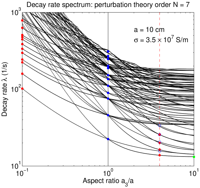
Figure 2: (Color online) Spheroid decay rate spectrum vs. aspect ratio $\alpha=a_{3}/a$, with conductivity $\sigma$ and radius $a$ fixed as indicated. Unit permeability, $\mu=\mu_{b}=1$, is used as well. The first 125 decay rates (out of a total of 232 that are computed using all 232 basis functions with order $N=l+2p\leq 7$) are plotted for each $0.1\leq\alpha\leq 10$. Apparent sharp bends in the curves at the top of the spectrum are artifacts of this truncation. Blue dots at $\alpha=1$ show exact analytic results for the sphere, with degeneracy effects from enhanced symmetry evident. Red dots at $\alpha=4$ mark the four (doubly degenerate) vertically circulating modes shown in Fig. 3; blue circles mark the four azimuthally circulating modes shown in Fig. 4. The green dot at the right is the analytic result for the lowest mode for an infinite cylinder, $\alpha\to\infty$. More slowly increasing branches at the left, $\alpha\ll 1$, correspond to modes with current patterns circulating in the $xy$-plane. The red dots at $\alpha=0.1$ mark the first twelve such modes shown in Fig. 5.

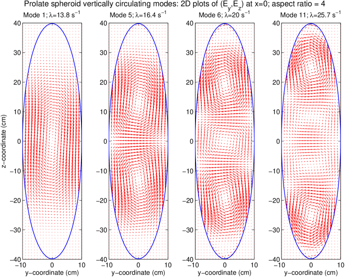
Figure 3: (Color online) Four lowest order vertically circulating mode shapes, and corresponding decay rates (red dots at $a_{3}/a=4$ in Fig. 2), for a $10\times 10\times 40$ cm radius aluminum prolate spheroid: $(E_{y},E_{z})$ are plotted in the $x=0$ plane (where $E_{x}$ vanishes identically).

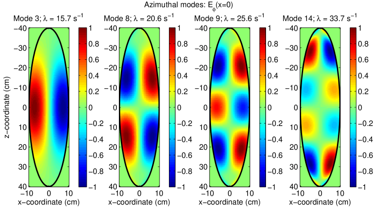
Figure 4: (Color online) Four lowest order azimuthally circulating mode shapes, and corresponding decay rates (blue circles at $a_{3}/a=4$ in Fig. 2), for a $10\times 10\times 40$ cm radius aluminum prolate spheroid. The azimuthal component of the electric field $E_{\phi}$ (or $E_{x}$), normalized by its maximum magnitude, is plotted in the $x=0$ plane; all other components vanish. Currents in the lowest mode (far left) circulate in the same direction at all heights. As the mode order increases (from left to right), the number of nodal surfaces, across which the circulation direction of the current changes sign, increases.

VII.4 Far-field asymptotics: multipole expansion

Computation of the external field greatly simplifies if one is far from the target—greater than a few maximum target radii, say—but not so far that non-quasistatic corrections to the Green function (6) become important.

First, for large $|{\bf x}|/L_{s}$ the cubic equation (73) for $\lambda$ has the expansion

$$\lambda({\bf x})=|{\bf x}|^{2}-\sum_{\alpha}a_{\alpha}^{2}\hat{x}_{\alpha}^{2}+O(1/|{\bf x}|^{2}),$$ (145)

in which ${\bf\hat{x}}={\bf x}/|{\bf x}|$ is the unit vector with components $\hat{x}_{\alpha}=x_{\alpha}/|{\bf x}|$. For large $\lambda$ one finds in turn,

$$A_{\bf k}({\bf a},\lambda) = \int_{\lambda}^{\infty}\frac{dt}{t^{|{\bf k}|+3/2}}\frac{1}{\prod_{\alpha}(1+a_{\alpha}^{2}/t)^{k_{\alpha}+1/2}}=\int_{\lambda}^{\infty}\frac{dt}{t^{|{\bf k}|+3/2}}\left[1-\frac{1}{2t}\sum_{\nu}(2k_{\alpha}+1)a_{\alpha}^{2}+O(1/t^{2})\right]$$ (146)

$$= \frac{2}{2|{\bf k}|+1}\frac{1}{\lambda^{|{\bf k}|+1/2}}-\frac{\sum_{\alpha}(2k_{\alpha}+1)a_{\alpha}^{2}}{2|{\bf k}|+3}\frac{1}{\lambda^{|{\bf k}|+3/2}}+O\left(\frac{1}{\lambda^{|{\bf k}|+5/2}}\right),$$

with, as before, $|{\bf k}|=\sum_{\alpha}k_{\alpha}$. Substituting (145), one obtains explicitly

$$A_{\bf k}({\bf a},\lambda)=\frac{2}{2|{\bf k}|+1}\frac{1}{|{\bf x}|^{2|{\bf k}|+1}}+\left[\sum_{\alpha}a_{\alpha}^{2}\hat{x}_{\alpha}^{2}-\frac{\sum_{\alpha}(2k_{\alpha}+1)a_{\alpha}^{2}}{2|{\bf k}|+3}\right]\frac{1}{|{\bf x}|^{2|{\bf k}|+3}}+O\left(\frac{1}{|{\bf x}|^{2|{\bf k}|+5}}\right).$$ (147)

As an example, leading behavior of the external field correction (LABEL:7.18) takes the simple magnetic dipole form

$$\Delta{\bf E}^{(\mathrm{ind})}_{1}=\frac{4a_{\alpha}a_{\beta}v({\bf a})}{15|{\bf x}|^{2}}\left(\hat{x}_{\alpha}{\bf\hat{e}}_{\beta}-\hat{x}_{\beta}{\bf\hat{e}}_{\alpha}\right).$$ (148)

Higher order terms in (142) will generally all have a leading $1/|{\bf x}|^{2}$ term, but with more complicated angular dependence. This may be formalized via a vector multipole expansion using the vector harmonics (37) Jackson .

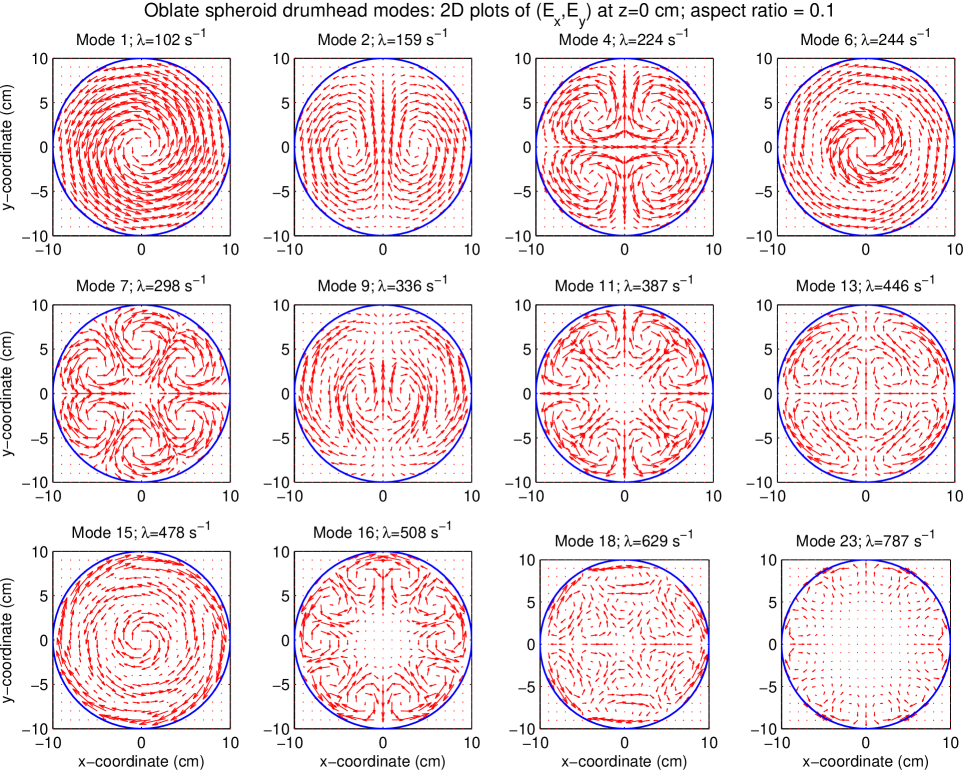
Figure 5: (Color online) Twelve lowest order horizontal circulating “drumhead” mode shapes, and corresponding decay rates (red dots at $a_{3}/a=0.1$ in Fig. 2), for a $20\times 20\times 2$ cm radius aluminum prolate spheroid: $(E_{x},E_{y})$ are plotted in the $z=0$ plane (where $E_{x}$ vanishes). Modes 1,6,15 have azimuthal symmetry (angular momentum index $m=0$) and are non-degenerate. The remainder, with $m>0$, are doubly degenerate, with the second mode shape obtained via a $\pi/2m$ rotation about the $z$-axis (modes 2,9 have $m=1$; modes 4,13 have $m=2$; modes 7,18 have $m=3$; mode 11 has $m=4$; mode 16 has $m=5$; mode 23 has $m=6$). For fixed $m$, the higher order modes have increasingly complex radial structure, with the circulation direction changing sign with radius (see modes 6,9,13,15,18).

VIII Time domain response

Having presented the general theory, and some leading order perturbation results in the previous sections, we now turn to more sophisticated applications of the theory that require numerical implementation of high order expansions in $\eta_{s}$. Specifically, theoretical predictions for time-domain EM measurements will now presented (see Secs. I.2 and II.4) and compared to experimental data. As described previously, time domain measurements are those of the freely decaying response of a target after termination of an applied pulse.

Any time-domain response may, of course, be written as the Fourier superposition of a spectrum of frequency domain responses, each of which may be individually computed using the previous theory. However, as will be described below, the formulation in terms of a superposition of freely decaying modes, equation (1), is numerically more efficient because these need only be computed once for a given target, avoiding recomputation of the perturbation series for each of a continuous set of frequencies. In fact, these modes can be used to directly solve the frequency domain problem as well.

A more important point is that a rapidly terminated pulse (over tens of microseconds, in the experiments to be analyzed further below) has a spectrum that includes some very high frequencies (e.g., tens of kHz), for which $\eta$ is a far larger than can be handled at any achievable order in perturbation theory. However, this part of the spectrum mainly excites very rapidly decaying modes that disappear from the later-time domain response. Thus, the mode approach allows accurate prediction of the signal at later time even when it fails at earlier time. In fact, the very large number of modes appearing at early-time make it a poor representation of the response. A complementary description in terms of the inward diffusion of screening surface currents W2003 ; W2004 should be used instead. It will be seen below that a merging of the two theories provides a complete description of the signal.

VIII.1 Mode computation

The freely decaying mode computation is implemented via the generalized eigenvalue equation (45). Specifically, the modes are written as a superposition (44) of the truncated set of vector harmonic modes (II.3.2), rescaled according to (34), with $l+2p\leq N$ for some chosen upper limit $N$. Results will be shown for $N=7$ (which yields a total of 232 basis functions—116 for each type $i=1,2$), which will be seen to suffice for accurate comparison with experiment. Since ${\bf Z}_{lmp}^{({\bf a};i)}({\bf x})$ is a polynomial of degree $l+2p+i-1$, the ${\bf x}^{\prime}$ integral defining the $H$-matrix (31) produces, via the results of Sec. V, a polynomial of degree $l+2p+i+1$. The final ${\bf x}$ integral [which, it should be recalled, automatically implements the projection operator $\hat{\cal P}_{\sigma}$ in (26) and (43)], in both (31) and the definition of the $O$-matrix (30) (with uniform $\sigma$ here) is then a pure polynomial integral, and is trivial.

Figure 2 show results for the decay rate spectrum of a range of spheroids ($a_{1}=a_{2}\equiv a$). The lowest 125 decay rates (out of a total of 232 computed at this at order $N=7$) are plotted for each of 201 aspect ratios $\alpha=a_{3}/a$ in the range $0.1\leq\alpha\leq 10$. Even though these are plotted for a particular choices of radius and conductivity (as well as permeability), in the high contrast limit the combination $\lambda\mu\sigma a^{2}$ is independent of all three. Hence these results may be trivially rescaled to obtain results for any spheroid with the same geometry. The mode eigenfunctions scale trivially with $a$ as well. Note as well that the azimuthal symmetry (which is exactly preserved in by the perturbation theory at fixed $N$) means that the $z$ angular momentum index $m$ is a “good quantum number”, making the matrices $O$ and $H$ block diagonal. The eigenvales for $\pm m$ are also degenerate, so that many of the lines in Fig. 2 actually represent pairs of modes.

Exact results for the sphere, at $\alpha=1$, are shown by cyan dots, and indicate the accuracy of the method for rather large effective values of $\eta_{s}=O(10)$ [obtained by substituting $a$ for $L_{s}$ and $\lambda$ for $f$ in (134)]. The total angular momentum index $l$ is now also a good quantum number, and the vast increase in degeneracy is evident.

The infinite right circular cylinder of radius $a$ corresponds to $\alpha\to\infty$. In this limit, translation invariance implies that the $z$-dependence of the modes is given by $e^{ikz}$ for arbitrary wavenumber $k$. The analytic result for one of the $k=0$ modes (with current traveling up one side of the cylinder and down the other), is shown as the green dot, and is seen to have converged even at $\alpha=10$.

A few mode shapes for the prolate spheroid with $\alpha=4$ are illustrated in Figs. 3 and 4. The four modes in Fig. 3, consisting of an increasing number of vortices circulating in the $yz$-plane and indicated by the red dots in Fig. 2, are doubly degenerate (with the second mode obtained by $90^{\circ}$ rotation about the $z$-axis). One may think of these modes as approximating those of an infinite cylinder with $k\approx n\pi/a_{3}$, $n=1,2,3,4$.

The modes shown in Fig. 4, indicated by the blue circles in Fig. 2, are non-degenerate. Here the current always circulates in the $xy$-plane, but the flow direction oscillates with $z$. Again, they may be thought of in terms of those of an infinite cylinder with $k\approx n\pi/a_{3}$, $n=1,2,3,4$.

A set of twelve modes for an oblate spheroid, with aspect ratio $\alpha=0.1$ are shown in Fig. 5. As seen Fig. 2, since the radius $a$ is fixed, the mode decay rates increase as they become vertically “squeezed” by decreasing $a_{3}$. We denote these “drumhead modes” because a plot of the vertical component of the magnetic field $H_{z}=\partial_{x}E_{y}-\partial_{y}E_{z}$ would look very similar to the surface height pattern of a vibrating drumhead. Of course, the latter oscillate at fixed frequency, rather than relax exponentially, but there are parallels in the physics of the underlying mode patterns.

There are two independent time scales that operate to determine the scaling of $\lambda$ with $a_{3}$ for a particular mode pattern, and the interplay between them basically determines the shapes of the curves in Fig. 2.

For a circulating current vortex that is very thin (the dimension $a_{3}$ for the modes in Fig. 5) compared to its horizontal extent (the dimension $a_{v}$ of one of the individual vortices in the mode current pattern), the decay is dominated the decay of stored magnetic energy via Joule heating. Thus, the dissipated power scales as $P=I^{2}R\sim(Ja_{v}a_{3})^{2}/(\sigma a_{3})=J^{2}a_{v}^{2}a_{3}/\sigma$, where $J$ is the characteristic current density. The magnetic energy is estimated as $U_{H}=\mu B^{2}V_{\mathrm{eff}}$, in which $B\sim I/ca_{v}=Ja_{3}/c$ is the magnetic field within a circulating current field and $V_{\mathrm{eff}}\sim a_{v}^{3}$ is the effective volume over which it is supported (mostly outside the target when $a_{3}/a_{v}\ll 1$), then scales as $U_{H}\sim J^{2}a^{3}a_{3}^{2}/c^{2}$ foot:ring . The ratio $\lambda\sim P/U_{H}\sim c^{2}/\sigma\mu aa_{3}=c^{2}/\sigma\mu a^{2}\alpha$, as claimed. For the modes in Fig. 2, $a_{v}/a$ remains roughly fixed as $a_{3}/a\to 0$, and this produces the observed $\lambda\sim 1/\alpha$ scaling for $\alpha\ll 1$.

On the other hand, if two oppositely oriented currents streams lie very close to each other, the decay is dominated by transverse diffusion of the streams into each other, which causes them to cancel out. The diffusion time scale is $\tau_{D}\sim Dd^{2}$, where $d$ is the current stream separation,

$$D=\frac{c^{2}}{4\pi\sigma\mu}$$ (149)

is the diffusion constant, and one estimates $\lambda\sim 1/\tau_{D}\sim c^{2}/\mu\sigma d^{2}$. For modes with alternating current sheets in the vertical dimension one has $d\propto a_{3}$ (e.g., the mode geometries pictured in Figs. 3 or 4, where $d/a_{3}\approx n$ for $n=1,2,3,4$, but squeezed in the vertical dimension), and this leads to the $\lambda\sim 1/\alpha^{2}$ scaling seen for the steeper curves on the left side of Fig. 2.

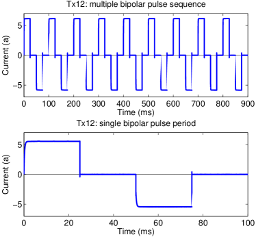
Figure 6: (Color online) Transmitter pulse train generated by the NRL-TEMTADS platform. The pulse train (with maximum current approximately 5.7 a), is bipolar, meaning that it consists of identical pulses of alternating sign. The average current is then zero, which helps average out certain transients. The leading edge of each pulse is actually a sequence of three exponential relaxations, with time constants of 2.5 $\mu$s, 0.33 ms, and 4 ms. The trailing edge is a linear offramp over a 10 $\mu$s interval. The total length of both the pulse and the following quiescent detection interval is 25 ms.

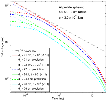
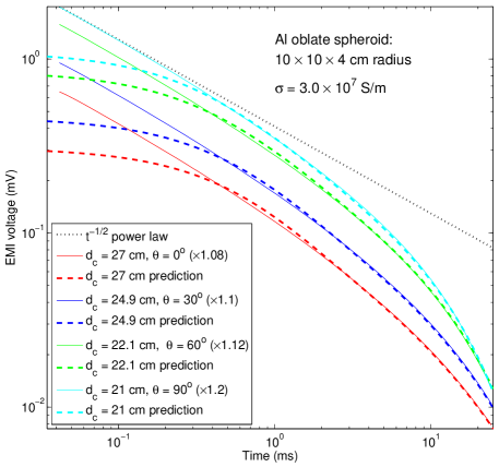
Figure 7: (Color online) Comparisons of data (solid lines; taken by the NRL-TEMTADS platform TEMTADS ; foot:temtads ) and ab initio theoretical predictions (dashed lines) for a $5\times 5\times 10$ cm radius aluminum prolate spheroid (left) and a $10\times 10\times 4$ cm radius aluminum oblate spheroid (right), at various depths-to-center $d_{c}$, with various axial tilt angles $\theta$. The target is centered under the transmitter-receiver pair. Plotted are the measured receiver voltages beginning immediately after the pulse termination times seen in Fig. 6, averaged over about ten cycles. The multipliers indicated in each legend entry reflect a $\sim 10$% variability in the transmitter current, as well as residual coil characterization foot:temtads and target positioning errors, and are applied to the data to optimize the fit. Straight dashed lines show the predicted $1/\sqrt{t}$ early time divergence W2003 . This first principles agreement, over nearly two decades in both time and voltage, is remarkable.

VIII.2 Comparisons with experimental data

VIII.2.1 Mode excitation and voltage amplitude computation

Having explored some details of the mode physics, we now illustrate, through comparisons with experimental data on artificial aluminum spheroids, how the mode theory is used to compute measurable quantities through incorporation of a detailed model of the measurement platform.

The first step is to relate the excitation coefficients $A_{n}$ in the free decay series (1) to the source excitation pulse, encoded in ${\bf S}$ on the right hand side of the wave equation (5). In the time domain, this equation reads

$$\frac{1}{D({\bf x})}\partial_{t}{\bf E}({\bf x},t)+\nabla\times\nabla\times{\bf E}({\bf x},t)=-\frac{4\pi\mu}{c^{2}}\partial_{t}{\bf j}_{S}({\bf x},t).$$ (150)

One seeks the solution in the form

$${\bf E}({\bf x},t)=\sum_{n}{\cal A}_{n}(t){\bf e}^{(n)}({\bf x})$$ (151)

generalizing (1). Substituting this into (150), and using the mode defining relation (42) and the orthogonality condition (47), one obtains the equation of motion for the individual amplitudes:

$$(\partial_{t}+\lambda_{n}){\cal A}_{n}=-\partial_{t}j_{n}$$ (152)

where

$$j_{n}(t)=\int d^{3}x{\bf e}^{(n)^{*}}({\bf x})\cdot{\bf j}_{S}({\bf x},t)$$ (153)

is the inner product of the source current with the mode eigenfunction. For a compact transmitter loop ${\cal C}_{T}$ with $N_{T}$ windings carrying current $I_{T}(t)$ (see Fig. 6 for an example), this reduces to the line integral foot:lineint

$$j_{n}(t) = N_{T}a_{n}I_{0}(t)$$

$$a_{n} \equiv \oint_{{\cal C}_{T}}{\bf e}^{(n)*}({\bf x})\cdot d{\bf l}$$ (154)

The solution to (152) is

$${\cal A}_{n}(t) = N_{T}a_{n}I_{n}(t)$$

$$I_{n}(t) \equiv -\int_{-\infty}^{t}dt^{\prime}e^{-\lambda_{n}(t-t^{\prime})}\partial_{t^{\prime}}I_{0}(t^{\prime})$$ (155)

$$= I_{n}(t_{p})e^{-\lambda_{n}(t-t_{p})},$$

where the second line is valid during any quiescent interval following the termination of a pulse at time $t_{p}$. Note that for a very sharp pulse termination, on a time-scale shorter than $1/\lambda_{n}$, one may approximate $-\partial_{t^{\prime}}I_{0}(t^{\prime})\simeq\Delta I_{0}\delta(t-t_{p})$, where $\Delta I_{0}$ is the down-step size (e.g., about 5 a in Fig. 6). The termination then contributes $\Delta I_{0}$ to $I_{n}(t_{p})$. In any case, it follows that the required coefficient in (1) is given by

$$A_{n}={\cal A}_{n}(t_{p})=N_{T}a_{n}I_{n}(t_{p})$$ (156)

For a compact receiver loop ${\cal C}_{R}$ with $N_{R}$ windings, the voltage is given by the line integral

$$V(t)=N_{R}\oint_{{\cal C}_{R}}{\bf E}({\bf x},t)\cdot d{\bf l}.$$ (157)

Substituting (151), one obtains the voltage series (2) with

$$V_{n}=A_{n}N_{R}b_{n}=N_{T}N_{R}a_{n}b_{n}I_{n}(t_{p})$$ (158)

where

$$b_{n}=\oint_{{\cal C}_{R}}{\bf e}^{(n)}({\bf x})\cdot d{\bf l}.$$ (159)

is the corresponding receiver loop line integral.

This completes the specification of the measured voltage in terms of modal quantities given the transmitter and receiver loop characteristics. Note that computation of $a_{n}$ and $b_{n}$ requires evaluation of the external electric field. For this purpose, the right hand side of (43) is evaluated using the previously computed internal forms (44) for the mode eigenfunctions. This evaluation requires the various quantities worked out in Sec. V for positive values of the parameter $\lambda({\bf x})$. The far field asymptotic forms described in (VII.4) may be used at sufficient target standoff. The line integrals defining $a_{n},b_{n}$ are then performed numerically numrec through evaluations at a discrete set of points along the loops ${\cal C}_{T},{\cal C}_{R}$ foot:rotate . The pulse wave forms $I_{0}(t)$ are typically given by a sequence of relaxing exponentials and linear ramps, for which $I_{n}(t)$ may be evaluated analytically foot:multipulse .

All of these algorithms have been implemented numerically to produce the comparisons now described. Given the precomputation of the mode properties (which requires 10–20 minutes for a given target on a standard workstation), computation of the voltage series (2) is found to take only about 1 s. This speed is critical to efficient solution inverse problems which underlie, for example, the UXO discrimination problem. For the latter, properties of an unknown target are estimated by searching over different candidate targets to find the one that produces the best fitting voltage curve predictions foot:inverse .

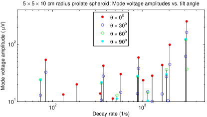
Figure 8: Plot of the largest individual mode voltage amplitudes $V_{n}$ in the series (2), plotted vs. mode decay rate $\lambda_{n}$, corresponding to the time-domain curves in Fig. 7 (top: prolate spheroid; bottom: oblate spheroid). Of particular note is the complete complementarity of the excited modes for vertical ($\theta=0^{\circ}$; red dots) and horizontal ($\theta=90^{\circ}$; blue dots) targets, which is primarily responsible for the decay rate of the curves at later time. A mixture of the two sets is excited at intermediate tilt angles (blue and green circles). It is the the failure of the amplitudes to decrease with increasing decay rate that is responsible for the diverging signals at early time.

VIII.2.2 Comparison with NRL-TEMTADS measurements

In Fig. 7 we show comparisons between the theory and data taken on artificial aluminum spheroids using the Naval Research Labs TEMTADS platform TEMTADS . The platform consists of a $5\times 5$ horizontal array of 25 independent, well calibrated, high dynamic range concentric transmitter and receiver coils. The coils are square ($35\times 35$ cm, with $N_{T}=35$ windings for the transmitters; $25\times 25$ cm, with $N_{R}=16$ windings, for the receivers) and laid out flat in the same plane with 40 cm between centers in each direction foot:temtads . The pulse waveform is described in Fig. 6. For illustrative purposes, only the strongest signal, from the coil under which the target was centered, is shown in Fig. 7 foot:inverse .

The data quality is seen to be very high, with no visible noise or distortion over more than two decades dynamic range of voltage and time. The model predictions (dashed lines) are seen to very accurately reproduce the data, except at very early time where, as explained earlier, the absence of the contribution of more complex modes in the series (2) with decay times faster than about 0.25 ms ($\lambda_{n}\gtrsim 4000$ s^-1) cause them to fall below the data curves (solid lines). In comparison, the fundamental modes here are a few tens of inverse seconds, (as can read off Fig. 2 for $a_{3}/a=2,0.4$ after applying the $1/\sigma a^{2}$ scaling), and hence have decay times comparable to the extent of the 25 ms measurement window. However, as also noted previously, the early time portion of the data follows the predicted $1/\sqrt{t}$ divergence (ultimately cut off only by the finite 10 $\mu$s pulse off-ramp width, which lies invisibly below the TEMTADS measurement window) W2003 . Significantly, the $N=7$th order mean field prediction succeeds in overlapping this regime, so that by simply substituting a $V_{\mathrm{pred}}(t*)\sqrt{t^{*}/t}$ tail to the early time prediction (below an optimally chosen crossover time $t^{*}\sim 0.25$ ms), one obtains a model fit to the that is accurate (at the $\sim 5$% level) over the entire dynamic range of the data.

The different curves in Fig. 7 correspond to a combination of different target depths and orientations. The changing depth-to-center $d_{c}$ has week effect on the shape of the curves, mainly changing the overall amplitude (with a roughly $1/d_{c}^{6}$ dipolar dependence). This is a reflection of the fact that, at these standoffs and for a centered target, the applied magnetic field in the target region is fairly uniform and vertical.

The effect of orientation is more interesting, visibly changing the steepness of the curves at later time, with the oblate spheroid (right panel) showing a stronger effect of this type than the prolate spheroid (left panel). The reason for this (as quantified in Fig. 8, which shows a plot of the individual mode amplitudes) is that for a vertical symmetry axis ($\theta=0$), it is horizontally circulating modes of the type shown in Figs. 4 and 5 that are most strongly excited [consistent with the line integrals (154), (159)], whereas for a horizontal symmetry axis it is the vertically circulating modes, of the type shown in Fig. 3). Looking at Fig. 2 (and also the upper panel in Fig. 8), one sees that for $a_{3}/a>1$ the leading vertical mode (curve containing the lowest red dot) decays slightly more slowly than the leading horizontal mode (curve containing the lowest blue circle). This explains why the red curve ($\theta=0^{\circ}$) in the left panel of Fig. 7 is slightly steeper at late time than the cyan curve ($\theta=90^{\circ}$). Conversely, for $a_{3}/a<1$, it is the horizontal modes that are more slowly decaying (see also the lower panel in Fig. 8), and the decay rate gap is much larger (diverging as $a_{3}/a\to 0$). This explains why, in the right panel, the cyan curve is significantly steeper at late time than the red curve.

There is no distinction between the shapes of the curves at early time, other than the overall amplitude of the $1/\sqrt{t}$ divergence. However, the behavior of the amplitudes in Fig. 8 with increasing decay rate explains the origin of this divergence in the mode picture. As shown in Ref. W2003 , immediately after pulse termination, the currents form a very thin sheet on the target surface. The delta-function-like feature requires a superposition of an essentially infinite number of modes (cut off only by the ultimately finite pulse off-ramp rate), and one indeed sees in Fig. 8 that the mode amplitudes, if anything, are actually growing with increasing decay rate. In fact, as can be seen explicitly in the exact solution for the sphere, there is an infinite subset of modes (corresponding there to a fixed subset angular momentum indices $l,m$ that depend on the geometry of the background exciting field) which have asymptotically constant excitation $V_{0}$, and make a voltage contribution

$$V(t)\approx V_{0}\sum_{p=p_{0}}^{\infty}e^{-\lambda_{0}p^{2}t}\approx V_{0}\sqrt{\frac{\pi}{4\lambda_{0}t}},\ t\to 0,$$ (160)

where $\lambda_{0}\sim 1/\mu\sigma a^{2}$ describes the asymptotic behavior of the decay rates for large enough $p\geq p_{0}$. Equivalently, one expects, for a general target with a sufficiently regular surface, that there is a density of states $\rho_{e}(\lambda)\sim 1/\sqrt{\lambda}$ [a small fraction of the total, which increases as $\rho_{\mathrm{tot}}(\lambda)\sim\sqrt{\lambda}$], with constant excitation for large $\lambda$, which indeed leads to $V(t)\sim\int\rho_{e}(\lambda)e^{-\lambda t}d\lambda\sim 1/\sqrt{t}$ for $t\to 0$.

It is observations such as those above, connecting the geometry of the decay curves to the geometry of the target, that are critical to a workable inversion scheme foot:inverse . It is also clear how data from multiple sensors, or from different platform positions, which see different effective orientations of the target, can greatly aid in such an effort.

As a final comment, the quality of the fits points to an interesting implication regarding the accuracy of the higher order mode contributions. It is apparent from the exact sphere comparison (blue dots) in Fig. 2 that the decay rates, and presumably the mode shapes, can be trusted quantitatively only, perhaps, for the first few dozen modes (recall, also, that this figure shows only the first 125 out of 232 computed modes). However, it is clear that their summed contribution to the induced voltage measurement is quantitatively extremely accurate. This points to the conclusion that the overall effect of a group of modes with similar decay rates (in a density of states sense) depends only on the part of the mode Hilbert space that they cover, not on the detailed partitioning of that subspace between individual modes. One can imagine a very complex applied field, generated by an intricate set of transmitter coils surrounding the entire target that is tuned to excite a single high order mode, for which the prediction will badly fail. However, for the relatively uniform fields of interest here, the conclusion appears valid.

IX Generalizations of the theory

In this final section we describe various generalizations of the basic theory. In Sec. IX.1 we consider permeable targets, $\mu\neq\mu_{b}$. In Sec. IX.2 we consider simplifications in the high contrast limit $\mu/\mu_{b}\gg 1$, relevant to ferrous targets where $\mu/\mu_{b}=O(10^{2})$. The high magnetic contrast limit parallels in many ways that of the high conductivity contrast limit (e.g., it enforces a vanishing surface normal ${\bf\hat{n}}\cdot{\bf H}$ of the internal magnetic field). However, there are some surprising subtleties in the external field computation, which is shown to vanish when $\mu_{b}/\mu\to 0$. A computation of the leading $O(\mu_{b}/\mu)$ dependence of ${\bf\hat{n}}\cdot{\bf H}$ is then required, and we show how to accomplish this within the Chandrasekhar formalism. In Sec. IX.3 we consider the computation of the freely decaying eigenmodes. Unlike in the nonmagnetic case (Sec. II.4) where the eigenmodes follow trivially from the diagonalization of the Coulomb integral operator (43), in the magnetic case the frequency dependence enters the operator in a more complicated way, and a sequential search must be performed to find the decay rates. In Sec. IX.4 we consider more realistic target geometries, including hollow targets and multiple targets. Finally, in Sec. IX.5 we consider the effects of background permeability variations. We have shown that background conductivity variations do not impact an induction measurement, but even a very small background permeability has a strong impact.

All of these generalizations require significantly more work to implement, and their applications to experimental data will therefore be described elsewhere.

IX.1 Generalization to inhomogeneous permeability

For inhomogeneous permeability, (5) is replaced by,

$$\mu_{b}\nabla\times\left(\frac{1}{\mu_{b}}\nabla\times{\bf E}_{b}\right)-\kappa_{b}^{2}{\bf E}_{b} = {\bf S}$$

$$\mu\nabla\times\left(\frac{1}{\mu}\nabla\times{\bf E}\right)-\kappa^{2}{\bf E} = {\bf S}.$$ (161)

Subtracting the first equation from the second, one obtains

$$\nabla\times\left[\frac{1}{\mu_{b}}\nabla\times({\bf A}-{\bf A}_{b})\right] = \frac{1}{ik\mu_{b}}\left[\kappa^{2}{\bf E}-\kappa_{b}^{2}{\bf E}_{b}\right]$$ (162)

$$+\ \left(\nabla\frac{\mu}{\mu_{b}}\right)\times{\bf H},$$

in which the magnetic field has been introduced via ${\bf H}={\bf B}/\mu=(ik\mu)^{-1}\nabla\times{\bf E}$, and we have again represented the electric field in the form (12), (13) in terms of a Coulomb gauge vector potentials and the gradient of a scalar potential. We now define the background quasistatic (symmetric) tensor Green function ${\bf G}_{A}({\bf x},{\bf x}^{\prime})$ by

$$\nabla\times\left[\frac{1}{\mu_{b}}\nabla\times{\bf\hat{G}}_{A}({\bf x},{\bf x}^{\prime})\right] = {\bf\hat{P}}_{T}\delta({\bf x}-{\bf x}^{\prime})$$

$$\nabla\cdot{\bf\hat{G}}_{A}({\bf x},{\bf x}^{\prime}) = 0,$$ (163)

in which ${\bf\hat{P}}_{T}=\delta({\bf x}-{\bf x}^{\prime})\openone+\nabla\nabla(4\pi|{\bf x}-{\bf x}^{\prime}|)^{-1}$ is the transverse (divergence-free) projection of the delta function. One obtains the formal solution

$${\bf A}({\bf x})-{\bf A}_{b}({\bf x}) = \int d^{3}x^{\prime}{\bf\hat{G}}_{A}({\bf x},{\bf x}^{\prime})\cdot\left\{\left(\nabla\frac{\mu}{\mu_{b}}\right)\times{\bf H}({\bf x}^{\prime})\right.$$ (164)

$$+ \left.\frac{1}{ik\mu_{b}}\left[\kappa^{2}{\bf E}({\bf x}^{\prime})-\kappa_{b}^{2}{\bf E}_{b}({\bf x}^{\prime})\right]\right\}.$$

The Green function ${\bf\hat{G}}_{A}$ accounts explicitly for variations in the background permeability, and in the non-magnetic limit (164) reduces to (20). Analytic forms for ${\bf\hat{G}}_{A}$ also exist, e.g., for horizontally stratified backgrounds. Since $\mu/\mu_{b}$ is typically discontinuous at the target boundary it is convenient to eliminate the resulting surface term by integrating the ${\bf H}$ term on the right hand side by parts. One obtains,

$${\bf A}({\bf x})-{\bf A}_{b}({\bf x})=\int d^{3}x^{\prime}\left\{\frac{4\pi}{c}{\bf\hat{G}}_{A}({\bf x},{\bf x}^{\prime})\cdot[\sigma{\bf E}({\bf x}^{\prime})-\sigma_{b}{\bf E}_{b}({\bf x}^{\prime})]+\left(\frac{\mu}{\mu_{b}}-1\right)[\nabla^{\prime}\times{\bf\hat{G}}_{A}({\bf x},{\bf x}^{\prime})]\cdot{\bf H}({\bf x}^{\prime})\right\}$$ (165)

in which the curl operation acts on the second index of ${\bf\hat{G}}_{A}$. So far, no approximations have been made, but in the high contrast limit one may drop the $\epsilon_{b}{\bf E}_{b}$ term and restrict the integral to the target volume $V_{s}$. For uniform $\mu_{b}$ one may replace

$${\bf\hat{G}}_{A}({\bf x},{\bf x}^{\prime})\to\openone\frac{\mu_{b}}{4\pi|{\bf x}-{\bf x}^{\prime}|}.$$ (166)

The transverse projection terms do not contribute because the right hand side of (162), and all terms derived from it in (164) and (165), are divergence free. With these simplifications, (165) now reduces to

$${\bf A}({\bf x})-{\bf A}_{b}({\bf x}) = \frac{4\pi\mu_{b}}{c}\int_{V_{s}}d^{3}x^{\prime}\frac{\sigma({\bf x}^{\prime}){\bf E}({\bf x}^{\prime})}{4\pi|{\bf x}-{\bf x}^{\prime}|}$$

$$+ \nabla\times\int_{V_{s}}d^{3}x^{\prime}\frac{[\mu({\bf x}^{\prime})-\mu_{b}]{\bf H}({\bf x}^{\prime})}{4\pi|{\bf x}-{\bf x}^{\prime}|}.$$

IX.1.1 Coupled integral equations for E and H

One may now, in principle, use (165) or (IX.1) as the basis for a low frequency perturbation theory. However, upon substituting for ${\bf H}$, the appearance of the curl of ${\bf E}$, in addition to ${\bf E}$ itself, on the right hand side is found to decrease numerical stability, and it is preferable to use a more symmetric approach in which ${\bf E}$ and ${\bf H}$ are treated on an equal footing.

One may obtain a second equation coupling the two fields by taking the curl of both sides of (165). However, the left hand side then produces the combination $\mu{\bf H}-\mu_{b}{\bf H}_{b}$ rather than ${\bf H}-{\bf H}_{b}$, which turns out to be less convenient. In order to obtain the latter, we construct an alternative to (161) by formulating the Maxwell equations in terms of ${\bf H}$ instead of ${\bf E}$. One may combine the Maxwell equations for ${\bf H}$ and ${\bf H}_{b}$ in the form

$$\nabla\times({\bf H}-{\bf H}_{b}) = -ik(\epsilon{\bf E}-\epsilon_{b}{\bf E}_{b})$$

$$\nabla\cdot[\mu_{b}({\bf H}-{\bf H}_{b})] = -\nabla\cdot[(\mu-\mu_{b}){\bf H}],$$ (168)

in which the source term has been canceled and the right hand side of the second equation vanishes outside of the target volume $V_{s}$. In order to formulate these as an integral equation, define the magnetic field tensor Green function by

$${\bf\hat{G}}_{H}({\bf x},{\bf x}^{\prime})=\frac{1}{\mu_{b}}\nabla\times{\bf\hat{G}}_{A}({\bf x},{\bf x}^{\prime}),$$ (169)

which obeys

$$\nabla\times{\bf\hat{G}}_{H}({\bf x},{\bf x}^{\prime}) = {\bf\hat{P}}_{T}\delta({\bf x}-{\bf x}^{\prime})$$

$$\nabla\cdot[\mu_{b}{\bf\hat{G}}_{H}({\bf x},{\bf x}^{\prime})] = 0,$$ (170)

and represents a generalization of the Biot-Savart law. Define also a background scalar Green function $g_{H}$ satisfying

$$-\nabla\cdot[\mu_{b}\nabla g_{H}({\bf x},{\bf x}^{\prime})]=\delta({\bf x}-{\bf x}^{\prime}).$$ (171)

Together these can be used to construct a formal solution to (168) in the form

$${\bf H}({\bf x})-{\bf H}_{b}({\bf x})=\int d^{3}x^{\prime}\left\{\frac{4\pi}{c}{\bf\hat{G}}_{H}({\bf x},{\bf x}^{\prime})\cdot[\sigma{\bf E}({\bf x}^{\prime})-\sigma_{b}{\bf E}_{b}({\bf x}^{\prime})]-(\mu-\mu_{b})\nabla[\nabla^{\prime}g_{H}({\bf x},{\bf x}^{\prime})]\cdot{\bf H}({\bf x}^{\prime})\right\},$$ (172)

whose structure may be compared to that of (165). Once again, in the high contrast limit one may drop the $\sigma_{b}{\bf E}_{b}$ term and restrict the integral to $V_{s}$. For uniform background one obtains

$$g_{H}({\bf x},{\bf x}^{\prime})=\frac{1}{4\pi\mu_{b}|{\bf x}-{\bf x}^{\prime}|}$$ (173)

and (172) reduces to

$${\bf H}({\bf x})-{\bf H}_{b}({\bf x}) = \frac{4\pi}{c}\nabla\times\int_{V_{s}}d^{3}x^{\prime}\frac{\sigma({\bf x}^{\prime}){\bf E}({\bf x}^{\prime})}{4\pi|{\bf x}-{\bf x}^{\prime}|}$$

$$+ \frac{1}{\mu_{b}}\nabla\nabla\cdot\int_{V_{s}}d^{3}x^{\prime}\frac{[\mu({\bf x}^{\prime})-\mu_{b}]{\bf H}({\bf x}^{\prime})}{4\pi|{\bf x}-{\bf x}^{\prime}|},$$

whose structure may be compared to (IX.1).

Equations (165) and (172), or their homogeneous background counterparts (IX.1) and (IX.1.1), are the basic results of this section. They provide closed integral equations for ${\bf E},{\bf H}$ that generalizes the non-magnetic form (21). Defining the coefficients

$$Q_{EE} = 4\pi ik\mu_{b}/c,\ \ Q_{EH}=ik$$

$$Q_{HH} = 1/\mu_{b},\ \ Q_{HE}=4\pi/c$$ (175)

and the integral equations may be written in the block form

$$\left[\begin{array}[]{c}ik{\bf A}\\ {\bf H}\end{array}\right]=\left[\begin{array}[]{c}ik{\bf A}_{b}\\ {\bf H}_{b}\end{array}\right]+\left[\begin{array}[]{cc}Q_{EE}\hat{\cal K}_{1}&Q_{EH}\hat{\cal K}_{2}\\ Q_{HE}\hat{\cal K}_{2}&Q_{HH}\hat{\cal K}_{3}\\ \end{array}\right]\left[\begin{array}[]{c}\sigma{\bf E}\\ (\mu-\mu_{b}){\bf H}\end{array}\right]$$ (176)

in which the operators

$$\hat{\cal K}_{1}[{\bf F}] = \int_{V_{s}}d^{3}x^{\prime}\frac{{\bf F}({\bf x}^{\prime})}{4\pi|{\bf x}-{\bf x}^{\prime}|}$$

$$\hat{\cal K}_{2}[{\bf F}] = \nabla\times\hat{\cal K}_{1}[{\bf F}]$$

$$\hat{\cal K}_{3}[{\bf F}] = \nabla\nabla\cdot\hat{\cal K}_{1}[{\bf F}]$$ (177)

represent the basic Coulomb integral operators. These may all be shown to be symmetric as well.

IX.1.2 Basis function expansion

The basis function expansion solution to (IX.1) and (IX.1.1) requires now separate field expansions [compare (27)]

$$\sigma({\bf x}){\bf E}({\bf x}) = \sum_{M}a_{M}{\bf Z}^{E}_{M}({\bf x})$$

$$\mu({\bf x}){\bf H}({\bf x}) = \sum_{M}b_{M}{\bf Z}^{H}_{M}({\bf x}).$$ (178)

The electric field basis functions ${\bf Z}^{E}_{m}$ continue to obey the divergence free and Neumann boundary conditions (28). The magnetic field basis functions ${\bf Z}^{H}_{m}$ obey only the first condition (except in the limit $\mu/\mu_{b}\to\infty$—see below) foot:Hbasis . For homogeneous ellipsoids, one may continue use $\tilde{\bf Z}^{(1)}_{lmp}$ [see (II.3.2)], but simply drop the $(1-x^{2})$ factor and use $\tilde{\bf Z}^{(2)}_{lmp}=\nabla\times[x^{l+2p}{\bf X}_{lm}]$ in place of ${\bf Z}^{(2)}_{lmp}$ [both still rescaled via (34)].

Define now the coefficients

$$a_{b,L} = \int_{V_{s}}d^{3}x{\bf Z}^{E*}_{L}({\bf x})\cdot{\bf E}_{b}({\bf x})$$

$$b_{b,L} = \int_{V_{s}}d^{3}x{\bf Z}^{H*}_{L}({\bf x})\cdot{\bf H}_{b}({\bf x}),$$ (179)

and the matrix elements

$$O^{E}_{LM} = \int_{V_{s}}d^{3}x\frac{{\bf Z}^{E*}_{L}({\bf x})\cdot{\bf Z}^{E}_{M}({\bf x})}{\sigma({\bf x})}$$

$$O^{H}_{LM} = \int_{V_{s}}d^{3}x\frac{{\bf Z}^{H*}_{L}({\bf x})\cdot{\bf Z}^{H}_{M}({\bf x})}{\mu({\bf x})}$$

$$R_{LM} = \int_{V_{s}}d^{3}x{\bf Z}_{L}^{E*}\cdot\hat{\cal K}_{1}[{\bf Z}_{M}^{E}]$$

$$S_{LM} = \int_{V_{s}}d^{3}x{\bf Z}^{H*}_{L}\cdot\hat{\cal K}_{3}[(1-\mu_{b}/\mu){\bf Z}^{H}_{M}]$$

$$U_{LM} = \int_{V_{s}}d^{3}x{\bf Z}^{E*}_{L}\cdot\hat{\cal K}_{2}[(1-\mu_{b}/\mu){\bf Z}^{H}_{M}]$$

$$V_{LM} = \int_{V_{s}}d^{3}x{\bf Z}^{H*}_{M}\cdot\hat{\cal K}_{2}[{\bf Z}^{E}_{L}({\bf x}^{\prime})].$$ (180)

In terms of these, equation (176) reduces to the super-matrix equation [compare (29)–(32) for the nonmagnetic case]:

$$\left(\begin{array}[]{cc}{\bf O}^{E}&{\bf 0}\\ {\bf 0}&{\bf O}^{H}\end{array}\right)\left(\begin{array}[]{c}{\bf a}\\ {\bf b}\end{array}\right)$$ (185)

$$\hskip 36.135pt=\ \left(\begin{array}[]{c}{\bf a}_{b}\\ {\bf b}_{b}\end{array}\right)+\left(\begin{array}[]{cc}Q_{EE}{\bf R}&Q_{EH}{\bf U}\\ Q_{HE}{\bf V}&Q_{HH}{\bf S}\end{array}\right)\left(\begin{array}[]{c}{\bf a}\\ {\bf b}\end{array}\right),$$ (192)

in which ${\bf O}^{E}$, ${\bf O}^{H}$, ${\bf R}$ are self-adjoint. For a homogeneous target, ${\bf\hat{S}}$ is self adjoint as well, and ${\bf U}^{\dagger}=(1-\mu_{b}/\mu){\bf V}$. The block matrix on the right hand side of (185) may then be made self adjoint by reexpressing the equations in terms of $\sqrt{Q_{HE}(1-\mu_{b}/\mu)}{\bf a}$ and $\sqrt{Q_{EH}}{\bf b}$. This is important for numerical purposes.

Since the basis functions for ellipsoids remain polynomials, for the homogeneous target case the Coulomb integrals entering (180) may all be performed analytically using the techniques described in Secs. IV, V and VI.

IX.2 High magnetic contrast limit

For ferrous (e.g., steel) targets one typically finds very large permeability contrast $\mu/\mu_{b}=O(10^{2})$. Although this is far smaller than the $O(10^{7})$ conductivity contrast, it will often be the case that 1% accuracy is more than sufficient, and it is then advantageous to seek simplifications in the $\mu/\mu_{b}\to\infty$ limit.

Estimating the terms on the right hand side of (IX.1), one sees that the ratio of the ${\bf E}$ term to the ${\bf H}$ term is of order

$$\kappa a\frac{\mu_{b}}{\mu}=\sqrt{\frac{\lambda}{\lambda_{c}}}\frac{\mu_{b}}{\mu},$$ (193)

in which the the curl operation in $\hat{\cal K}_{2}$ is approximated by the inverse target size $1/a$, and $\lambda_{c}=4\pi\sigma\mu a^{2}$ is a target characteristic decay rate scale. Therefore, for modes with decay rates $\lambda/\lambda_{c}<(\mu/\mu_{b})^{2}$ the $Q_{EH}\hat{\cal K}_{2}$ term dominates foot:lambdac .

Estimating the terms on the right hand side of (IX.1.1) requires more care. Nominally, the ratio of the ${\bf E}$ term to the ${\bf H}$ term is also given by (193). However, precisely as in the high contrast limit for the ${\bf E}$ field, the nominally diverging ${\bf H}$ term actually forces the boundary normal component ${\bf H}\cdot{\bf\hat{n}}$ to scale with the factor (193), and the resulting term [which takes the form of a gradient, precisely as does the $1/\kappa_{b}^{2}$ term in (11)] serves to cancel the boundary normal component arising from the ${\bf E}$ term.

In the simultaneous high conductivity and high magnetic contrast limit, (176) may therefore written in the remarkably symmetric form

$${\bf E} = {\bf E}_{b}+Q_{EH}\hat{\cal K}_{2}[\mu{\bf H}]-\nabla\Phi_{E}$$

$${\bf H} = {\bf H}_{b}+Q_{HE}\hat{\cal K}_{2}[\sigma{\bf E}]-\nabla\Phi_{H}$$ (194)

in which both $\Phi_{E}$ and $\Phi_{H}$ are determined by the condition that the boundary normal components of their respective fields vanish. More explicitly, from (IX.1.1) one identifies

$$\Phi_{H} = -Q_{HH}\nabla\cdot\hat{\cal K}_{1}[(\mu-\mu_{b}){\bf H}]$$ (195)

$$= \int_{\partial V_{s}}d^{2}r^{\prime}\frac{[\mu({\bf r}^{\prime})/\mu_{b}-1]{\bf\hat{n}}({\bf r}^{\prime})\cdot{\bf H}({\bf r}^{\prime})}{4\pi|{\bf x}-{\bf x}^{\prime}|}$$

$$+\ \int d^{3}x^{\prime}\frac{\nabla^{\prime}\cdot{\bf H}({\bf x}^{\prime})}{4\pi|{\bf x}-{\bf x}^{\prime}|}.$$

Note that the second term vanishes identically for a homogeneous target. The surface integral term clearly diverges with $\mu/\mu_{b}$ unless the surface normal ${\bf\hat{n}}({\bf r}^{\prime})\cdot{\bf H}({\bf r}^{\prime})=O(\mu_{b}/\mu)$ vanishes. This leads to a finite result for $\nabla\Phi_{H}$ that appears to depend on the subleading $O(\mu_{b}/\mu)$ dependence of ${\bf H}$. However, self-consistently, this term must simply act to cancel the leading order surface normal component ${\bf H}_{b}+Q_{HE}\hat{\cal K}_{2}[\sigma{\bf E}]$. This leads to a relation for $\Phi_{H}$ that depends only on the leading form for ${\bf E}$. This derivation is entirely equivalent to the high conductivity contrast limit derived in Sec. II.2 in which ${\bf E}$ was separated into inductive and gradient parts.

IX.2.1 Basis function expansion

Since both ${\bf E}$ and ${\bf H}$ now obey the same boundary condition, one solves (194) using identical divergence free basis functions ${\bf Z}^{H}_{M}={\bf Z}^{E}_{M}\equiv{\bf Z}_{M}$. The identity (25) for $\sigma{\bf E}$, and the analogous one for $\mu{\bf H}$, implies that the gradients are orthogonal to the ${\bf Z}_{M}$ and the basis function expansion (178) now yields the off-diagonal form

$$\left(\begin{array}[]{cc}{\bf O}&{\bf 0}\\ {\bf 0}&{\bf O}\end{array}\right)\left(\begin{array}[]{c}{\bf a}\\ {\bf b}\end{array}\right)$$ (200)

$$\hskip 25.29494pt=\ \left(\begin{array}[]{c}{\bf a}_{b}\\ {\bf b}_{b}\end{array}\right)+\left(\begin{array}[]{cc}{\bf 0}&Q_{EH}{\bf V}\\ Q_{HE}{\bf V}&{\bf 0}\end{array}\right)\left(\begin{array}[]{c}{\bf a}\\ {\bf b}\end{array}\right),$$ (207)

in which we note that ${\bf V}^{\dagger}={\bf V}$ is now self adjoint. This may be reduced to the single equation for ${\bf a}$:

$${\bf O}{\bf a}={\bf a}_{b}+Q_{EH}{\bf V}{\bf O}^{-1}{\bf b}_{b}+Q_{EH}Q_{HE}{\bf V}{\bf O}^{-1}{\bf V}{\bf a}.$$ (208)

The solution to the eigenvalue problem, in which the background fields vanish, may be obtained by first solving the generalized eigenvalue problem for ${\bf V}$:

$${\bf V}{\bm{\alpha}}_{n}=\eta_{n}{\bf O}{\bm{\alpha}}_{n},$$ (209)

from which one identifies the electric and magnetic eigenvectors

$${\bf a}_{n} = {\bm{\alpha}}_{n}$$

$${\bf b}_{n} = \eta_{n}Q_{HE}{\bm{\alpha}}_{n}=\frac{1}{Q_{EH}\eta_{n}}{\bf a}_{n},$$ (210)

with the consistency condition

$$Q_{EH}Q_{HE}\eta_{n}^{2}=1.$$ (211)

Using (175) this determines the decay rates $\lambda_{n}=i\omega_{n}$

$$\lambda_{n}=\frac{c^{2}}{4\pi\eta_{n}^{2}}.$$ (212)

For ellipsoids, the volume $V_{s}$ is symmetric under inversion ${\bf x}\to-{\bf x}$. It is easy to check that $\hat{\cal K}_{1}$ is then even under inversion, while $\hat{\cal K}_{2}$ is odd. This implies that, even for arbitrary $\epsilon_{b}/\epsilon,\mu_{b}/\mu$, if ${\bf e}^{(n)}({\bf x}),{\bf h}^{(n)}({\bf x})$ form an eigenmode, so does ${\bf e}^{(n)}(-{\bf x}),-{\bf h}^{(n)}(-{\bf x})$. The same symmetry implies that one can always choose solutions with a definite parity foot:parity , and this implies that ${\bf e}^{(n)}$, ${\bf h}^{(n)}$ have opposite parity. However, in the present case, where the two are multiples of each other, it follows that both ${\bf e}^{(n)},\pm{\bf h}^{(n)}$ are eigenmodes, i.e., the $\eta_{n}$ must come in oppositely signed pairs, and hence that the $\lambda_{n}$ are each doubly degenerate (beyond any other degeneracies arising, e.g., from rotation invariance for spheroidal targets).

IX.2.2 External field

There is a subtle problem that arises when one attempts to compute the external field in the high magnetic contrast limit: we will show that the inductive part of ${\bf E}-{\bf E}_{b}$ vanishes identically. Specifically, whenever the boundary normal component of ${\bf H}$ vanishes, $\hat{\cal K}_{2}[\mu{\bf H}]$ becomes a perfect gradient. The $\hat{\cal K}_{1}[\sigma{\bf E}]$ term in (176) produces an $O(\mu_{b}/\mu)$ inductive contribution, as will the leading correction to ${\bf H}$. Therefore, the total inductive part of the external field is of order $\mu_{b}/\mu$, and its accurate computation requires the leading correction to ${\bf H}$. However, it is actually only the correction to the boundary normal component that one requires, and we will see that this may be extracted directly from $\Phi_{H}$ in (194). We will show that the leading correction to $\lambda_{n}$ also follows only from this normal component.

To see that the EMI contribution of the ${\bf H}$ field term comes directly from its surface normal component, note that one may write

$$\nabla\frac{1}{4\pi|{\bf x}|}=\nabla\times{\bf A}_{\mathrm{mon}}$$ (213)

where ${\bf A}_{\mathrm{mon}}$ is the vector potential associated with a monopole field ${\bf B}_{\mathrm{mon}}=-{\bf x}/|{\bf x}|^{2}$. One choice is foot:monoflux

$${\bf A}_{\mathrm{mon}}({\bf x}) = \frac{\tan(\theta/2)}{|{\bf x}|}\hat{\bm{\phi}}=\frac{1-\cos(\theta)}{\sin(\theta)}\frac{1}{4\pi|{\bf x}|}\hat{\bm{\phi}}$$ (214)

$$= \frac{{\bf\hat{z}}\times{\bf x}}{4\pi(|{\bf x}|+z)|{\bf x}|}.$$

Other choices are related to this one by a gauge transformation. Using this form, one obtains for any vector field ${\bf F}$

$$\left(\nabla\frac{1}{4\pi|{\bf x}-{\bf x}^{\prime}|}\right)\times{\bf F}({\bf x}^{\prime}) = [\nabla\times{\bf A}_{\mathrm{mon}}({\bf x}-{\bf x}^{\prime})]\times{\bf F}({\bf x}^{\prime})$$ (215)

$$= [{\bf F}({\bf x}^{\prime})\cdot\nabla]{\bf A}_{\mathrm{mon}}({\bf x}-{\bf x}^{\prime})-\nabla[{\bf A}_{0}({\bf x}-{\bf x}^{\prime})\cdot{\bf F}({\bf x}^{\prime})]$$

$$= -\nabla^{\prime}\cdot[{\bf F}({\bf x}^{\prime}){\bf A}_{\mathrm{mon}}({\bf x}-{\bf x}^{\prime})]-\nabla[{\bf A}_{\mathrm{mon}}({\bf x}-{\bf x}^{\prime})\cdot{\bf F}({\bf x}^{\prime})],$$

where, in the last line, we have used $\nabla{\bf A}_{\mathrm{mon}}=-\nabla^{\prime}{\bf A}_{\mathrm{mon}}$ and $\nabla^{\prime}\cdot{\bf B}=0$. The divergence dot product in the first term acts on the ${\bf B}$ index. Inserting this result into in (176), one obtains, using ${\bf F}=(\mu-\mu_{b}){\bf H}$:

$$\nabla\times\int_{V_{s}}d^{3}x^{\prime}\frac{[\mu({\bf x}^{\prime})-\mu_{b}]{\bf H}({\bf x}^{\prime})}{4\pi|{\bf x}-{\bf x}^{\prime}|} = -\int_{\partial V_{s}}d^{2}r^{\prime}[\mu({\bf x}^{\prime})-\mu_{b}]{\bf A}_{\mathrm{mon}}({\bf x}-{\bf r}^{\prime}){\bf\hat{n}}({\bf r}^{\prime})\cdot{\bf H}({\bf r}^{\prime})$$ (216)

$$-\ \nabla\int_{V_{s}}d^{3}x^{\prime}[\mu({\bf x}^{\prime})-\mu_{b}]{\bf A}_{\mathrm{mon}}({\bf x}-{\bf x}^{\prime})\cdot{\bf H}({\bf x}^{\prime}).$$

The second term is a perfect gradient, and therefore does not contribute to an inductive measurement. The first term depends only on the magnetic field surface normal, and therefore vanishes, as claimed, to leading order in $\mu_{b}/\mu$.

IX.2.3 Leading surface normal component computation

Specializing, for simplicity, to a homogeneous target, the full fields ${\bf E},{\bf H}$ may in principle be obtained through a perturbation expansion in $g\equiv\mu_{b}/\mu$:

$${\bf H}({\bf x})={\bf H}_{0}({\bf x})+g{\bf H}_{1}({\bf x})+\ldots,$$ (217)

and similarly for ${\bf E}$. With this definition, the leading order inductive part of the external electric field is given by

$${\bf E}_{\mathrm{ind}}({\bf x}) = {\bf E}_{b,\mathrm{ind}}({\bf x})+Q_{EE}\sigma{\cal K}_{1}[{\bf E}_{0}]({\bf x})$$

$$- Q_{EH}\mu_{b}\int_{\partial V_{s}}d^{2}r^{\prime}{\bf A}_{\mathrm{mon}}({\bf x}-{\bf r}^{\prime}){\bf\hat{n}}({\bf r}^{\prime})\cdot{\bf H}_{1}({\bf r}^{\prime}).$$

On the other hand, from (195) one obtains

$$\Phi_{H}({\bf x})=\int_{\partial V_{s}}d^{2}r^{\prime}\frac{{\bf\hat{n}}({\bf r}^{\prime})\cdot{\bf H}_{1}({\bf r}^{\prime})}{4\pi|{\bf x}-{\bf r}^{\prime}|},$$ (219)

which establishes a relation between $\Phi_{H}$ and the leading nonzero surface field normal component and also shows that $\Phi$ obeys Laplace’s equation

$$\nabla^{2}\Phi_{H}=0,\ {\bf x}\notin\partial V_{s}.$$ (220)

On the other hand, the vanishing of ${\bf\hat{n}}\cdot{\bf H}_{0}$ on $\partial V_{s}$ leads, from the second line of (194), to a leading order Neumann-type boundary condition

$${\bf\hat{n}}({\bf r})\cdot\nabla\Phi_{H}({\bf r})={\bf\hat{n}}({\bf r})\cdot{\bf H}_{b}({\bf r})+Q_{HE}{\bf\hat{n}}({\bf r})\cdot\hat{\cal K}_{2}[\sigma{\bf E}_{0}]({\bf r}),$$ (221)

for ${\bf r}\in\partial V_{s}$.

Together, (219) and (220) uniquely define $\Phi_{H}$. Inverting (219) for ${\bf\hat{n}}\cdot{\bf H}_{1}$ and inserting the result in (IX.2.3) then finally produces the desired inductive component of the external field.

IX.2.4 Solution via Chandrasekhar approach

The computation defined by Sec. IX.2.3 can be conveniently implemented for homogeneous ellipsoids using the Chandrasekhar methods of Sec. III. We outline the approach here.

We assume that ${\bf E}_{0}$ has already been determined, approximated as a polynomial of some degree $N$, by solving the leading order equation (200). The result, along with a polynomial approximation for the background field, can then be used to compute the right hand side of (221)

$$f^{H}({\bf x}) \equiv Q_{HE}\sigma{\bf n}({\bf x})\cdot\nabla\times\int_{V_{s}}d^{3}x^{\prime}\frac{{\bf E}_{0}({\bf x}^{\prime})}{4\pi|{\bf x}-{\bf x}^{\prime}|}$$ (222)

$$+\ {\bf n}({\bf x})\cdot{\bf H}_{b}({\bf x})$$

$$= \sum_{\bf k}f^{H}_{\bf k}x_{1}^{k_{1}}x_{2}^{k_{2}}x_{3}^{k_{3}}$$

in the form of a polynomial of degree $N+2$. Here ${\bf n}=\sum_{\alpha}{\bf\hat{e}}_{\alpha}x_{\alpha}/a_{\alpha}^{2}$ is the un-normalized unit vector. Now, since $\Phi_{H}$ obeys the Laplace equation, it must have a spherical harmonic expansion

$$\Phi_{H}({\bf x})=\sum_{l,m}\phi_{H,lm}x^{l}Y_{lm}(\theta,\phi),$$ (223)

in which we restrict $l\leq N+2$. Solving for the coefficients $\phi_{H,lm}$ requires one to compare the normal derivative of (223) to (222) on the boundary. Even though $x$ depends on $\theta,\phi$ on the boundary of an ellipsoid, the spherical harmonic expansion still provides a unique specification for a function on $\partial V_{s}$, and we therefore need to express (221) in this form.

To achieve this, we use the fact that $x^{l}Y_{lm}$ is a polynomial of degree $l$ (see Sec. IX.1.2), and defining $\xi^{2}=\sum_{\alpha}(x_{\alpha}/a_{\alpha})^{2}$ ($=1$ on the boundary), we can more generally express

$$\xi^{p}x^{l}Y_{lm}(\theta,\phi)=\sum_{\bf k}{\cal Y}_{lmp;{\bf k}}x_{1}^{k_{1}}x_{2}^{k_{2}}x_{3}^{k_{3}}$$ (224)

as a polynomial with some known set of coefficients ${\cal Y}_{lmp;{\bf k}}$. Here, the sum is restricted by the condition $k_{1}+k_{2}+k_{3}=l+2p$. Since the spherical harmonics are complete, this relationship is invertible:

$$x_{1}^{k_{1}}x_{2}^{k_{2}}x_{3}^{k_{3}}=\sum_{l,m,p}[{\cal Y}^{-1}]_{{\bf k};lmp}\xi^{2p}x^{l}Y_{lm}(\theta,\phi),$$ (225)

where the sum is restricted by the same condition.

Inserting (224) (for $p=0$) into (223) and taking the normal derivative one obtains

$${\bf n}({\bf x})\cdot\nabla\phi_{H}({\bf x}) = \sum_{\bf k}\phi^{H}_{\bf k}x_{1}^{k_{1}}x_{2}^{k_{2}}x_{3}^{k_{3}}$$

$$\phi^{H}_{\bf k} = \left(\sum_{\alpha}\frac{k_{\alpha}}{a_{\alpha}^{2}}\right)\sum_{l,m}\phi_{H,lm}{\cal Y}_{lm0;{\bf k}}\ \ \ \ \ \$$ (226)

Substituting (225) into (226) and setting $\xi=1$ the boundary condition takes the form

$$\bar{f}^{H}_{lm}=\sum_{l^{\prime},m^{\prime}}\Phi_{lm;l^{\prime}m^{\prime}}\phi_{H,l^{\prime}m^{\prime}},$$ (227)

where $\bar{f}^{H}_{lm}=\sum_{p}\bar{f}^{H}_{lmp}$ and similarly for $\bar{H}_{b,lm}$ and $\bar{\phi}_{H,lm}$, and

$$\Phi_{lm;l^{\prime}m^{\prime}}=\sum_{\bf k}\left(\sum_{\alpha}\frac{k_{\alpha}}{a_{\alpha}^{2}}\right)\sum_{l,m}{\cal Y}_{l^{\prime}m^{\prime}0;{\bf k}}[{\cal Y}^{-1}]_{{\bf k};lm,\frac{l^{\prime}-l}{2}}.$$ (228)

The sum over ${\bf k}$ is restricted by $k_{1}+k_{2}+k_{3}=l^{\prime}$, and this also explains the value of the last index on ${\cal Y}^{-1}$. It follows that $l^{\prime}-l\geq 0$ is even, and the matrix ${\bm{\Phi}}$ has an upper triangular-like structure. Therefore, if $f({\bf x})$ is a polynomial of degree $N+2$, then $\bar{f}_{lm}$ is nonzero only for $l\leq N+2$, and it follows as well that one requires only $l^{\prime}\leq N+2$: $\phi_{H,l^{\prime}m^{\prime}}$ is nonzero only for $l\leq N+2$, and only a finite sub-block of ${\bm{\Phi}}$ needs to be inverted. In fact, the upper triangular structure allows the inversion of this sub-block to be reduced to a sequence of inversions of $(2l+1)\times(2l+1)$ blocks in descending order, $l=N+2,N+1,N,\ldots,3,2,1$.

The next step is to use (219) to determine ${\bf n}({\bf r})\cdot{\bf H}_{1}({\bf r})$ in terms of $\Phi_{H}$. Expanding

$${\bf n}({\bf r})\cdot{\bf H}_{1}({\bf r})=\sum_{l,m}h^{(1)}_{lm}r^{l}Y_{lm}(\theta,\phi),$$ (229)

restricting again $l\leq N+2$, the problem then reduces to computing the expansion coefficients $h^{(1)}_{lm}$ in terms of the $\phi^{H}_{lm}$. However, the Chandrasekhar method makes this very straightforward. Let $p({\bf x})$ be a monomial of degree $n$, then

$$\phi_{0}({\bf x}) = \int_{\partial V_{s}}d^{2}r^{\prime}\frac{p({\bf r}^{\prime})}{|{\bf n}({\bf r}^{\prime})||{\bf x}-{\bf r}^{\prime}|}$$ (230)

$$= \int d^{3}x^{\prime}\frac{p({\bf x}^{\prime})}{|{\bf x}-{\bf x}^{\prime}|}\delta(1-\xi^{\prime 2})$$

$$= \partial_{\mu}|_{\mu=1}\int d^{3}x^{\prime}\frac{p({\bf x}^{\prime})}{|{\bf x}-{\bf x}^{\prime}|}\theta(\mu-\xi^{\prime 2})$$

$$= \partial_{\mu}|_{\mu=1}\mu^{\frac{n+2}{2}}\phi({\bf x}/\sqrt{\mu})$$

$$= \frac{1}{2}\left[n+2-{\bf x}\cdot\nabla\right]\phi({\bf x})$$

where

$$\phi({\bf x})=\int_{V_{s}}d^{3}x^{\prime}\frac{p({\bf x}^{\prime})}{|{\bf x}-{\bf x}^{\prime}|}.$$ (231)

The last integral is of the type computed in Sec. V. Note that although $\phi$ has degree $n+2$, the operator acting on $\phi$ in (230) cancels all terms of this degree, and $\phi_{0}$ is actually of degree $n$. Thus, inserting, via (224), the polynomial representation of (229) into (219) and applying the identity (230) one obtains a linear relationship of the form

$$\phi_{H,lm}=\sum_{l^{\prime},m^{\prime}}{\cal H}_{lm;l^{\prime}m^{\prime}}h^{(1)}_{l^{\prime}m^{\prime}},$$ (232)

in which ${\cal H}_{lm;l^{\prime}m^{\prime}}$ are known coefficients that follow from the matrix ${\cal Y}$ and the results of Sec. V. Here, both $l,l^{\prime}\leq N+2$, so the relationship can be inverted to obtain the $h^{(1)}_{lm}$.

Finally, the external field can be computed via (IX.2.3). However, the $(|{\bf x}|+z)^{-1}$ singularity in ${\bf A}_{\mathrm{mono}}$ means that this integral is not in Chandrasekhar form. It is therefore better to work from the original form

$${\bf E}_{\mathrm{ind}}({\bf x})={\bf E}_{b,\mathrm{ind}}+Q_{EE}\sigma\hat{\cal K}_{1}[{\bf E}_{0}]+Q_{EH}\mu_{b}\hat{\cal K}_{2}[{\bf H}_{1}],$$ (233)

[where, in an abuse of notation, ${\bf E}_{\mathrm{ind}}$ here differs from that in (IX.2.3) by various gradients] in which ${\bf H}_{1}$ is any field with consistent surface normal values. One choice is

$${\bf H}_{1}({\bf x}) = \sum_{{\bf k},\alpha}{\bf\hat{e}}_{\alpha}h^{(1)}_{{\bf k},\alpha}x_{1}^{k_{1}}x_{2}^{k_{2}}x_{3}^{k_{3}}$$

$$h^{(1)}_{{\bf k},\alpha} = \frac{a_{\alpha}^{2}}{3}h^{(1)}_{{\bf k}+{\bf\hat{e}}_{\alpha}},$$ (234)

where $h^{(1)}_{\bf k}=\sum_{l,m}{\cal Y}_{{\bf k};lm0}h^{(1)}_{lm}$ are the coefficients in the equivalent monomial expansion form of (229).

Figure 9: (Color online) Top: Exact analytic results for the decay rate spectrum of hollow steel spheres ($\mu=100$, $\sigma=5\times 10^{6}$ S/m) as a function of the void ratio $\alpha_{h}=r_{\mathrm{void}}/r_{\mathrm{sphere}}$. The decay rates increase rapidly as $\alpha_{h}\to 1$. Bottom: Exact TDEM voltage predictions using the NRL-TEMTADS platform for a sequence of hollow steel spheres centered 20 cm below the transmitter, including the solid sphere ($\alpha_{h}=0$, solid black line). Since the surface geometry of all targets is identical, the same early time curve (dashed line) fits all data sets. However, the multi-exponential regime begins earlier for thinner-shelled targets.

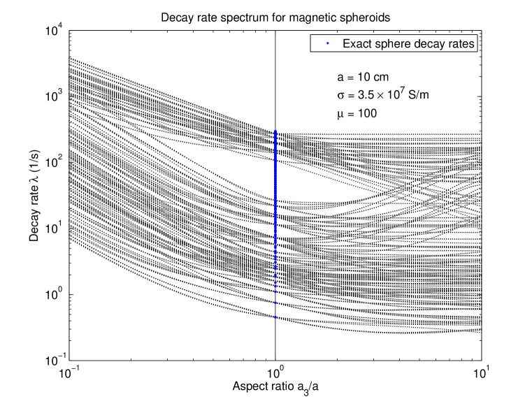
Figure 10: Decay rate spectrum vs. aspect ratio $\alpha=a_{3}/a$ for strongly magnetic/ferrous spheroids ($\mu=100$). All 232 decay rates computed using 232 basis functions each for the electric and magnetic fields with order $N=l+2p\leq 7$ are plotted for 201 values in the range $0.1\leq\alpha\leq 10$. Blue dots at $\alpha=1$ show exact analytic results for the sphere. The corresponding results for nonmagnetic spheroids are shown in Fig. 2. As described in the text, the large value of $\mu$ effectively divides the modes into two sets, one with much higher decay rates. The apparent mode gap near the center of the figure would be filled in with increasing $N$ (as would smaller gaps that contain unmatched sphere modes).

IX.3 Freely decaying mode computation

The freely decaying modes once again correspond to solutions to the homogeneous equations (176) or (185) in which the background terms vanish. Solutions will exist only for special values of the frequency $\omega=-i\lambda$. For nonmagnetic targets (see Sec. II.4) the frequency enters the eigenvalue equation (43) as a trivial multiplier (in the coefficient $Q_{EE}$), and the modes are straightforward solutions to the generalized eigenvalue equation (45).

For magnetic targets the frequency enters the $Q$-parameters (175) in a way that cannot simply be factored out of the $2\times 2$ block operator. Rather, one obtains a form

$$\hat{\cal O}{\bf A}=\hat{\cal H}(\lambda){\bf A}$$ (235)

in which ${\bf A}=({\bf a},{\bf b})^{T}$ and $\hat{\cal O}$, $\hat{\cal H}$ represent the $2\times 2$ operators in (185). Thus, the modes correspond to special values $\lambda_{n}$ in which $\hat{\cal H}(\lambda_{n})$ has a unit (generalized) eigenvalue. To compute these one therefore proceeds as follows. First, solve the generalized eigenvalue problem

$$\hat{\cal O}{\bf A}_{n}(\lambda)=\eta_{n}(\lambda)\hat{\cal H}(\lambda){\bf A}_{n}(\lambda)$$ (236)

for each fixed $\lambda$. The $|\eta_{n}(\lambda)|$ are increasing functions of $\lambda$, and beginning with small $\lambda$, there will be sequence of increasing values $\lambda_{n}$ for which $\eta_{n}(\lambda_{n})=1$ foot:negeval . These are the sought after decay rates, and the corresponding ${\bf A}_{n}(\lambda_{n})$ represent the mode shapes. This search requires on the order of ten repeated diagonalizations to find an individual $\lambda_{n}$, hence thousands to find the entire spectrum. The task is therefore quite numerically intensive (though at least the subblock matrices ${\bf R}$, ${\bf S}$, ${\bf U}$, ${\bf V}$ do not need to be recomputed at each step). Spectra resulting from such a computation, using the ferrous value $\mu=100$, are shown in Fig. 10.

There is an interesting feature in Fig. 10 that deserves comment. Unlike for $\mu=\mu_{b}$ (Fig. 2) where the larger decay rate values are found to progressively fill in as the basis function order $N$ increases, the $\mu/\mu_{b}=100$ case shown in the figure apparently displays two classes of modes that are widely separated in decay rate (at least near the center of the plot). As $N$ increases the gap is expected to gradually fill in (as indicated by the exact sphere results).

The pattern occurs because of the large value of $\mu/\mu_{b}$, and is explained by examining the mode shapes themselves. As discussed in Sec. IX.2, as $\mu/\mu_{b}\to\infty$ the magnetic field boundary normal vanishes, ${\bf H}\cdot{\bf\hat{n}}\to 0$. In fact, this convergence is conditional. For given finite $\mu/\mu_{b}$ there will be more slowly decaying modes for which ${\bf H}\cdot{\bf\hat{n}}=O(\mu_{b}/\mu)$ is indeed small (compared to the transverse component $|{\bf\hat{n}}\times{\bf H}|$), and the decay rate converges to a finite value in the limit $\mu_{b}/\mu\to 0$. However, there are also magnetically polarized modes for which ${\bf H}\cdot{\bf\hat{n}}$ is not small compared to $|{\bf\hat{n}}\times{\bf H}|$ (e.g., for which ${\bf H}$ is fairly uniform inside the target), and these decay much more rapidly. The mode shapes of the higher and lower groups of modes in Fig. 10 indeed exhibit precisely this difference. The interesting non-monotonic behavior of some of the mode curves with increasing aspect ratio probably originates from similar effects (and would go away at high enough order $N$).

It should be noted that this division is directly analogous to the distinct inductive and polarization/non-inductive responses discussed in Secs. I.2 and VII.1 that occur for large conductivity contrast, $\sigma/\sigma_{b}\gg 1$, though the division here is much less extreme because $\mu/\mu_{b}\ll\sigma/\sigma_{b}$ foot:earlyt .

Note, finally, that the reduction/truncation of the magnetic field basis functions described in Sec. IX.2.1 to those with strictly vanishing surface normal eliminates these magnetic polarization modes at the outset. The corresponding off-diagonal reduction (200) of the matrix equation also restores a simple dependence of the decay rates on the spectrum of ${\cal H}$, namely the inverse quadratic relation (212). The approximate validity of this relation can also be used to speed up the previously described $\lambda_{n}$ search for large but finite $\mu/\mu_{b}$.

IX.4 More general target geometries

IX.4.1 Hollow targets

The theory presented here is valid even if $V_{s}$ is not simply connected, or even connected at all. However, the Chandrasekhar theory is specific to solid ellipsoids (Sec. V). Unfortunately, many of the most interesting targets, especially UXO, are hollow (UXO shell thicknesses are in the neighborhood of 10% of the radius). At early time currents reside only near the outer surface of the target and the hollow portion plays no role W2003 ; W2004 . However, at intermediate time and beyond, when the currents penetrate throughout the target, the dynamics is very different. In particular, the leading decay rates scale inversely with the shell thickness (see the upper panel of Fig. 9; analogous also to the scaling with small aspect ratio seen on the left hand side of Fig. 2). The result is a strong deviation from the solid sphere result that begins earlier and earlier as the shell thickness decreases (lower panel of Fig. 9). Accurate modeling in this regime therefore requires extension of the formalism to hollow targets.

There are main two issues. The first is the generalization of the polynomial basis functions described in Sec. II.3.2. The rescaling (34) from the sphere to the ellipsoid works only if the hollow portion is concentric and geometrically similar to the surrounding target, i.e., with axes defined by ${\bf a}_{h}=\alpha_{h}{\bf a}$, $0\geq\alpha_{h}<1$. The underlying $i=1$ sphere basis functions [first line of (II.3.2)] then remain unchanged, while the $i=2$ basis functions are replaced by

$${\bf Z}_{lmp}^{(2)}=\nabla\times[(x^{2}-\alpha_{h}^{2})(1-x^{2})x^{l+2p}{\bf X}_{lm}].$$ (237)

The factor $(x^{2}-\alpha_{h}^{2})(1-x^{2})$ enforces vanishing of the normal component ${\bf Z}_{lmp}^{(2)}$ at both boundaries. The concentric-similar assumption is almost certainly adequate for most UXO.

The second issue is the evaluation of the Coulomb integral matrix elements (31) or (180). Given a polynomial $p({\bf x})$, the basic Coulomb integral may be written as the difference of two solid ellipsoid integrals

$$P({\bf x}) = \hat{\cal K}_{1}[p]({\bf x})$$

$$= \int_{V_{s}({\bf a})}d^{3}x^{\prime}\frac{p({\bf x}^{\prime})}{4\pi|{\bf x}-{\bf x}^{\prime}|}-\int_{V_{s}({\bf a}_{h})}d^{3}x^{\prime}\frac{p({\bf x}^{\prime})}{4\pi|{\bf x}-{\bf x}^{\prime}|}.$$

Both may be evaluated analytically using the methods of Sec. V for arbitrary ${\bf a}_{h}$ (and arbitrary center placement).

The problem is that, since ${\bf x}$ is external to the $V_{s}({\bf a}_{h})$, the second integral is not a polynomial, but a sum of polynomials multiplied by elliptic functions [themselves depending on the nonzero function $\lambda({\bf x})$ defined by (73)]. The second volume integral entering the matrix elements, namely of $P({\bf x})$, or its derivatives, multiplied by a second polynomial, then requires a numerical evaluation. This is not a major barrier to implementing the more general theory, but it does require some extra numerical effort that will be part of future work.

IX.4.2 Multiple targets

The formalism may be also be extended, with a similar level of effort, to multiple targets. The individual target basis functions are unchanged from those of an isolated target. The difficulty again comes from the second volume integral entering the matrix elements: the mutual induction manifests in the integrals such as

$$R_{12}=\int_{V_{s}^{2}}d^{3}xp_{2}({\bf x})\int_{V_{s}^{1}}d^{3}x^{\prime}\frac{p_{1}({\bf x}^{\prime})}{4\pi|{\bf x}-{\bf x}^{\prime}|},$$ (239)

in which the external field in a second target volume $V_{s}^{2}$, generated by a polynomial function $p_{1}$ in the first target volume $V_{s}^{1}$, is integrated against a polynomial function $p_{2}$ in the second target. Once again, even for simple targets where this external field can be expressed in terms of elliptic functions, the second integral requires in general a numerical evaluation. For well separated targets, the mutual induction will be weak, and a local gradient expansion about the center of $V_{s}^{2}$ will provide accurate analytic results. However, for closely spaced, strongly interacting targets, which is the physically more interesting regime, such an approximation will break down.

IX.5 Effects of inhomogeneous background permeability

Beyond the general results (165) and (172), the results presented in this section are specialized to the limit of homogeneous background permeability. The problem is that, unlike background conductivity variations, which do not affect the inductive response as long as the conductivity contrast remains high, even small soil permeability variations (around unity) will impact the induced voltage via the $\mu_{b}$-dependence of the magnetic Green function (163).

The biggest impact is the direct reflection from the ground surface. In the absence of an air-ground permeability contrast the soil is essentially transparent to the low frequency signals considered here. However, even for very small air-ground contrast (say, 1% or less), the direct reflection can mask the signals (which remain essentially unchanged, at the 1% level) from smaller and/or more deeply buried targets. The ground response is much flatter in frequency than that of the target, and so the latter can still be distinguished (though even this assumption can break down if the permeability is frequency-dependent, e.g., if the soil magnetic impurities have nontrivial magnetodynamics). If the background permeability has slow enough spatial variation, the problem can also be ameliorated through a target-absent background subtraction. If the permeability is known and the ground is flat, this subtraction could also be computed theoretically (essentially from the corresponding plane interface Fresnel coefficient). Again, for 1% level accuracy, the target response may be computed assuming homogeneous ground permeability, and simply added to the ground reflection.

For larger permeability contrast, and/or highly variable soils (e.g., strongly magnetic volcanic soils foot:kahoolawe ) the target response becomes much more difficult to discern. Given accurate prior knowledge of $\mu_{b}({\bf x})$, there is no barrier in principle to computing an adequate approximation to the magnetic Green function (163) in the target neighborhood (e.g., as a polynomial-modified Coulomb singularity; analytic forms are also available for horizontally stratified media) and using this to solve for the internal field mode shapes. Intuitively, one expects adjustments in the target current patterns due to mutual induction with neighboring magnetic impurity concentrations. More difficult are the background and external fields, which will experience $\mu_{b}$ over a larger volume and hence require a more comprehensive model to compute.

In conclusion, there appears to be some interesting future work to be performed modeling the basic phenomenology of the effects of magnetically variable backgrounds, but in the presence of high, unpredictable variability foot:kahoolawe , the background subtraction problem has no simple solution—the number of unknown parameters is too large to constrain using limited survey data confined to above-ground measurements.

- (1) See, e.g., J. D. Jackson Classical Electrodynamics (John Wiley and sons, New York, 1975).
- (2) For a related numerical approach using an expansion in spheroidal wavefunctions, see: B. E. Barrowes, K. O’Neill, T. M. Grzegorczyk, X. Chen, and J. A. Kong, IEEE Trans. Geosci. Remote Sens. 42, 2479 (2004); X. Chen, K. O’Neill, T. M. Grzegorczyk, and J. A. Kong, IEEE Trans. on Geosci. Remote Sens. 45, 697 (2007); B. E. Barrowes, K. O’Neill, T. M. Grzegorczyk, B. Zhang, and J. A. Kong, IEEE Trans. Geosci. Remote Sens. 46, 1164, (2008).
- (3) S. Chandrasekhar, Ellipsoidal figures of equilibrium (Dover, 1958).
- (4) P. B. Weichman, Chandrasekhar theory of electromagnetic scattering, arXiv:1108.2239v1 [physics.class-ph].
- (5) Even relatively weak soil permeability (1% or less) can have a very large effect. The air-soil magnetic contrast leads to reflections that can mask the weaker signals from smaller, more deeply buried targets. This becomes an issue, especially, in certain volcanic areas foot:kahoolawe . In Sec. IX.5 we briefly discuss how one may attempt to incorporate such effects into the model, but such an approach can be useful only if the variability is sufficiently predictable and the required magnetostatic model sufficiently simple.
- (6) For a brief review, see P. B. Weichman and E. M. Lavely, Proc. SPIE Vol. 5089 Detection Technologies for Mines and Minelike Targets VIII (SPIE, Bellingham, WA, 2003), p. 1139.
- (7) P. B. Weichman, Phys. Rev. Lett. 91, 143908 (2003).
- (8) P. B. Weichman, Phys. Rev. Lett. 93, 023902 (2004).
- (9) Clearly, for the highly conducting targets of interest, will always dominate , but for very dry soils, or in air, could dominate . However, the background response will still be quasi-static, and it is easily verified that this more general case may be accounted for with the simple replacement in the development of Sec. II.1. This has no effect on the final result, which relies only on the formal limit .
- (10) This is, of course, the same conclusion as would be obtained from the usual condition of continuity of across the bounday in the limit where .
- (11) The matrix would be the identity matrix if the basis functions are additionally orthornormal with respect to the density . However, this is not required and may be inconvenient.
- (12) I. S. Gradshteyn and I. M. Ryzhik, Table of Integrals, Series, and Products (Academic Press, New York, 1981).
- (13) See, e.g., P. M. Morse and H. Feschbach, Methods of Theoretical Physics (McGraw Hill, New York, 1953).
- (14) W. H. Press, B. P. Flannery, S. A. Teukolsky, and W. T. Vetterling, Numerical Recipes, (Cambridge University Press, 1986).
- (15) The integral relation (129) may actually be diagonalized using ellipsoidal harmonics, but the harmonics themselves are very complicated MF , and their computation is not necessarily easier than the matrix inversion route based on the Chandrasekhar approach laid out in Secs. III–V Chandra .
- (16) The non-inductive part may in principle be computed as well using (22). For homogeneous target and background, where the right hand side of (22) is supported on the target boundary, this may be formulated as a Laplace-Neumann problem with boundary values provided by the internal field. However, as discussed in the Introduction, this case is not physically realistic, and is seldom sufficently constrained to enable accurate computation of .
- (17) This is the same estimate as would used to determine the rate of decay of current flowing in circular loop.
- (18) There is an interesting measurement theory sublety inherent in the computation (150)–(159). Both the transmitter and receiver loops are conducting wires whose conductivity should, in principle, be included in the conductivity distribution . Since will again be very large inside the wires, this will have a very large effect on the mode shape in this region, and one may question the use of the unperturbed mode shape in (153) and (154). The decay rate will be perturbed as well, but only in proportion to their mutual inductance as compared to the self inductance of the target, which is very small. The paradox is explained by converting (154) and (159) to the area integrals of the magnetic flux: e.g., , where is the local surface normal. and is the modal magnetic field. Under the reasonable assumption that the self inductance of the wires is very small (which would part of the design specification), the contribution of the immediate wire neighborhood to the area integral is small, and it is therefore dominated by the much larger area over which the perturbed and unperturbed are essentially identical. It follows that the line integral (154) is insensitive to the presence of the transmitter wire, even though the local values of are highly sensitive. For any type of measurement, there is always a calibration that must be performed to relate the device output to the local values of the unperturbed fields in the absence of the measurement apparatus. In this case the procedure is relatively straightforward.
- (19) Another technical issue that must be addressed in any comparison with data is that modes are computed in the natural frame of the target principle axes, whereas measurements are performed in the laboratory frame, in which both the measurement apparatus and the target may have some nontrivial orientation. The electric field computations are most conveniently performed in the natural frame, so once a lab frame evaluation point is determined from the placement of transmitter and receiver loops [which also specifies the lab frame orientation of line integral increments in (154) and (159)], the lab frame electric field is expressed as . Here is the usual rotation matrix that converts the components of a vector in the natural frame to those in the lab frame via .
- (20) For larger targets, for lower order modes be much larger (100 ms or more) than the interval between periodic pulses (typically tens of ms), and the integral (155) will encompass several pulses. A typical measurement averages over many pulses, and the resulting is a geometric series that may still be summed analytically.
- (21) Applications of the present theory to target inversion problems, where, for example, multi-sensor data providing multiple “looks” at the target is extremely useful, lies beyond the scope of the present article, and will be presented elsewhere.
- (22) The TEMTADS platform, besides its use for scientific data collection, is designed to be towed behind a vehicle (hence the full name, Time-domain Electro-Magnetic Towed Array Detection System) and is actively used for UXO remediation work in this configuration. See, e.g., G. R. Harbaugh, D. A. Steinhurst, D. C. George, J. B. Kingdon, D. K. Keiswetter, and T. H. Bell, “EMI Array for Cued UXO Discrimination” at http://serdp-estcp.org/.
- (23) The transmitter coil windings are actually spread out over 7.8 cm in height. However, modeling them as 1D ideal loops centered at 3.9 cm above their base suffices for targets at reasonable standoff (say, centered 20 cm or more below the plane of the loop). The receiver coils are compact in height, and lie at the bases of the transmitter coils, so their centers lie 3.9 cm below the effective center of the latter. Due to the rapid decay of the signals with target depth, these details turn out to be quantitatively important: prior to incorporating them, the comparisons in Fig. 7 contained 10–20% systematic biases that could not be explained by any known measurement uncertainty (e.g., the known pulse amplitude variability cited in the caption to Fig. 7) or calibration error.
- (24) Since one actually knows that , one could use the more restricted set of basis functions at the outset. However, it is found that better numerical stability is obtained by letting the equations themselves impose this identity on the solution.
- (25) One typically finds that for slowest decay rate one has , which yields . thus is actually an order of magnitude larger than the fundamental decay rate. Thus, according to (193), for , one will need for the term to dominate.
- (26) If one integrates over some surface the result is the monopole flux through that surface. Using Ampere’s law, the same result is obtain by integrating the tangential component of around the contour enclosing . The form (213) may then be derived by taking to be the circle at fixed polar angle , which then equates to the enclosed flux .
- (27) This follows very generally from the formal observation that the parity operator commutes with , irrespective of the value of . Therefore the eigenvectors may always be chosen to have definite parity.
- (28) In fact, only half the actually cross unity. The other half remain negative for all and correspond to unphysical solutions for which the Maxwell relation fails. This explains how the doubling of the matrix size, in which (172) is used together with (165) instead of enforcing the Maxwell relation at the outset by substituting it directly into (165), does not lead to a doubling of the number of modes. This structure can be verified explicitly in the exact solution of the sphere, where the come in equal but oppositely signed pairs.
- (29) It is the existence of these magnetic polarization modes for large but finite that also leads to the crossover at very early time from the magnetic target characteristic time-domain voltage power law back to the non-magnetic power law W2004 .
- (30) A well known example in the UXO remediation community is the former Navy test range on the island of Kaho’olawe, Hawaii (see, e.g., http://en.wikipedia.org/wiki/Kahoolawe).