Evidence of non-mean-field-like low-temperature behavior in the Edwards-Anderson spin-glass model

Abstract

The three-dimensional Edwards-Anderson and mean-field Sherrington-Kirkpatrick Ising spin glasses are studied via large-scale Monte Carlo simulations at low temperatures, deep within the spin-glass phase. Performing a careful statistical analysis of several thousand independent disorder realizations and using an observable that detects peaks in the overlap distribution, we show that the Sherrington-Kirkpatrick and Edwards-Anderson models have a distinctly different low-temperature behavior. The structure of the spin-glass overlap distribution for the Edwards-Anderson model suggests that its low-temperature phase has only a single pair of pure states.

Spin glasses Binder and Young (1986) have been the subject of intense study and controversy for decades. These models are perhaps the simplest, physically-motivated examples of frustrated systems in classical statistical mechanics. Given their wide applicability across disciplines, it is important that their behavior is understood. Despite four decades of research, the low-temperature phase of short-range spin glasses is poorly understood. Here we study both the three-dimensional (3D) Edwards-Anderson (EA) Ising spin glass Edwards and Anderson (1975) and the Ising spin glass on a complete graph—known as the Sherrington-Kirkpatrick (SK) model Sherrington and Kirkpatrick (1975)—in an effort to gain a deeper understanding of the low-temperature spin-glass state. Our results suggest that these models are qualitatively different at low temperatures.

Parisi’s solution of the SK model Parisi (1979, 1983) involves an unusual form of symmetry breaking among replicas. These were originally introduced to carry out the disorder average of the logarithm of the partition function. The low-temperature phase of the model within the replica symmetry breaking (RSB) solution Parisi (1979, 1983) has several unusual features such as the breakdown of self-averaging and the co-existence of a countable infinity of pure states in the thermodynamic limit.

Figure 1: (Color online) (a) In the droplet picture $P(q)$ is trivial with one pair of pure states. (b) In the RSB picture individual samples have many pairs of pure states ($\delta$ functions in $P_{\cal J}(q)$). (c) In the RSB picture $P(q)$ is nontrivial (continuous support for $|q|<q_{\rm EA}$).

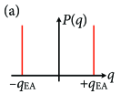
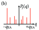
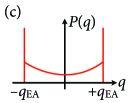
There is no analytic theory for the EA model but it is well-accepted on the basis of numerical simulations Katzgraber et al. (2006) that the EA model undergoes a continuous phase transition. However, the low-temperature broken-symmetry phase is not understood, even qualitatively. Different mutually-exclusive scenarios have been proposed: The replica symmetry breaking (RSB) picture is based on an analogy with the solution of the SK model. It assumes that self-averaging breaks down and that there are a countable infinity of pure states in the thermodynamic limit. A qualitatively different and simpler picture was proposed to describe the EA model by McMillan, Fisher and Huse, as well as Bray and Moore McMillan (1984); Fisher and Huse (1986, 1987, 1988); Bray and Moore (1986). In the “droplet scaling” picture the low-temperature phase is described by one pair of pure states related by a spin flip with low-lying excitations that are isolated, compact droplets of the opposite phase. A central difference between the RSB and droplet pictures for the EA model is whether there is a single pair of pure states or many pairs of pure states for large systems, see Fig. 1.

Newman and Stein Newman and Stein (1992, 1996, 1998) explained that the usual way of constructing the thermodynamic limit cannot be applied to finite-dimensional spin glasses because of the possibility of a chaotic system-size dependence in which different thermodynamic states may appear for different system sizes. They showed that the key ideas of RSB—non-self-averaging and a countable infinity of pure states—cannot hold for the EA model within the naïve way that they were first proposed. However, their results do not completely rule out a nonstandard interpretation of RSB. They also proposed a more plausible many-states “chaotic pairs” picture in which for a fixed choice of couplings, there are many pure states but that in a single finite volume only one pair is manifest.

Here we report the results of large-scale Monte Carlo simulations of both the SK and EA models. Our objective is to shed light on the qualitative nature of the low-temperature phase of the EA model by comparing and contrasting to the SK model. Previous numerical studies, e.g., Katzgraber et al. (2001) using the average spin overlap distribution suggested that both the SK and EA models are well described by the RSB picture. However, for the numerically-accessible system sizes the two main peaks are still converging to $\pm q_{\rm EA}$ (see Fig. 3) and therefore results might be plagued by finite-size effects. On the other hand, studies of the link overlap Katzgraber et al. (2001) distribution suggest agreement with the droplet picture. The “trivial nontrivial” scenario Palassini and Young (1999); Krzakala and Martin (2000); Katzgraber et al. (2001) reconciles these numerical results by postulating that excitations are compact, as in the droplet picture, but their energy cost is independent of system size, as in the RSB picture. In an effort to resolve these discrepancies, here we introduce a statistic obtained from the spin overlap distribution that detects sharp peaks in individual samples, inspired by a recent study on the SK model Aspelmeier et al. (2008). This statistic clearly differentiates the RSB and droplet pictures: it converges to zero in the large-volume limit if there is a single pair of pure states and to unity if there are countably many. Our results for this quantity shows clear differences between the EA and SK models.

Models and Numerical Details.—

The SK and EA models are defined by the Hamiltonian ${\mathcal{H}}=-\sum_{i,j=1}^{N}J_{ij}S_{i}S_{j}$, with $S_{i}\in\{\pm 1\}$ Ising spins. For the EA model the sum is over nearest neighbors on a cubic lattice of size $N=L^{3}$ with periodic boundaries. The couplings $J_{ij}$ are chosen from a Gaussian distribution with zero mean and variance unity. A set of couplings ${\cal J}=\{J_{ij}\}$ defines a disorder realization or, simply, a “sample.” For the SK model the sum is over all pairs of spins and the $J_{ij}$ are chosen from a Gaussian distribution with zero mean and variance $1/(N-1)$.

Ordering in spin glasses is detected from the spin overlap $q=(1/N)\sum_{i}S^{\alpha}_{i}S^{\beta}_{i}$, where “$\alpha$” and “$\beta$” indicate independent spin configurations for the same sample ${\cal J}$. The primary observable we consider for fixed ${\cal J}$ and $N$ is the overlap probability density, $P_{\cal J}(q)$. In the high-temperature phase there is a well-defined thermodynamic limit and $P_{\cal J}(q)\to\delta(q)$ for $N\to\infty$ for almost every ${\cal J}$. The behavior of $P_{\cal J}(q)$ for large $N$ and $T<T_{c}$, $T_{c}$ the critical temperature, distinguishes the RSB picture from other theories. If there is only a single pair of states for each system size, $P_{\cal J}(q)$ consists for large $N$ of a symmetric pair of $\delta$ functions at the Edwards-Anderson order parameter $q=\pm q_{\rm EA}$, see Fig. 1. In the RSB picture there are many sharp peaks symmetrically distributed in the range $-q_{\rm EA}<q<q_{\rm EA}$ as shown in Fig. 1, corresponding to multiple pairs of pure states. In the RSB picture, the distribution of peaks depends on ${\cal J}$ but the disorder averaged overlap distribution $P(q)$ exists, and for large $N$ is expected take the form shown in Fig. 1.

We have carried out replica exchange Monte Carlo Hukushima and Nemoto (1996) simulations of both models. Parameters are shown in Tables 1 and 2. For each sample we equilibrate two independent sets of replicas to compute the overlap distribution. Equilibration is tested for the EA and SK models using the methods of Refs.Katzgraber et al. (2001) and Hukushima et al. (1998), respectively. The number of equilibration and data collection sweeps are chosen to be long enough to ensure that samples are well equilibrated and that $P_{\cal J}(q)$ is accurately measured for each sample. We report results for $T=0.42$ [$T=0.4231$] for the EA [SK] model. For the EA model, $T_{c}\approx 0.96$ Katzgraber et al. (2006), while for the SK model $T_{c}=1$, so our simulations are at $\sim 0.4T_{c}$, i.e., deep within the spin-glass phase com (a) where critical fluctuations are unimportant.

Table 1: EA model simulation parameters. For each number of spins $N=L^{3}$ we equilibrate and measure for $2^{b}$ Monte Carlo sweeps. $T_{\rm min}$ [$T_{\rm max}$] is the lowest [highest] temperature and $N_{T}$ is the number of temperatures. $N_{\rm sa}$ is the number of disorder samples.

$N$	$L$	$b$	$T_{\rm min}$	$T_{\rm max}$	$N_{T}$	$N_{\rm sa}$
$64$	$4$	$18$	$0.2000$	$2.0000$	$16$	$4891$
$216$	$6$	$24$	$0.2000$	$2.0000$	$16$	$4961$
$512$	$8$	$27$	$0.2000$	$2.0000$	$16$	$5130$
$1000$	$10$	$27$	$0.2000$	$2.0000$	$16$	$5027$
$1728$	$12$	$25$	$0.4200$	$1.8000$	$26$	$3257$

Table 2: Simulation parameters for the SK spin glass. See the Table 1 for details.

$N$	$b$	$T_{\rm min}$	$T_{\rm max}$	$N_{T}$	$N_{\rm sa}$
$64$	$22$	$0.2000$	$1.5000$	$48$	$5068$
$128$	$22$	$0.2000$	$1.5000$	$48$	$5302$
$256$	$22$	$0.2000$	$1.5000$	$48$	$5085$
$512$	$18$	$0.2000$	$1.5000$	$48$	$4989$
$1024$	$18$	$0.2000$	$1.5000$	$48$	$3054$
$2048$	$16$	$0.4231$	$1.5000$	$34$	$3020$

Results.—

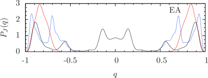
Figure 2 shows $P_{\cal J}(q)$ for three different EA samples ($N=512=8^{3}$, $T=0.42$). Note that $P_{\cal J}(q)$ varies considerably between samples. Qualitatively similar overlap distributions are seen for the SK model. Figure 3, left panel [right panel], shows the disorder averaged overlap distribution $P(q)$ for the EA [SK] model for different system sizes at $T=0.42$ [$T=0.4231$] com (b). At this low temperature, $P(q)$ consists of large peaks at the finite-size value of the EA order parameter, $\pm q_{\rm EA}(N)$. $P(q)$ is reasonably flat, non-zero, and nearly independent of $N$ in the approximate range $-0.4\lesssim q\lesssim 0.4$ for the sizes studied here. We can quantify this observation by considering the integrated overlap, $I(q_{0})=\int_{|q|<q_{0}}P(q)dq$. Figure 4 shows $I(0.2)$ as a function of $N$ for both the EA and SK models at $T\approx 0.4T_{c}$ com (a). Note that $I(0.2)$ is nearly independent of $N$. We found qualitatively similar results for other values of $q_{0}$ up to $q_{0}\approx 0.5$ and temperatures down to $0.2T_{c}$ for smaller systems. The constancy of $I(0.2)$ has been observed in a number of studies (see Refs. Katzgraber et al. (2001) and Alvarez Baños et al. (2010)) and is among the strongest evidence in favor of the validity of the RSB picture for short-range systems.

Figure 2: (Color online) Typical overlap distributions $P_{\cal J}(q)$ for three disorder realizations for the EA model with $N=8^{3}$ and $T=0.42$.

Figure 3: (Color online) Disorder-averaged overlap probability distribution $P(q)$ for different system sizes at $T=0.42$ and $T=0.4231$ for the EA model (left) and SK model (right), respectively.

Figure 4: (Color online) Disorder average of the weight of the overlap distribution $I(0.2)$ as a function of $N$ for $T\approx 0.4T_{c}$ for both the EA and SK models.

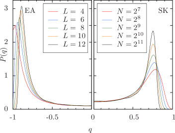
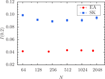
Although $I(q_{0})$ in Fig. 4 is nearly constant over the range of sizes simulated in this and other studies of the EA model, it is also clear that, for these same sizes there are strong finite-size effects. These corrections can be seen by looking at the size dependence of $q_{\rm EA}(N)$. The peak moves to smaller values of $q_{\rm EA}$ as $N$ increases, similar to recent results Alvarez Baños et al. (2010) for larger $N$. The presence of these strong finite-size corrections makes the absence of any significant $N$ dependence of $P(q)$ for small $q$ surprising. In the droplet picture, $I(q_{0})$ is expected to decay with a small power of $L$, $I(q_{0})\sim TL^{-\theta}$ ($\theta\approx 0.2$ in 3D Hartmann (1999)) and this slow asymptotic behavior may not set in until large sizes. Thus the behavior of $I(q_{0})$ shown in Fig. 4 may not be a sensitive indicator of the nature of the low-temperature phase for system sizes currently accessible to simulation.

To better understand the size dependence of the overlap distributions, we go beyond disorder averages and consider other statistics obtained from $P_{\cal J}(q)$. In particular, we identify the emergence, or not, of $\delta$ functions in the range $-q_{\rm EA}<q<q_{\rm EA}$ as $N$ increases, which would signal more than one pair of pure states. A finite-size broadened $\delta$ function at $q$ is characterized by a large value of $P_{\cal J}(q)$. To detect $\delta$-function-like behavior for finite $N$ we consider the statistic

$$\Delta(q_{0},\kappa)={\rm Prob}\left[\max_{|q|<q_{0}}\bigg{\{}\frac{1}{2}\big{(}P_{\cal J}(q)+P_{\cal J}(-q)\big{)}\bigg{\}}>\kappa\right].$$ (1)

The probability is defined with respect to ${\cal J}$ and $\Delta(q_{0},\kappa)$ is the fraction of samples with at least one peak greater than $\kappa$ in $P_{\cal J}(q)$ in the range $|q|<q_{0}$. $\kappa$ is chosen to be large enough to exclude some but not all samples. We refer to samples counted in $\Delta(q_{0},\kappa)$ as “peaked.” For example, with $\kappa=1$ the sample with the central peaks (black line) in Fig. 2 is peaked for $q_{0}\gtrsim 0.1$, whereas the two other samples are not for $q_{0}\lesssim 0.5$.

The droplet and RSB pictures make dramatically different predictions for $\Delta(q_{0},\kappa)$. For the droplet or chaotic pairs picture there is only a single pair of states for any large volume so that $\Delta(q_{0},\kappa)\to 0$ for any $\kappa>0$ and any $q_{0}<q_{\rm EA}$ when $N\to\infty$. However, for the RSB picture one expects $\delta$ functions in $P_{\cal J}(q)$ for any range of $q$, i.e., $\Delta(q_{0},\kappa)\to 1$ as $N\to\infty$ for any $q_{0}$ and $\kappa>0$.

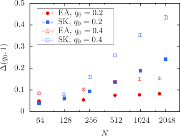
Figure 5 shows $\Delta(q_{0},\kappa)$ as a function of system size for $q_{0}=0.2$ and $0.4$, as well as $\kappa=1$ com (c). We found qualitatively similar results for other values of $q_{0}$ and $\kappa$, as well as for lower temperatures. Our most important observation is that the fraction of peaked samples $\Delta(q_{0},\kappa)$ is nearly constant and small for the EA model while $\Delta(q_{0},\kappa)$ is increasing over the same range of $N$ for the SK model com (d). The result for the SK model is expected from Parisi’s RSB solution. The contrasting result for the EA model suggests that the number of pure states does not grow with the system size for low $T$; a result consistent with the droplet and chaotic pairs pictures.

Figure 5: (Color online) Fraction of peaked samples $\Delta(q_{0},\kappa)$ at $T\approx 0.4T_{c}$ as a function of $N$ for $\kappa=1$, $q_{0}=0.2$ and $0.4$.

Figure 6: (Color online) Contours of constant $\Delta$ for the EA model (left) and the SK model (right) as a function of $\log_{10}(N)$ and $\log_{10}(\kappa/\kappa_{0})$ with $\kappa_{0}=0.5$ and $1.5$ for $q_{0}=0.2$ and $1.0$, respectively. The solid [dashed] lines are contours of constant $\Delta$ for $q_{0}=0.2$ [$q_{0}=1.0$] equally spaced in $\Delta$ com (e).

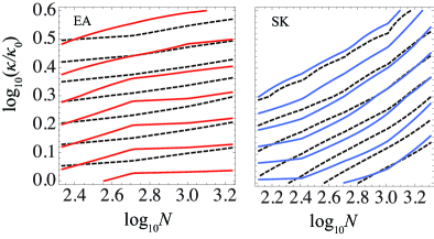
The difference in the behavior of $\Delta$ for the SK model in comparison to the EA model might be explained by the fact that peaks sharpen more quickly with $N$ for the SK than for the EA model (see Fig. 3 and Ref. Fernández and Alonso (2012). To study this effect, we compare $\Delta$ for the two values, $q_{0}=0.2$ and $q_{0}=1$, for each model separately. For $q_{0}=1$, $\Delta$ is controlled by the peaks at $\pm q_{\rm EA}$ and must converge to unity for both models because for $N\rightarrow\infty$ the $q_{\rm EA}$ peaks become $\delta$ functions. Figure 6, left [right] panel, shows contour plots of constant $\Delta$ for the EA [SK] model. The horizontal axis is the logarithm of the number of spins and the vertical axis is the logarithm of $\kappa/\kappa_{0}$ with $\kappa_{0}=0.5$ for $q_{0}=0.2$ and $\kappa_{0}=1.5$ for $q_{0}=1$. The curves are lines of constant $\Delta$ obtained from a linear interpolation of the data. Each set of curves are equally spaced in $\Delta$ com (e) with $\Delta$ decreasing as $\kappa$ increases. The dashed contours are for $q_{0}=1$ and thus include the $q_{\rm EA}$ peaks. As expected, the dashed contours are clearly increasing functions for both models although they rise more rapidly for the SK model than for the EA model. The solid curves are contours of constant $\Delta$ for $q_{0}=0.2$. Close inspection of the data reveals a qualitative difference between both models. For large $N$ and large $\Delta$, the SK $q_{0}=0.2$ contours rise more steeply than the corresponding $q_{0}=1$ contours, suggesting that not only are peaks sharpening, but the number of peaks is also increasing. In fact, Ref. Aspelmeier et al. (2008) shows that the number of peaks in $P_{J}(q)$ should scale as $N^{1/6}$ for the SK model. On the other hand, for large $N$ and large $\Delta$, the EA contours for $q_{0}=0.2$ are nearly flat, rising less steeply than for $q_{0}=1$, suggesting that the number of peaks is either decreasing or staying constant.

Conclusions.—

We introduce a statistic $\Delta$ that detects the fraction of samples with $\delta$ function behavior in $P_{\cal J}(q)$ near the origin and sharply distinguishes the RSB picture from scenarios with only a single pair of states such as the droplet picture. While our results for the SK model are consistent with RSB, as expected, the EA model does not display a trend towards many pairs of pure states. These results lend weight to the droplet and chaotic pairs pictures It is also possible that for the EA model, $\Delta$ increases very slowly in $N$ and ultimately converges to unity in agreement with the RSB picture. However, our data show no indication of such trend. It would be interesting to perform a similar analysis with extremely large data sets computed with special-purpose computers, such as the Janus machine Belletti et al. (2008).

We thank J. C. Andresen, R. S. Andrist, D. Fisher, D. Huse, E. Marinari, M. Moore, C. Newman, G. Parisi, and D. Stein for useful discussions. H.G.K. acknowledges support from the SNF (Grant No. PP002-114713) and the NSF (Grant No. DMR-1151387). J.M. and B.Y. are supported in part by the NSF (Grant No. DMR-0907235). We thank the Texas Advanced Computing Center, ETH Zurich, and Texas A&M University for providing HPC resources.

References

- Binder and Young (1986) K. Binder and A. P. Young, Rev. Mod. Phys. 58, 801 (1986).
- Edwards and Anderson (1975) S. F. Edwards and P. W. Anderson, J. Phys. F: Met. Phys. 5, 965 (1975).
- Sherrington and Kirkpatrick (1975) D. Sherrington and S. Kirkpatrick, Phys. Rev. Lett. 35, 1792 (1975).
- Parisi (1979) G. Parisi, Phys. Rev. Lett. 43, 1754 (1979).
- Parisi (1983) G. Parisi, Phys. Rev. Lett. 50, 1946 (1983).
- Katzgraber et al. (2006) H. G. Katzgraber, M. Körner, and A. P. Young, Phys. Rev. B 73, 224432 (2006).
- McMillan (1984) W. L. McMillan, Phys. Rev. B 29, 4026 (1984).
- Fisher and Huse (1986) D. S. Fisher and D. A. Huse, Phys. Rev. Lett. 56, 1601 (1986).
- Fisher and Huse (1987) D. S. Fisher and D. A. Huse, J. Phys. A 20, L1005 (1987).
- Fisher and Huse (1988) D. S. Fisher and D. A. Huse, Phys. Rev. B 38, 386 (1988).
- Bray and Moore (1986) A. J. Bray and M. A. Moore, in Heidelberg Colloquium on Glassy Dynamics and Optimization, edited by L. Van Hemmen and I. Morgenstern (Springer, New York, 1986), p. 121.
- Newman and Stein (1992) C. M. Newman and D. L. Stein, Phys. Rev. B 46, 973 (1992).
- Newman and Stein (1996) C. M. Newman and D. L. Stein, Phys. Rev. Lett. 76, 515 (1996).
- Newman and Stein (1998) C. M. Newman and D. L. Stein, Phys. Rev. E 57, 1356 (1998).
- Katzgraber et al. (2001) H. G. Katzgraber, M. Palassini, and A. P. Young, Phys. Rev. B 63, 184422 (2001).
- Palassini and Young (1999) M. Palassini and A. P. Young, Phys. Rev. Lett. 83, 5126 (1999).
- Krzakala and Martin (2000) F. Krzakala and O. C. Martin, Phys. Rev. Lett. 85, 3013 (2000).
- Aspelmeier et al. (2008) T. Aspelmeier, A. Billoire, E. Marinari, and M. A. Moore, J. Phys. A: Math. Theor. 41, 324008 (2008).
- Hukushima and Nemoto (1996) K. Hukushima and K. Nemoto, J. Phys. Soc. Jpn. 65, 1604 (1996).
- Hukushima et al. (1998) K. Hukushima, H. Takayama, and H. Yoshino, J. Phys. Soc. Jpn. 67, 12 (1998).
- com (a) Tests at low give qualitatively similar results.
- com (b) Because is an even function, we show one side of for each model.
- Alvarez Baños et al. (2010) R. Alvarez Baños, A. Cruz, L. A. Fernandez, A. Gordillo-Guerrero, J. M. Gil-Narvion, M. Guidetti, A. Maiorano, F. Mantovani, E. Marinari, V. Martin-Mayor, et al., J. Stat. Mech. P05002 (2010).
- Hartmann (1999) A. K. Hartmann, Phys. Rev. E 59, 84 (1999).
- com (c) The error bars in Fig. 5 are one standard deviation statistical errors due to the finite number of samples. There are also errors due to the finite length of the data collection. To estimate these errors we measured and , defined as in Eq. (1) but from the and components of , respectively. These are expected to be reasonably independent and their differences provide an estimate of the error due to finite run lengths. For all sizes, the average absolute difference between these quantities, is less than the statistical error.
- com (d) Similar results for the SK model were obtained in Ref. Aspelmeier et al. (2008) by counting individual peaks.
- com (e) For the EA model the ranges are for and for . For the SK model the ranges are for and for .
- Fernández and Alonso (2012) J. F. Fernández and J. J. Alonso (2012), (arXiv:cond-mat/1207.4008).
- Belletti et al. (2008) F. Belletti, M. Cotallo, A. Cruz, L. A. Fernández, A. Gordillo, A. Maiorano, F. Mantovani, E. Marinari, V. Martín-Mayor, A. Muñoz-Sudupe, et al., Comp. Phys. Comm. 178, 208 (2008).
- Aspelmeier et al. (2008) T. Aspelmeier et al., J. Phys. A: Math. Theor. 41, 324008 (2008).