Enhanced charge detection of spin qubit readout via an intermediate state

Abstract

We employ an intermediate excited charge state of a lateral quantum dot device to increase the charge detection contrast during the qubit state readout procedure, allowing us to increase the visibility of coherent qubit oscillations. This approach amplifies the coherent oscillation magnitude but has no effect on the detector noise resulting in an increase in the signal to noise ratio. In this letter we apply this scheme to demonstrate a significant enhancement of the fringe contrast of coherent Landau-Zener-St$\ddot{u}$ckleberg oscillations between singlet S and triplet $\text{T}_{\text{+}}$ two-spin states.

The crucial step of spin qubit readout via spin to charge conversion is usually achieved through charge detection technology.Field1993 The maximum sensitivity is related to the difference (contrast) in the charge detection signal of the two charge state configurations. In this letter we demonstrate how this contrast can be amplified by a significant factor if a “state discriminating” relaxation process is introduced during the readout procedure. Since this modification only changes the charge detector contrast between the relevant qubit states, the signal to noise ratio is likewise enhanced.

Spin qubits based on single, double or triple quantum dot circuits have been successfully demonstrated.Petta2005 ; Petta2010 ; Gaudreau2011 Following a coherent manipulation experiment the measurement is usually completed by reading out the final quantum state using a charge detector which is able to distinguish between the quantum spin states.

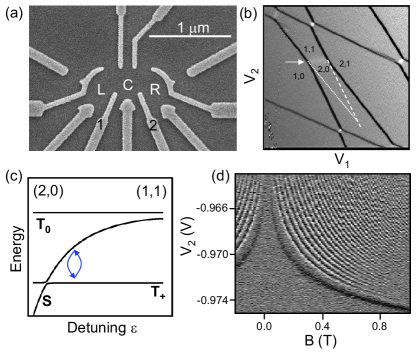
Figure 1: (a) SEM of triple dot structure. (b) Stability diagram as a function of voltages on gates 1 and 2. The charge transfer line between charge states (2,0) and (1,1) is indicated by the arrow. (c) Double dot energy level diagram for dots L and C with dot R acting as a spectator. (d) Typical spin funnel and coherent LZS oscillations observed with the enhanced charge detection technique as a function of initial gate detuning and magnetic field B.

We will concentrate on the qubit based on the singlet (S) and triplet ($\text{T}_{\text{+}}$) two-spin states recently demonstrated by Petta et al.Petta2010 The corresponding oscillations are called Landau-Zener-St$\ddot{u}$ckleberg (LZS) oscillations and are observed as fringes in the stability diagram or when plotted as a function of pulse duration, magnetic field or initial gate detuning. We stress that a similar readout advantage can be implemented for other spin qubit species. The experiments were made using a triple quantum dot device (see Fig. 1(a)).Gaudreau2011 ; Gaudreau2009 ; Granger2010 During our measurements one quantum dot (R) was not coupled via exchange or tunnelling to the other two quantum dots making this effectively a two quantum dot experiment.Studenikin2012 As a result we will use double quantum dot notation throughout. A schematic energy level diagram vs detuning is shown for a double dot in a magnetic field in Fig. 1(c). The two qubit states S and $\text{T}_{\text{+}}$ which differ in spin are coupled via the hyperfine interaction which creates an anticrossing in the energy level diagram.

A generic S/$\text{T}_{\text{+}}$ spin qubit operation for this system would proceed as follows. The quantum state preparation is first achieved by applying a pulse (in reality a combined pulse on gates 1 and 2) from the S(2,0) regime through the anticrossing to the (1,1) charge regime (where ($n_{L}$, $\mbox{$n_{C}$})$ indicate the number of electrons, $n_{L}$ ($n_{C}$) in quantum dots L (C)). A suitable pulse rise time permits a superposition of the S and $\text{T}_{\text{+}}$ states to be generated via Landau-Zener tunnelling on passage through the anticrossing (in an ideal situation this would move the state vector to the equator of the S/$\text{T}_{\text{+}}$ Bloch sphere).Petta2010 Having created the superposition any required manipulation is performed in the (1,1) ground state regime. In this regime and away from the anticrossing, rotations around the Z axis of the Bloch sphere (phase accumulation during the time spent by the pulse beyond the S/$\text{T}_{\text{+}}$ anticrossing) occur with a rate dependent on the energy level spacing (illustrated by arrows in Fig. 1(c)). As can be seen in Fig. 1(c) this depends on the distance from the anticrossing. The final “readout” process takes advantage of the Pauli Blockade phenomenon. The system is moved back to the (2,0) ground state regime where the $\text{T}_{\text{+}}$(1,1) state can only relax to S(2,0) with a relaxation time $\text{T}_{\text{1}}$ ($\sim$100 $\mu$s in these experiments) and coherent behaviour can be measured if $\mbox{$\text{T}_{\text{1}}$}>\mbox{$\text{T}_{\text{m}}$}$, the measurement time ($\sim$10 $\mu$s). The quantum dot circuit state is typically probed by measuring the current through a nearby quantum point contact (QPC) charge detectorField1993 or, occasionally, a neighbouring quantum dot.Barthel2009 The QPC is tuned to be highly sensitivity to local electrostatic conditions (usually at a QPC conductance $<G_{0}=2e^{2}/h$). The (1,1) and (2,0) charge configurations possess different electron distributions and, therefore, have different electrostatic coupling to the charge detector. These can be characterized by I(2,0) and I(1,1) where I is the current through the charge detector for a fixed applied bias. Thus the probability of the occupation of the (2,0) state P(S) oscillates according to the phase accumulation during the pulse and can be measured with a maximum sensitivity contrast equal to I(2,0) - I(1,1). To extract quantitative values for the probability is a complex procedure taking into account $\text{T}_{\text{1}}$ processes during measurement and initialization steps. This is beyond the scope of this letter.

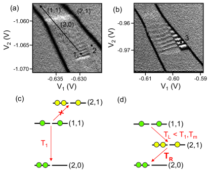
Figure 2: (a) Expanded stability diagram showing LZS oscillations in the the charge detector current taken under conditions in which amplification is suppressed. $T_{R}\sim$10ns, $\text{T}_{\text{m}}$=$4~{}\mu$s, B=100mT, pulse amplitude ($\delta$$\text{V}_{\text{1}}$,$\delta$$\text{V}_{\text{2}}$) = (-8.5,10.0)mV, rise time = 4 ns, duration = 10 ns. Arrow indicates typical voltage pulse. (b) Same as (a) but taken under enhancement conditions. $T_{R}\sim 450\mu$s, $\text{T}_{\text{m}}$=$20~{}\mu$s, B=200mT, pulse amplitude ($\delta$$\text{V}_{\text{1}}$,$\delta$$\text{V}_{\text{2}}$) = (-16.2,20.0)mV, rise time = 3 ns, duration = 7 ns. (c) Schematic energy diagram for unamplified measurement inside triangular part of (2,0) charge region (see Fig. 1(b)) and corresponding to point 1 in (a). (d) Schematic energy diagram for points 2 in (a), 3 in (b) to the right of the triangular region. Enhancement occurs if $T_{L}<\mbox{$\text{T}_{\text{1}}$},T_{R}\geq\mbox{$\text{T}_{\text{m}}$}$.

Consider now the role of excited states in the readout measurement. The $\text{T}_{\text{+}}$(1,1) configuration is an excited state configuration in the (2,0) region (see Fig. 1(b)). The dotted and dashed lines in Fig. 1(b) mark the boundary along which two excited states cross. To the left (right) of the dotted (dashed) line the (1,0) ((2,1)) excited state has a lower energy than the (1,1) excited state. In both cases it is usually observed that the relaxation time from (1,1) to (2,0) is very rapid in these regions mediated first by relaxation to excited states and then by adding (removing) an electron to (from) the spin unpolarized leads i.e. (1,1)$\rightarrow$(1,0)$\rightarrow$(2,0) or (1,1)$\rightarrow$(2,1)$\rightarrow$(2,0). The latter process is illustrated in Fig. 2(d)). These processes usually involve rapid communication with the leads and this typically restricts the useful readout region to the triangle marked in Fig. 1(b) where $\text{T}_{\text{1}}$ can be made larger than the measurement time required for a reasonable measurement visibility.Johnson2005 This is illustrated in Fig. 2(c) for a typical pulse measured within the triangle (point 1 in Fig. 2(a)). Typical LZS fringes obtained using this conventional scheme are shown in Fig. 3(a,c,e).

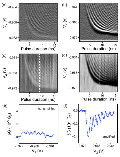
Figure 3: (a)[(b)] Derivative of the QPC conductance with respect to initial detuning component along $\text{V}_{\text{2}}$ as a function of pulse duration and initial detuning for a pulse starting in the unamplified[amplified] region of Fig. 2(b). (c,d) Raw QPC conductances corresponding to (a,b). (e,f) Fixed pulse duration (9 ns) line scans taken from (c,d).

Here we suggest and demonstrate an alternative approach taking advantage of the properties of these metastable states. This scheme leads to dramatically enhanced LZS fringe visibility, an example of which is shown in Fig. 1(d). Typically about 50 coherent oscillations can be observed with this scheme. We focus on modifying the usual $\text{T}_{\text{1}}$ decay path from the (1,1) to (2,0) state. In particular we focus on the (1,1)$\rightarrow$(2,1)$\rightarrow$(2,0) process (the (1,1)$\rightarrow$(1,0)$\rightarrow$(2,0) side of the triangle also shows amplification effects under appropriate conditions and is not discussed further here). A rapid relaxation rate via this path requires an electron of the appropriate spin to enter dot L rapidly (tunneling time $T_{L}$, typically $\sim$0.3 $\mu$s) from the left lead via the process (1,1)$\rightarrow$(2,1) and then for the electron in dot C to exit to the right lead (with tunneling time $T_{R}$) via the process (2,1)$\rightarrow$(2,0) as illustrated for a measurement at point 2 in Fig. 2(a), where $T_{R}\sim 10ns$, in the schematic Fig. 2(d). Consider the consequences of slowing the second process down (a condition which can be trivially accomplished by reducing the coupling to the right lead during the measurement step of the pulse sequence i.e. making $T_{R}>\mbox{$\text{T}_{\text{m}}$}$) while maintaining a reasonably strong coupling to the other lead. The (1,1)$\rightarrow$(2,1) step can be made rapid compared to $\text{T}_{\text{m}}$ and $\text{T}_{\text{1}}$ while the (2,1)$\rightarrow$(2,0) step can be comparable to both $\text{T}_{\text{1}}$ and $\text{T}_{\text{m}}$, for example at point 3 in Fig. 2(b) where $T_{R}\sim 450\mu$s. The result of this easily achieved adjustment is that the contrast between the two states switches from that between (1,1) and (2,0) to that between (2,1) and (2,0). Since adding an electron to the system has a much bigger effect on the QPC charge detector than just transferring an electron between dots, this creates both a larger measurement contrast and a larger signal to noise (these adjustments do not affect the level of intrinsic noise in the system). Quantitatively, we can estimate the effect by measuring the various QPC current step magnitudes between charge transitions. We define an enhancement factor, E, by the ratio in the QPC signal between (a) transferring an electron from dot C to dot L i.e. (1,1)$\rightarrow$(2,0) and (b) removing one from dot C to the lead i.e. (2,1)$\rightarrow$(2,0). In our device E is estimated to be $\simeq$-4 based on the QPC step heights. The minus sign indicates a predicted reversal of phase in the LZS oscillations. Fig. 2(b) confirms this behaviour with LZS oscillations obtained using the above procedure. The device is set up to have the required barrier conditions for coherent oscillation enhancement. The measurement time in the (2,0) regime is 20 $\mu$s. LZS fringes can be observed in the stability diagram in the (2,0) regime. Since the period of rotation depends on the energy separation of the qubit states and this in turn depends on detuning, oscillations are expected and observed as a function of detuning. Fig. 3(b) plots the derivative of the charge detector current while Fig. 3(d) shows the raw charge detector current with a smooth plane removed and Fig. 3(f) plots a line section from the raw data. The equivalent figures under unamplified conditions are given in Fig. 3(a,c,e). It is clear that oscillations with a much larger amplitude are visible where (2,1) is employed as an intermediate state as described above (the amplifier region). The oscillation amplitude in this region (see Fig. 3(f)) is enhanced by a factor of about 4 compared to the unenhanced measurement shown in Fig. 3(e). This is consistent with the QPC step height estimate of E above. The oscillations in the enhanced region are clearly phase shifted by $\pi$ relative to those in the unenhanced region (i.e white goes to black in Fig. 2(b)) as expected based on the charge detection argument above. On varying $\text{T}_{\text{m}}$ oscillations in both regimes disappear at roughly the same value of $\text{T}_{\text{m}}$ confirming that an anomalous $\text{T}_{\text{1}}$ value cannot be evoked to explain this amplification effect.

In conclusion we have shown that one can use state sensitive relaxation to generate a larger contrast between qubit states at a charge detector. In our case we have demonstrated a signal to noise enhancement factor of 4 in measurements of S-$\text{T}_{\text{+}}$ qubit states.

We acknowledge discussions with Bill Coish, Michel Pioro-Ladrière, Ghislain Granger, Aash Clerk, and Guy Austing and O. Kodra for programming. A.S.S. acknowledges funding from NSERC and CIFAR.

References

- (1) M. Field, C. G. Smith, M. Pepper, D. A. Ritchie, J. E. F. Frost, G. A. C. Jones, and D. G. Hasko, Phys. Rev. Lett. 70, 1311 (1993).
- (2) J. R. Petta, A. C. Johnson, J. M. Taylor, E. A. Laird, A. Yacoby, M. D. Lukin, C. M. Marcus, M. P. Hanson, and A. C. Gossard, Science 309, 2180 (2005).
- (3) J. R. Petta, H. Lu, and A. C. Gossard, Science 327, 669 (2010).
- (4) L. Gaudreau, G. Granger, A. Kam, G. C. Aers, S. A. Studenikin, P. Zawadzki, M. Pioro-Ladrière, Z. R. Wasilewski, and A. S. Sachrajda, Nature Phys. 8, 54 (2012). DOI: 10.1038/NPHYS2149 (2011).
- (5) L. Gaudreau, , A. Kam, G. Granger, S. A. Studenikin, P. Zawadzki, A. S. Sachrajda, Appl. Phys. Lett. 95, 193101 (2009).
- (6) G. Granger, L. Gaudreau, A. Kam, M. Pioro-Ladrière, S. A. Studenikin, Z. R. Wasilewski, P. Zawadzki, and A. S. Sachrajda, Phys. Rev. B 82, 075304 (2010).
- (7) S. Studenikin, G. C. Aers, G. Granger, L. Gaudreau, A. Kam, P. Zawadzki, Z. R. Wasilewski, and A. S. Sachrajda, Phys. Rev. Lett. in press (2012).
- (8) C. Barthel, D. J. Reilly, C. M. Marcus, M. P. Hanson, and A. C. Gossard, Phys. Rev. Lett. 103, 160503 (2009).
- (9) A. C. Johnson, J. R. Petta, J. M. Taylor, A. Yacoby, M. D. Lukin, C. M. Marcus, M. P. Hanson, and A. C. Gossard, Nature 435, 925 (2005). DOI: 10.1038/nature03815.