Evolution in the Volumetric Type Ia Supernova Rate from the Supernova Legacy Survey11footnotemark: 1
Abstract
We present a measurement of the volumetric Type Ia supernova (SN Ia) rate () as a function of redshift for the first four years of data from the Canada-France-Hawaii Telescope (CFHT) Supernova Legacy Survey (SNLS). This analysis includes spectroscopically confirmed and more than additional photometrically identified SNe Ia within the redshift range . The volumetric evolution is consistent with a rise to that follows a power-law of the form (1+)α, with . This evolutionary trend in the SNLS rates is slightly shallower than that of the cosmic star-formation history over the same redshift range. We combine the SNLS rate measurements with those from other surveys that complement the SNLS redshift range, and fit various simple SN Ia delay-time distribution (DTD) models to the combined data. A simple power-law model for the DTD (i.e., ) yields values from to depending on the parameterization of the cosmic star formation history. A two-component model, where is dependent on stellar mass () and star formation rate (SFR) as , yields the coefficients and . More general two-component models also fit the data well, but single Gaussian or exponential DTDs provide significantly poorer matches. Finally, we split the SNLS sample into two populations by the light curve width (stretch), and show that the general behavior in the rates of faster-declining SNe Ia () is similar, within our measurement errors, to that of the slower objects () out to .
1 Introduction
Type Ia supernova (SN Ia) explosions play a critical role in regulating chemical evolution through the cycling of matter in galaxies. As supernovae (SNe) are the primary contributors of heavy elements in the universe, observed variations in their rates with redshift provide a diagnostic of metal enrichment over a cosmological timeline. The frequency of these events and the processes involved provide important constraints on theories of stellar evolution.
SNe Ia are thought to originate from the thermonuclear explosion of carbon-oxygen white dwarfs that approach the Chandrasekhar mass via accretion of material from a binary companion (for reviews, see Hillebrandt & Niemeyer, 2000; Howell, 2011). This process can result in a significant “delay time” between star formation and SN explosion, depending on the nature of the progenitor system (Madau et al., 1998; Greggio, 2005). The SN Ia volumetric rate () evolution therefore represents a convolution of the cosmic star-formation history with a delay-time distribution (DTD). As such, measuring the global rate of SN Ia events as a function of redshift may be useful for constraining possible DTDs and, ultimately, progenitor models – the detailed physics of SNe Ia remains poorly understood, with several possible evolutionary paths (e.g. Branch et al., 1995; Livio, 2000).
One complication for rates studies is that many SN surveys at low redshifts are galaxy-targeted, counting discoveries in a select sample of galaxies and converting to a volumetric rate by assuming a galaxy luminosity function. This method can be susceptible to systematic errors if it preferentially samples the bright end of the galaxy luminosity function, biasing toward SNe in more massive, or brighter, galaxies (see, e.g., Sullivan et al., 2010). Since many SN Ia properties are correlated with their hosts, the recovered rates may then not be representative of all types of SNe Ia. A second type of SN survey involves making repeat observations of pre-defined fields in a “rolling search”, to find and follow SNe in specific volumes of sky over a period of time. Such surveys minimize the influence of host bias, but still suffer from Malmquist bias and other selection effects. It is reasonably straight forward — although often computationally expensive — to compensate for the observational biases within rolling searches.
The advent of these wide-field rolling surveys has significantly enhanced SN statistics at cosmological distances. The Supernova Legacy Survey (SNLS) in particular has contributed a large sample of Type Ia SNe out to redshifts of (Guy et al., 2010). Although its primary goal is to assemble a sample of SNe Ia to constrain the cosmological parameters (e.g. Astier et al., 2006; Sullivan et al., 2011), the SNLS is also ideal for studies of SN rates (Neill et al., 2006; Bazin et al., 2009). The SNLS is a rolling high-redshift search, with repeat multi-color imaging in four target fields over five years and as such has consistent and well-defined survey characteristics, along with significant follow-up spectroscopy. However, due to the selection effects (including incomplete spectroscopic follow-up) and other systematic errors, such as contamination and photometric redshift errors, present in any SN survey, a detailed understanding of internal biases is necessary for accurate rate calculations.
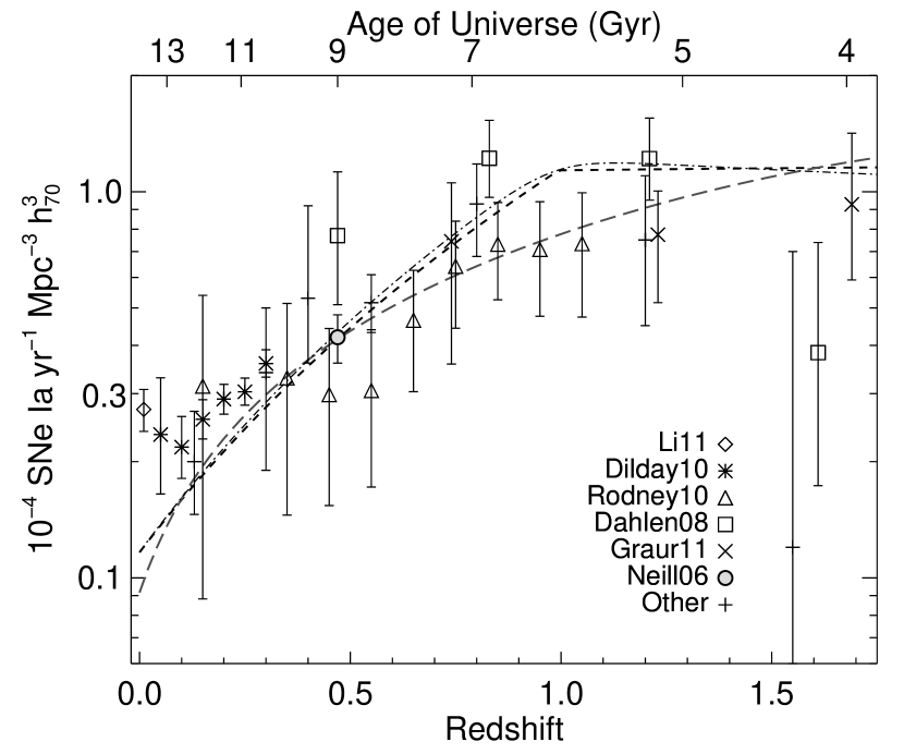
In the past decade, volumetric SN Ia rates have been measured to varying degrees of accuracy out to redshifts of (Fig. 1). Cappellaro et al. (1999) compute the SN Ia rate in the local universe () from a combined visual and photographic sample of galaxies, yet their ability to distinguish core-collapse SNe from Type Ia SNe was severely limited. More recent work by Li et al. (2011b) using SNe Ia from the Lick Observatory Supernova Search (LOSS; Leaman et al., 2011) has made significant improvements in the statistics over previous studies on local SNe Ia. The rates published by Dilday et al. (2010) include data from 516 SNe Ia at redshifts from the SDSS-II Supernova Survey (SDSS-SN), with roughly half of these confirmed through spectroscopy.
At intermediate redshifts, rate measurements are provided by Pain et al. (2002, 38 SNe from the Supernova Cosmology Project in the range ), Tonry et al. (2003, 8 SNe within ), and Rodney & Tonry (2010, SNe from the IfA Deep Survey, 23 of which have spectra). Neill et al. (2006) used a spectroscopic sample of 58 SNe Ia from the first two years of SNLS to measure a cumulative volumetric rate in the redshift range .
SN Ia rates out to are presented by Dahlén et al. (2004) using 25 SNe Ia (19 with spectra) from Hubble Space Telescope (HST) observations of the Great Observatories Origins Deep Survey (GOODS) fields. These data were reanalyzed by Kuznetsova et al. (2008) using a Bayesian identification algorithm, and the HST sample updated by Dahlén et al. (2008) extending the 2004 sample to 56 SNe. Ground-based measurements from the Subaru Deep Field have also been made by Poznanski et al. (2007) using 22 SNe Ia, updated by Graur et al. (2011) with 150 events.
The general trend of Fig. 1 reveals that the rates typically increase from to . There is a wide spread in the existing rate measurements, particularly in the range . At higher redshifts, data from the GOODS collaboration provide some apparent evidence for a turnover in the SN Ia rates. In particular, Dahlén et al. (2004, 2008) report a decline in SN Ia rates beyond . If present, this decline might point to a larger characteristic delay time between star formation and SN explosion (see also Strolger et al., 2004). However, another independent analysis of the HST GOODS data finds rates that are offset, with measurements by Kuznetsova et al. (2008) consistently lower than those of Dahlén et al. (2004, 2008). Kuznetsova et al. (2008) argue that their results do not distinguish between a flat or peaked rate evolution. Ground-based data in this range (Graur et al., 2011), while consistent with the HST-based results, show no obvious evidence for a decline above .
In this paper we use four years of data from the SNLS sample to investigate the evolution of SN Ia rates with redshift out to . The sample presented comprises photometrically identified SNe Ia from SNLS detected with the real-time analysis pipeline (Perrett et al., 2010). One third of these have been typed spectroscopically, and one half of the have a spectroscopic redshift (sometimes from ancillary redshift surveys in the SNLS fields). No other data set currently provides such a well-observed and homogeneous sample over this range in redshift.
Additionally, rigorous computation of the survey detection efficiencies and enhancements in photometric classification techniques are incorporated into the new SNLS rate measurements. Monte Carlo simulations of artificial SNe Ia with a range of intrinsic parameters are performed on all of the detection images used in the SNLS real-time discovery (Perrett et al., 2010); these provide an exhaustive collection of recovery statistics, thereby helping to minimize the effects of systematic errors in the rate measurements.
The SNLS SNe Ia can be used to examine the relationship between the and redshift, given some model of the SN Ia DTD. The size of the SNLS sample also permits a division of the SNe Ia by light-curve width (in particular the “stretch”; see Perlmutter et al., 1997), allowing a search for differences in the volumetric rate evolution expected by any changing demographic in the SN Ia population. Brighter, more slowly-declining (i.e., higher stretch) SNe Ia are more frequently found in star-forming spirals, whereas fainter, faster-declining SNe Ia tend to occur in older stellar populations with little or no star formation (Hamuy et al., 1995; Sullivan et al., 2006b). If the delay time for the formation of the lowest-stretch SNe Ia is sufficiently long (i.e., their progenitors are low-mass stars Gyr old), these SNe Ia will not occur at high redshifts (Howell, 2001). The behavior of the high- rates can reveal the properties of the progenitor systems.
The organization of this paper is as follows: An overview of the rate calculation is provided in §2. The SNLS data set, along with the light-curve fitting and selection cuts used to define the photometric sample, is introduced in §3. SN Ia detection efficiencies and the rate measurements are presented in §4 and §5, respectively. Several models of the SN Ia DTD are then fit to the rate evolution in §6, and the results discussed. Finally, the stretch dependence of the rate evolution is investigated in §7. We adopt a flat cosmology with (,)=(0.27,0.73) and a Hubble constant of .
2 The rate calculation
The volumetric SN Ia rate in a redshift () bin is calculated by summing the inverse of the detection efficiencies, , for each of the SNe Ia in that bin, and dividing by the co-moving volume () appropriate for that bin
| (1) |
The factor corrects for time dilation (i.e., it converts to a rest-frame rate), is the effective search duration in years, and the volume is given by
| (2) |
where is the area of a search field in deg2 and in this equation is the speed of light, and , and are the cosmological parameters, and we assume a flat universe.
is a recovery statistic which describes how each SN Ia event should be weighted relative to the whole population; gives the fraction of similar SNe Ia that exploded during the search interval but that were not detected, for example due to sampling or search inefficiencies. is a function of the SN stretch , a dimensionless number that expands or contracts a template light curve defined as to match a given SN event, the SN color , defined as the rest-frame color at maximum light in the rest-frame -band, and the SN .
The are evaluated separately for each year and field of the survey, and are further multiplied by the sampling time available for finding each object () to convert to a “per year” rate. Typically these are 5 months for the SNLS, though this is dependent on the field and year of the survey. Thus, in practice, eqn. (1) is evaluated for each search field and year that the survey operates.
This “efficiency” method is particularly suited for use with Monte-Carlo simulations of a large, well-controlled survey such as SNLS. Its disadvantage is that it is not straight forward to correct for the likely presence of SNe that are not represented (in parameter space) among the in eqn. (1) (for example, very faint or very red SNe Ia) without resorting to assuming a luminosity function to give the relative fractions of SNe with different properties. In particular, we are not sensitive to, and nor do we correct for, spectroscopically peculiar SNe Ia in the SN2002cx class (e.g., Li et al., 2003), and similar events such as SN2008ha (e.g., Foley et al., 2008), super-Chandrasekhar events (e.g., Howell et al., 2006), and other extremely rare oddballs (e.g., Krisciunas et al., 2011). We also exclude sub-luminous SNe Ia (here defined as , a definition that would include SN1991bg-like events) but note that these are studied in considerable detail for the SNLS sample in our companion paper, González-Gaitán et al. (2011). Thus, we are presenting a measurement of the rates of “normal”, low to moderate extinction SNe Ia (explicitly, ), restricting ourselves to the bulk of the SN Ia population that we can accurately model. We allow for these incompletenesses when comparing to other measurements of the SN Ia rate in §6, which do include some of these classes of SNe Ia.
The photometric sample begins with the set of all possible detections, to which we apply a series of conservative cuts to remove interlopers. The SNLS sample and the culling process are described next in §3. To each resulting SN Ia must then be applied the corresponding ; these are calculated using a detailed set of Monte Carlo simulations on the SNLS images, a procedure described in §4. The rate results and the measurement of their associated errors are presented afterwards in §5.
3 Defining the SNLS sample
In this section, we describe the SNLS search and the SN Ia sample that we will subsequently use for our rate analysis. The SNLS is a rolling SN search that repeatedly targeted four fields (named D1–4) in four filters () using the MegaCam camera (Boulade et al., 2003) on the 3.6 m Canada–France–Hawaii Telescope (CFHT). The SNLS benefited from a multi-year commitment of observing time as part of the CFHT Legacy Survey. Queued-service observations were typically spaced days apart during dark/grey time, yielding epochs on the sky per lunation. Key elements of the SNLS are its consistent and well-defined survey characteristics, and the high-quality follow-up spectroscopy from 8m-class telescopes such as Gemini (Howell et al., 2005; Bronder et al., 2008; Walker et al., 2011), the ESO Very Large Telescope (VLT; Balland et al., 2009), and Keck (Ellis et al., 2008). Due to the finite amount of follow-up observing time available, not all of the SN Ia candidates found by SNLS were allocated for spectroscopic follow-up (for a description of follow-up prioritization, see Sullivan et al., 2006a; Perrett et al., 2010). The availability of well-sampled light curves and color information from the SNLS nonetheless allow us to perform photometric identification and redshift measurements, even in the absence of spectroscopic data.
| Field | RA (J2000) | DEC (J2000) | Area (sq. deg) | Nseasons |
|---|---|---|---|---|
| D1 | 02:26:00.00 | -04:30:00.0 | 0.8822 | 4 |
| D2 | 10:00:28.60 | +02:12:21.0 | 0.9005 | 4 |
| D3 | 14:19:29.01 | +52:40:41.0 | 0.8946 | 4 |
| D4 | 22:15:31.67 | -17:44:05.7 | 0.8802 | 4 |
To identify the photometric SN Ia sample, we begin with all variable object detections in the SNLS real-time pipeline111http://legacy.astro.utoronto.ca (Perrett et al., 2010). Other articles will describe a complementary effort to measure the rates with a re-analysis of all of the SNLS imaging data (e.g., Bazin et al., 2011). We use SNLS data up to and including the fifth year of D3 observing in June, 2007222In June 2007, the filter on MegaCam was damaged during a malfunction of the filter jukebox. Candidates discovered after this period were observed with a new filter, requiring new calibrations for subsequent images, and were thus not included in the present study.. The first (2003) season of D3 is omitted in this analysis; this was a pre-survey phase when the completeness of the SN data differed significantly from the rest of the survey. The remaining detections made during four observing seasons for each of the four deep fields are considered in this analysis. Each period of observation on a given field is called a “field-season”, with 16 field-seasons in total (4 fields observed for 4 seasons). The coordinates of the field centers and other information are provided in Table 1.
We remove all candidates falling within masked regions in the deep stacks. These regions include areas in and around saturated bright stars or galaxies, as well as in the lower signal-to-noise edge regions of the dithered mosaic. The remaining unmasked areas in each field are listed in Table 1, and add up to a total of square degrees. Galaxy catalogs from these image stacks are used to determine the placement of test objects in the simulations described later in §4. This cut therefore ensures that the areas being considered in the rates calculation match those used in the detection efficiency measurements.
We next fit each event with a light curve fitter to determine its redshift (where no spectroscopic redshift is available) and photometric parameters (3.1). We then remove SN Ia candidates with insufficient light curve coverage (§3.2). Finally, we use the light curve fits to identify and remove core-collapse SNe as well as other transients, such as AGN and variable stars (§3.3). Each of the remaining SNe Ia will then correspond to some fraction of the true number of events having similar photometric properties but which were undetected by our survey. This detection efficiency will be determined from the Monte Carlo simulations presented in §4.
3.1 Light-curve fitting
We fit template light curves to the SN Ia candidates to identify those that don’t match typical SNe Ia. Flux measurements are made on all of the final “Elixir-preprocessed” images333CFHT-LS images processed with the Elixir pipeline are available from the Canadian Astronomy Data Centre (CADC): http://www.cadc-ccda.hia-iha.nrc-cnrc.gc.ca/cadc/ (Magnier & Cuillandre, 2004). The Canadian SNLS photometric pipeline (Perrett et al., 2010) was used to measure the SN fluxes, using images processed with the accumulated flat-fields and fringe-maps from each queue run, and aligning photometrically to the tertiary standard stars of Regnault et al. (2009).
Two light-curve fitting tools were used to help identify the SNe Ia: estimate_sn (Sullivan et al., 2006a) for preliminary identification and for measuring SN Ia photometric redshifts, and SiFTO (Conley et al., 2008) for final light-curve fitting to measure the stretch and color of each candidate. The estimate_sn routine is not designed for exact measurement of SN Ia parameters, and SiFTO does not fit for redshift, so we require this two-step process to fully characterize the photometric sample of events.
In estimate_sn, the measured fluxes in are fit using SN Ia spectral templates from Hsiao et al. (2007). The current version of the code includes the addition of priors in stretch, color, and mag. These are determined from the distributions measured for the spectroscopic sample. The photometric redshifts () output from this routine are used for candidates with no available spectroscopic redshifts from either the SN or its host. SiFTO is an empirical light-curve analysis method that works by manipulating a spectral energy distribution (SED) model rather than operating in integrated filter space (Conley et al., 2008). SiFTO does not impose a color model to relate the observed filters during the light-curve fits. The implication of this is that SiFTO cannot easily be modified to fit for redshift, and thus requires a known input . Output SN Ia fits are parameterized by stretch, date of maximum light, and peak flux in each filter.
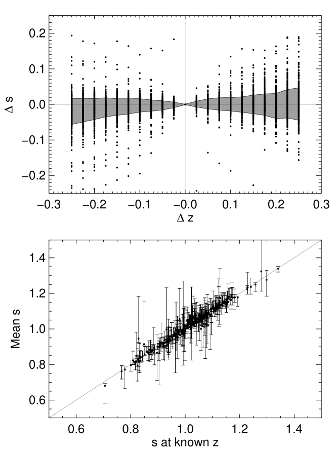
The stretch measurement provided by SiFTO is largely invariant to changes in input redshift, as demonstrated in Fig. 2. Even when the input redshift is off by , the output stretch remains within of its actual value. Opacity effects in the SN ejecta are more pronounced in the bluer bands, causing a more rapid decline (Kasen & Woosley, 2007); light curves measured at shorter wavelengths are therefore intrinsically narrower. As a result, if SiFTO is (for example) given an incorrectly small input redshift, it measures the “wrong” time dilation but simultaneously samples further towards the blue end of the spectrum where the template is intrinsically narrower. The latter effect partially negates the first, resulting in the same stretch measurement regardless of marginal deviations in input redshift. While this is not similarly true of the derived color or measured fit quality, this stretch invariance is extremely useful for establishing an initial constraint in fitting photometric redshifts with estimate_sn.
Spectroscopic redshifts are available for 525 (43%) of the detections remaining after the observational cuts: 420 from SNLS spectroscopy and the rest from host-galaxy measurements (including data from DEEP/DEEP2 (Davis et al., 2003), VVDS (Le Fèvre et al., 2005), zCOSMOS (Lilly et al., 2007), and additional SNLS VLT MOS observations). The external redshifts are assigned based on a simple RA/DEC matching between the SNLS and the redshift catalogues, with a maximum allowed separation of 1.5″. For the SNLS MOS work, the host was identified following the techinques of Sullivan et al. (2006b). The known redshifts are then held fixed in the light-curve fits. We also considered the use of galaxy photometric redshifts for the SNLS fields (e.g. Ilbert et al., 2006). However, though these catalogs have an impressive precision, they tend to be incomplete and untested below a certain galaxy magnitude. SN Ia photometric redshifts do not suffer these problems.
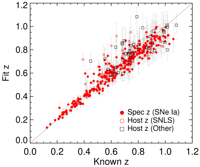
SN photometric redshifts (photo-’s) are calculated for the remaining objects using a multi-step procedure. Preliminary redshift estimates are obtained using a first round of estimate_sn fits without any constraints on the input parameters. The resulting fit redshifts are then used as input to SiFTO to measure the stretch for each object. These stretch values are then fixed in a subsequent round of estimate_sn fits to obtain a more robust measurement of the SN redshift – constraining at least one input parameter to estimate_sn improves the quality of the light-curve fits. Fig. 3 shows that the are in good agreement with the spectroscopic redshifts () out to , with a small systematic offset above that. The median precision in for the confirmed SNe Ia is
with . For comparison, Sullivan et al. (2006a) find with a smaller sample and real-time data (and a previous version of the estimate_sn code). In §5.1, we describe how these errors and the systematic offset are incorporated into the rates analysis.
3.2 Light curve coverage cuts
Each candidate must pass a set of light curve quality checks to be included in the photometric sample of SNe Ia for the rate calculation. Requiring that the SN light curves are well measured ensures that the photometric typing technique is more reliable, and that it is straight forward to correct for the effects of the selection cuts on the rates themselves. Therefore, candidates with insufficient light-curve coverage to measure accurate redshift, stretch, and color values from template fits are removed from the detected sample. We define observational criteria in terms of the phase, , of the SN in effective days (d) relative to maximum light in the rest-frame -band, where
| (3) |
and is the observer-frame phase of the SN. The time of maximum light is determined using the light curve fitter SiFTO (Conley et al., 2008), described in the previous section.
Each object is required to have a minimum of each of the following:
-
•
One observation in each of and between d and d for early light-curve coverage and color information;
-
•
One observation in between d and d for additional color information;
-
•
One observation in each of and between d and d for coverage near peak;
-
•
One observation in either or between d and d to constrain the later stages of the light curve.
These conditions differ slightly from those used by Neill et al. (2006) in their analysis of the first year of SNLS data. Note that no cuts are made on the signal-to-noise (S/N) on a particular epoch; that is, a detection of a candidate on each of the observation epochs is not a requirement. We also neglect the redshift offset seen in Fig. 3 in calculating the above rest-frame epochs. We estimate that this would shift the effective epochs by only one day in the worst case (d; a SN), and in most cases would be far smaller than this.
Table 2 provides the numbers of candidates that survive each of the applied cuts. In total, SNLS detections pass the light curve coverage cuts, of which are spectroscopically confirmed SNe Ia. (For consistency, these same objective requirements are also applied to the artificial SNe Ia used in the Monte Carlo simulations (§4), thereby directly incorporating the effects of this cut into the detection efficiencies.) With these objective criteria satisfied, we can then use light-curve fitting to define a photometric SN Ia sample.
| Cut | All candidates | Confirmed SNe Ia |
|---|---|---|
| Masking cut | 1538 | 325 |
| Observational cuts | 1210 | 305 |
| Fit quality and cuts | 691 | 286 |
3.3 Removing non SNe Ia
A set of goodness-of-fit cuts (here, is the per degree of freedom, ) are applied to all of the SN Ia light-curve fits from estimate_sn to help eliminate non-Ias from the current sample (see also Sullivan et al., 2006a). An overall cut along with individual and filter constraints are applied separately for cases both with and without known redshifts. Light-curve fit quality limits for the sample with known input redshifts are set to , , and (here the is omitted for clarity). Those with fit redshifts are given stricter limits of , , and . The tighter limits for candidates without known redshifts are necessary since core-collapse SNe — specifically SNe Ib/c — can sometimes achieve better fits to SN Ia templates when is permitted to float from the true value. The limits are determined empirically by maximizing the fraction of SNe Ia remaining in the sample, while also maximizing the number of known non-Ias that are removed. Note that estimate_sn, unlike SiFTO, enforces a color relation between the fluxes in different filters, which leads to larger than in SiFTO fits.
In the case of fixed [floating] redshifts input to the fit, [] of spectroscopically identified SNe Ia survive the cuts (we correct for this slight inefficiency when calculating our final rate numbers), while [] of confirmed non-Ias remain in the sample. A final round of SiFTO fits is then performed to determine the output values of stretch and color. The input redshifts to SiFTO are set to wherever no values are available.
One final light-curve fitting cut is then applied on the sample, requiring that the output SiFTO template fits have . This step removes all but one of the remaining confirmed non-Ias444The identification of SNLS-06D4cb is inconclusive, although it has a spectrum that is a poor match to a SN Ia. The SN photometric redshift for this object is but the host has a spectroscopic redshift of . when all redshifts are allowed to float, while at the same time maximizing the number of confirmed SNe Ia passing the cut. No known contaminants remain when all available values are fixed in the fits.
3.4 The photometric SN Ia sample
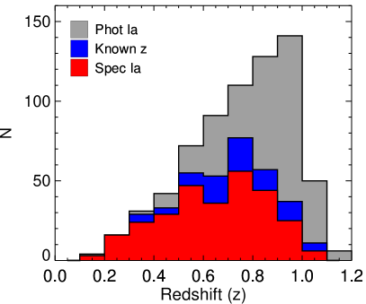
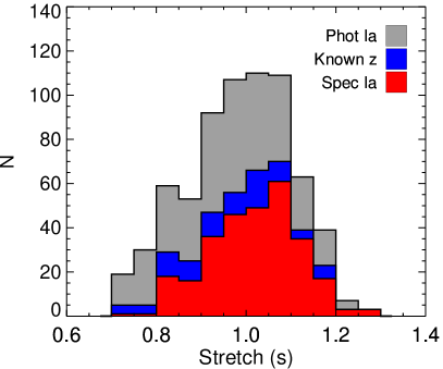
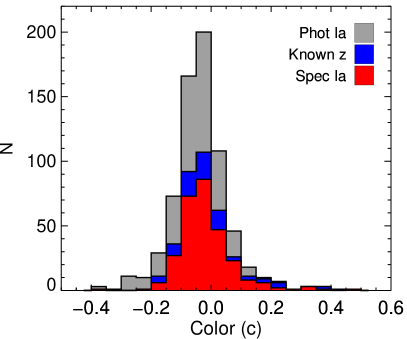
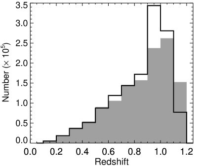
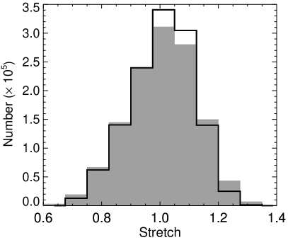
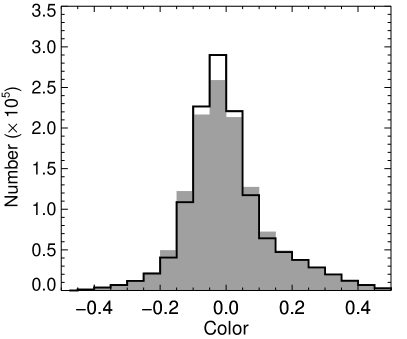
The final photometric SN Ia (phot-Ia) sample is restricted to . Above this redshift, the rates are found to be too uncertain to include in subsequent analyses. This is a result of low S/N, poor detection efficiency, 100% spectroscopic incompleteness, and the potential for increased contamination from non-Ias. Only candidates having stretch values within are considered in the present study. This range is characteristic of the SNLS spectroscopic sample — shown by the red histogram in the central plot of Fig. 4 – but excludes sub-luminous events such as SN1991bg. These sub-luminous, low-stretch SNe Ia in the SNLS sample have been studied in detail by González-Gaitán et al. (2011) – our stretch limit removes 22 such objects from our sample. Extremely red (), and presumably highly extincted, candidates are also removed. This cut eliminates only one event: SNLS-04D2fm, a faint SN of unknown type at .
The final redshift, stretch, and color distributions resulting from the various cuts are shown in Fig. 4. The phot-Ia sample consists of objects, of which have known redshifts. A total of objects in this sample have been spectroscopically confirmed as Type Ia SNe (Table 2). The redshift histogram reveals that the incompleteness of the spectroscopic sample (in red) begins to increase beyond , where the rise in the required exposure time makes taking spectra of every candidate too expensive. The effects of incompleteness in the observed SNLS sample become severe above . The full phot-Ia sample has median stretch and color values of and , respectively. The color distribution peaks at a slightly redder value than the estimated typical color of a SNe Ia of , based on the distribution observed for the spectroscopic SNLS sample.
4 Detection efficiencies
With the final SN Ia sample in hand, we now need to estimate the weight that each of these events contributes in our final rates calculation. These “detection efficiencies” depend on many observational factors and will obviously vary with SN Ia characteristics. For example, at higher-redshift, the higher stretch SNe Ia are more likely to be recovered not only because they are brighter, but also because they spend a longer amount of time near maximum light, and are therefore more likely to pass the culls of 3.2. In a rolling search like SNLS, such effects can be directly accounted for by measuring recovery statistics for a range of simulated input SN Ia properties using the actual images (and their epochs) observed. This is a brute-force approach, but is a practical way to accurately model a survey such as SNLS, helping to control potential systematic errors by avoiding assumptions about image quality limitations and data coverage that may bias the rate calculation. Uncertainties on search time and detection area are avoided since the actual values are well defined.
4.1 Monte Carlo simulations
An exhaustive set of Monte Carlo simulations were performed for each field-season to determine the recovery fraction as a function of redshift, stretch, and color. Full details about these simulations are presented in Perrett et al. (2010).
A total of artificial SNe Ia with a flat redshift distribution were added to galaxies present in the SNLS fields. Each host galaxy was chosen to have a photometric redshift within 0.02 of the artificial SN redshift, with the probability of selecting a particular galaxy weighted by the “A+B” SN rate model with coefficients from Sullivan et al. (2006b, hereafter S06). Within their host galaxies, the artificial SNe were assigned galactocentric positions drawn from the two-dimensional Gaussian distribution about the host centroid returned by SExtractor, i.e., the artificial SNe are placed with a probability that follows the light of the host galaxy.
The simulated objects were assigned random values of stretch from a uniform distribution in the range , with colors calculated from the stretch–color relationships presented in González-Gaitán et al. (2011) (the use of a uniform distribution in stretch ensures that the parameter space of SN Ia events is equally sampled). Peak apparent rest-frame magnitudes () at each selected redshift were calculated for our cosmology and a SN Ia absolute magnitude, and adjusted for the color–luminosity and stretch–luminosity relations. We use an empirical piece-wise stretch-luminosity relationship with different slopes above and below (e.g. Garnavich et al., 2004; González-Gaitán et al., 2011), and SN Ia photometric parameters from the SNLS3 analysis (Conley et al., 2011; Sullivan et al., 2011). These peak apparent magnitudes were then further adjusted by an amount mag according to the observed intrinsic dispersion () in SN Ia magnitudes following and corrections. Here, parameterizes a Gaussian distribution from which a mag can be assigned for each artificial event.
The SN color–luminosity relation includes both effects intrinsic to the SN, and extrinsic effects such as dust. We use coefficients consistent with the SNLS3 analysis, which favor a slope between and of , the value expected based on Milky Way dust. As there is no evidence that this slope evolves with redshift (Conley et al., 2011), we keep it fixed for all the artificial SNe. For the detection efficiency grids, our values range up to 0.6, corresponding to a SN that is mag fainter in -band than a normal SN Ia.
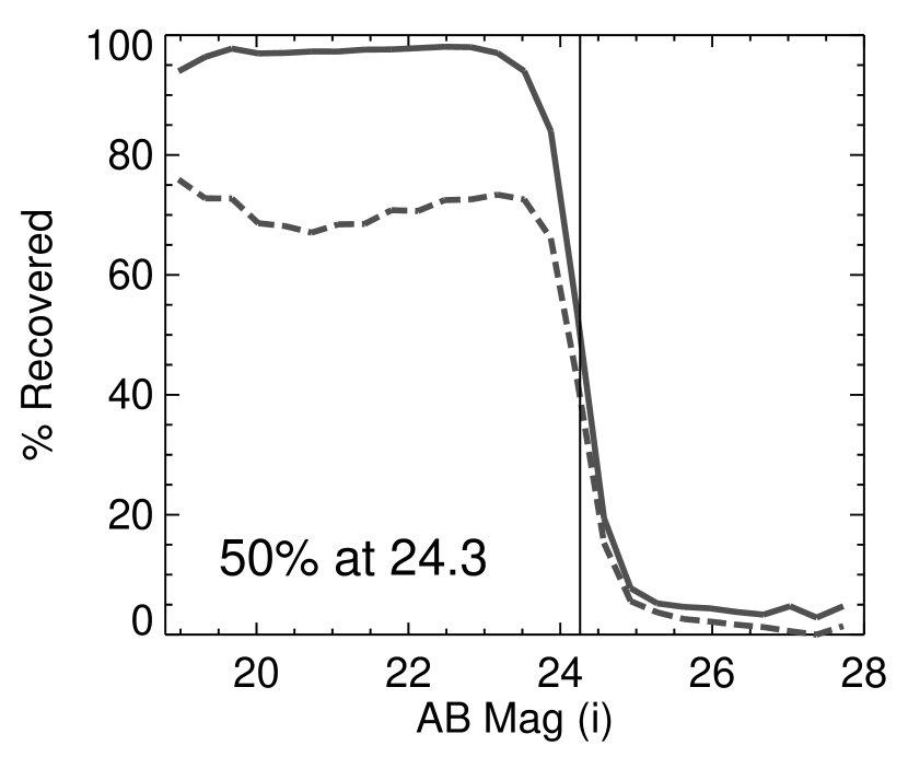
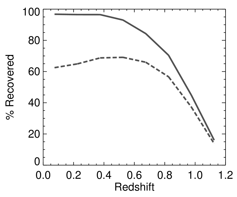
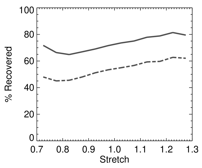
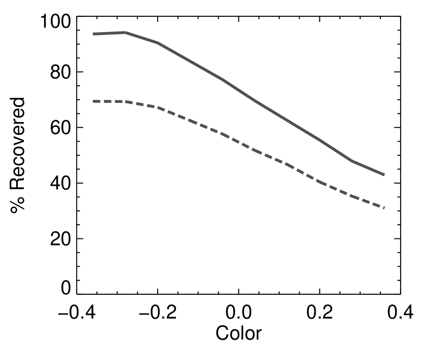
Each artificial SN was assigned a random date of peak magnitude. For the field-season under study, this ranged from 20 observer-frame days before the first observation, to 10 days after the last observation. This ensures that the artificial events sample the entire phase range allowed by the culls in 3.2 at all redshifts. The light curve of each event in was then calculated using the -correction appropriate for each epoch of observation, and each artificial object was added at the appropriate magnitude into every image. The real-time search pipeline (Perrett et al., 2010), the same one that was used to discover the real SNe, was run on each epoch of data to determine the overall recovery fraction as a function of the various SN Ia parameters. The variation in candidate recovery over magnitude, redshift, stretch, and color are shown by the solid lines in Fig. 5. The 50% detection incompleteness limit lies at mag in the AB system.
As expected, SNe Ia that are high stretch, blue, or at lower redshift are all generally easier to recover. Note that at lower redshifts, the faster (less time-dilated) nature of the SN Ia light curves means that the observational criteria of §3.2 are slightly more likely to remove events (as there are fewer opportunities to observe a faster SN), hence the observed decrease in the recovered fraction towards lower-redshifts. That is, a low- SN that peaks during bright time is less likely to be recovered than a higher- SN peaking at the same epoch, even if they had the same observed peak magnitude. This is also partially reflected in the fraction recovered as a function of magnitude, with a curvature in the recovered fraction towards brighter magnitudes. The recovery results are discussed in detail in Perrett et al. (2010).
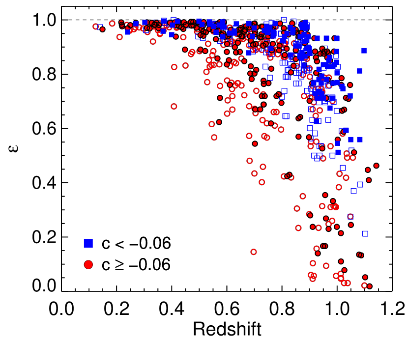
A grid of detection efficiencies was constructed independently for each field-season using the recovery statistics in bins of measured redshift (), stretch (), and color (). These bin sizes were found to provide adequate resolution in each parameter. We investigated the use of a higher resolution in stretch and color, and found no significant on impact our results. Every observed phot-Ia in the SNLS sample is thereby assigned a detection efficiency by linearly interpolating in space that corresponds to the field-season during which it was detected, along with its other measured parameters: . These detection efficiencies are plotted in Fig. 6 prior to any adjustments for sampling time and the availability of observations. Redder, lower-stretch SNe Ia tend to have smaller detection efficiencies, as shown by the open circles in Fig. 6. For clarity, detection efficiency errors are not shown in Fig. 6.
Statistical uncertainties on for well-sampled data are governed by the number of Monte Carlo simulations performed, and are small in comparison to the systematic error resulting from assumptions made about the underlying intrinsic SN Ia magnitude dispersion (the mag distribution, parameterized by ). To estimate these latter errors, the detection efficiencies are recalculated using a range of values from . Bins with will effectively have zero uncertainty, since the likelihood of recovery will not depend on the details of the population distribution; by contrast, “low-efficiency” bins are more seriously affected. These detection efficiency “errors” are included into the overall rate uncertainties in §5.1.
4.2 Sampling time
To remain consistent in the selection criteria used for both the observed SNLS sample and the fake objects, we also apply the same observational cuts described in §3.2 to the artificial SNe Ia. Using the peak date of each simulated light curve, we determine whether the minimum observing requirements are met in each filter by comparing with the SNLS image logs. This directly incorporates the observational cuts into the detection efficiency calculations, while factoring in losses due to adverse weather and the gaps between epochs. The recovery fractions that include these observational requirements are shown by the lower dashed lines in Fig. 5.
Each candidate’s detection efficiency is multiplied by a factor to account for its corresponding sampling time window for detection, yielding a “time corrected” rest-frame efficiency :
| (4) |
The sampling period (in years) for a given field-season is
| (5) |
where MJD is the modified Julian date of the available detection images. The extra 30 days account for the range in peak dates allowed for the artificial SN Ia light curves, from 20 days prior to the first observation in a given field-season to 10 days past the final epoch.
The resulting time-corrected rest-frame detection efficiencies for the phot-Ia sample are plotted as a function of redshift in Fig. 7. Since each field is observable for at most months of the year, peaks at even for bright, nearby objects.
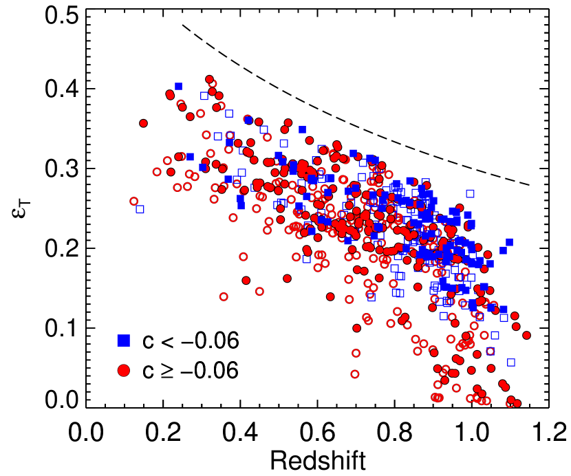
Figs. 6 and 7 show that there is a drop-off in the efficiencies above , in particular for the redder bins, making it more difficult to calculate accurate rates at these redshifts due to color–stretch bins which are not sampled. At , it is not possible to measure SN Ia rates using this method due to poor survey sensitivity and inadequate statistical sampling of spectral templates. Therefore, we restrict our volumetric rate calculations to the range .
5 SN Ia rates
Volumetric SN Ia rates are calculated from eqn. 1 by summing the observed SNe Ia weighted by the inverse of their time-corrected rest-frame efficiencies. The total sampling volumes for the deep fields in redshift bins of (eqn. 2) are provided in Column 2 of Table 3. Columns 3 and 4 show the numbers of observed candidates in each bin for the entire sample () and for the spectroscopically confirmed SNe Ia () in each redshift bin. The “raw” measured rates () with their weighted statistical errors are given in Column 5, in units of ; see later sections for the meaning of the remaining columns.
| bin | Survey Volume | aaThe first error listed is statistical, and the second systematic. | |||||
|---|---|---|---|---|---|---|---|
| ( Mpc3) | () | () | |||||
| 17.3 | 4 | 3 | 0.16 | ||||
| 42.8 | 16 | 16 | 0.26 | ||||
| 75.7 | 31 | 24 | 0.35 | ||||
| 112.7 | 42 | 29 | 0.45 | ||||
| 151.5 | 72 | 47 | 0.55 | ||||
| 190.1 | 91 | 36 | 0.65 | ||||
| 227.2 | 110 | 56 | 0.75 | ||||
| 262.1 | 128 | 44 | 0.85 | ||||
| 294.1 | 141 | 25 | 0.95 | ||||
| bbBins at are not included in the rates analysis; see Section 5.2 | 323.0 | 50 | 6 | 1.05 | |||
Contamination by non-Ias that survive the culling criteria is estimated to contribute under to the total measured rates to . The contribution is found to be negligible up to , at which point it increases to around at . This is determined by summing for the known non-Ias, and dividing by the corresponding value for objects in each redshift bin with available spectroscopy. The values used here are based on the results obtained when allowing redshift to vary in the fits, not when holding fixed at the spectroscopic redshifts.
We now correct the raw measured rates for potential systematic offsets in the photometric redshifts and other parameters. This is done using the technique described next in §5.1, which also computes a combined statistical and systematic uncertainty on the final rates. The SN Ia rates are potentially also sensitive to the inclusion of very low detection efficiency candidates at , and we must consider the effects of undetected SNe Ia in bins with very poor detection recovery rates. These low-efficiency issues are discussed later in §5.2.
5.1 Error analysis
In addition to the simple “root-” statistical errors, a number of additional uncertainties also affect our measured rates. These can include errors in the measured SN (photometric) redshift, stretch, and color, which together determine the detection efficiency (and hence weight) assigned to each event.
As shown in Fig. 3, there is a redshift uncertainty in each measure of . The discrepancy between and for the confirmed SN Ia sample is presented in Fig. 8 for two bins in stretch. There is a small offset above , increasing to () at in the sample, and () in the sample. On average, the measurements are underestimated, with an increasing offset to higher redshift.
An offset is expected based on a Malmquist bias, such that brighter objects are more likely to have a spectroscopic type at a fixed redshift (Perrett et al., 2010). However, we estimate this effect to be smaller: the solid lines in Fig. 8 show this predicted offset as a function of redshift. This is calculated by estimating the rest-frame -band apparent magnitude with for the adopted cosmology, and applying the mag offsets contributed by spectroscopic selection as measured in Perrett et al. (2010).


To study these various uncertainties, and to handle this redshift migration effectively, we perform a set of Monte Carlo simulations on the measured rates. We begin with the basic rate measurements, , from Table 3, and calculate how many measured SNe Ia that rate represents in each redshift bin by multiplying by the volume in that bin: . Many realizations (5000) are performed by drawing objects from typical SNLS-like distributions of artificial SNe Ia. These are the same artificial objects as used in the detection efficiency calculations (§4), although the stretch, color, and mag distributions are matched to those of the spectroscopically confirmed SN Ia sample (see Perrett et al., 2010). The distributions for input to the error calculations are shown in Fig. 9. Only a fraction of the objects in each redshift bin have a spectroscopic redshift, with the remainder having a SN Ia photometric redshift and accompanying uncertainty (Fig. 8). This “spectroscopic fraction”, is calculated in each redshift bin from Fig. 4.

The procedure for each realization is then as follows:
-
1.
is randomized according to the Poisson distribution, using the Poisson error based on but scaled to , to give simulated objects.
-
2.
Each simulated object in each redshift bin is assigned a random redshift appropriate for that bin (). Within each bin, the probability follows a scaled number-density profile according to the expected increase in volume with redshift.
-
3.
The are then randomly matched to a SN Ia from the artificial distribution with the same redshift (Fig. 9), and that event’s stretch () and color () assigned to the simulated event.
-
4.
Using the fraction of spectroscopic redshifts in each bin (Fig. 4), we assign this fraction of the objects to correspond to a spectroscopic redshift measurement. The remaining redshifts are assumed to come from a photometric fit, and are shifted and randomized using the median offsets and standard deviations shown in Fig. 8 to give . Any event with a is not adjusted.
-
5.
Correlated stretch and color errors are then incorporated for all objects, using typical covariances produced by SiFTO for the SNLS sample, and the and randomized to and .
-
6.
, , and are used to match each simulated object to a detection efficiency. Efficiency errors are included by applying a random shift drawn from an two-sided Gaussian representing the asymmetric uncertainties on each value (§4.1).
-
7.
Random numbers between zero and one are generated to evaluate whether each simulated object gets “found”: if the selected number is lower than the detection efficiency associated with the simulated object, that event is added to the rate calculated for that iteration.
-
8.
The rate for that iteration is then calculated using the appropriate detection efficiencies from step 6.
The final volumetric rates are presented in Columns 7 of Table 3. These are calculated as the mean of the 5000 simulated rates in each redshift bin. We also calculate the standard deviation in each bin, subtract from this in quadrature the statistical Poisson uncertainty based on , with the remainder our estimate of the systematic uncertainty in each redshift bin.
The effects of the simulations described above on the input redshift, stretch, and color distributions are shown in Fig. 10. The redshift histogram shows that the offsets applied in step 4 of the simulations produce a net increase in redshift to compensate for the small bias in the photometric fitting, with the effect increasing towards higher . This causes a flattening of the output rates calculated by the simulations as compared with the measured (and uncorrected) rates (Table 3). In addition to the offset towards higher redshifts at , there is also a very small spread in the stretch and color distributions (Fig. 10).
5.2 Low-efficiency candidates
The detection efficiencies in some of the reddest bins begin to rapidly decrease at (Fig. 7). As the contribution to the rate from each observed SN Ia goes as , the measured volumetric rates are particularly sensitive to any objects with very low detection efficiencies (). There is also the potential for a complete omission of SNe Ia in some bins. For example, in bins with less than detection efficiency, on average at least 10 SNe Ia must be observable in a given field-season for just one to be detected. If that one SN is not detected by the real-time pipeline, the 10 SNe Ia that it truly represents in that bin will never be counted in the final rates tally (and the rate measurement will be biased).
To examine the sensitivity of our rates on the “low- regions” of parameter space, we use the detection-efficiency-corrected SNLS sample as a model for the true (, ) SN Ia distribution at . This population is assumed observationally complete (Fig. 5) and is taken to be representative of the underlying sample of SNe Ia in the universe555Of course, this relies on the (possibly incorrect) assumption of no evolution in intrinsic stretch or color as a function of redshift (e.g., Howell et al., 2007).. The two-dimensional (, ) distribution at is fit to the five bins, and the best-fit scaling determined. The total rates are then calculated from those scaled numbers (tabulated in Table 3)
These tests indicate that, while the results remain consistent within their errors up to ( compared with ), there is a significant amount of uncertainty in the SNLS rates at higher redshifts due to sample incompleteness. At , the scaled rate is , whereas our the calculated value is . This finding is consistent with the results shown in Figs. 4 and 6: the phot-Ia sample numbers drop significantly at , and those that are found in the sample can have very low . For these reasons, we limit the formal analysis of the SNLS rates to .
6 Delay-time distributions
Having measured volumetric SN Ia rates and associated errors, we now compare our measurements with those of other studies. We also examine the SN Ia rate evolution as a function of redshift, and compare with predictions based on various simple delay-time distribution models from the literature.
For comparison of the SNLS rate measurements to various SN Ia models, additional data in redshift ranges not sampled by SNLS is required. In the rest of this section, we will make use of an extended SN Ia rate sample comprising the Li et al. (2011b) LOSS measurement at , the Dilday et al. (2010) sample from SDSS-SN at , and the recent Graur et al. (2011) Subaru Deep Field (SDF) sample at higher redshifts, together with our SNLS results. Clearly other samples could have been chosen – however, these three are the largest SN Ia samples in their respective redshift ranges, and have the greatest statistical power. In the case of the SDSS and SDF samples, they are also built on rolling SN searches similar to SNLS.
We make some small corrections to these published rates in order to ensure a fair comparison across samples. The Li et al. (2011b) sample includes all sub-classes of SNe Ia, including the peculiar events in the SN2002cx-like class and sub-luminous events in the SN1991bg-like class. SN2002cx-like events make up 5% of the LOSS volume-limited SN Ia sample (Li et al., 2011a). These are not present (or accounted for) in the SNLS sample, and are excluded from the SDSS analysis (Dilday et al., 2008), so we therefore exclude these from the Li et al. (2011b) sample, reducing their published rate value by 5%.
Both the Li et al. (2011b) and Dilday et al. (2010) samples include SNe Ia in the sub-luminous SN1991bg category (see also Dilday et al., 2008), which we exclude here in the SNLS analysis (these are studied in González-Gaitán et al., 2011). While we could correct our own rates for this population using the González-Gaitán et al. (2011) results, it is unclear how to treat the SDF sample in the same way (do SN1991bg-like events even occur at ?) and the SNLS sub-luminous measurement is quite noisy. Instead we use the very well-measured fraction of SN1991bg-like SNe in the volume-limited LOSS sample (15%), and reduce both the LOSS and SDSS published rates by this amount. This 15% is based on the classifications given in Li et al. (2011b). We confirm that this is appropriate for our stretch selection (i.e., we require ) by fitting the available Li et al. (2011b) light curves with SiFTO. 16% of the available Li et al. (2011b) sample has a fitted stretch , consistent with the 15% reported as 91bg-like by Li et al. (2011b).
6.1 Comparison with published rates
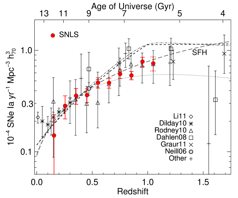
Fig. 11 shows the SNLS volumetric SN Ia rates for comparison with recent published results. The SNLS volumetric rate at published by Neill et al. (2006) is , consistent with our binned rates in the same redshift range. Note that the effects of non-Ia contamination (§5) have not been incorporated into the SNLS errors shown in Fig. 11. Our results are also consistent with Dilday et al. (2010) at , and with Rodney & Tonry (2010) at higher redshifts, although those latter measurements have significantly greater uncertainties.

The SNLS rates show a rise out to , with no evidence of a rollover at . We can parameterize the SNLS rate evolution as a simple power-law:
| (6) |
with the best-fit shown as the solid line in Fig. 12. We find and (all errors in this section are statistical only). This evolution is shallower than a typical fit to the cosmic star-formation history, with (e.g. Li, 2008), though the constraining power of the SNLS data alone at is not great. By comparison, Dilday et al. (2010) find and using the lower-redshift SDSS-SN data, completely consistent with our results. Including all the external data gives and .
6.2 Comparison with delay-time distribution models
| Li (2008) piece-wise SFH | Li (2008) “Cole et al.” SFH | Yüksel et al. (2008) SFH | |||||||||
|---|---|---|---|---|---|---|---|---|---|---|---|
| Data | Model | Fit parameters | Fit parameters | Fit parameters | |||||||
| (Gyr) | (Gyr) | (Gyr) | |||||||||
| ExtendedaaThe extended sample refers to the SNLS sample plus the external data described in 6. | Gaussian | 18 | 3.4 | 2.62 | 3.4 | 1.60 | 3.4 | 3.29 | |||
| Extended | Gaussian | 17 | 2.64 | 1.60 | 3.00 | ||||||
| Ext.+D08 | Gaussian | 19 | 3.4 | 2.72 | 3.4 | 1.68 | 3.4 | 3.43 | |||
| SNLS | Power law | 8 | 1 | 0.76 | 1 | 1.36 | 1 | 0.81 | |||
| Extended | Power law | 18 | 1 | 0.72 | 1 | 1.06 | 1 | 0.78 | |||
| Extended | Power law | 17 | 0.76 | 0.92 | 0.81 | ||||||
| (Gyr) | (Gyr) | (Gyr) | |||||||||
| SNLS | Exponential | 7 | 0.85 | 0.58 | 0.91 | ||||||
| Extended | Exponential | 17 | 1.33 | 1.15 | 1.44 | ||||||
| SNLS | PHS | 8 | 0.5 | 4.14 | 0.5 | 4.81 | 0.5 | 4.31 | |||
| Extended | PHS | 18 | 0.5 | 4.08 | 0.5 | 4.77 | 0.5 | 4.19 | |||
| aaThe extended sample refers to the SNLS sample plus the external data described in 6. | bbUnits of , where refers to the current stellar mass, . | ||||||||||
| SNLS | 7 | 0.74 | 0.59 | 0.78 | |||||||
| Extended | 17 | 0.60 | 0.77 | 0.63 | |||||||
| SNLS | 8 | 0 | 1.81 | 0 | 0.54 | 0 | 1.92 | ||||
| Extended | 18 | 0 | 6.22 | 0 | 2.95 | 0 | 6.70 | ||||
| SNLS | 8 | 0 | 9.72 | 0 | 9.74 | 0 | 10.09 | ||||
| Extended | 18 | 0 | 9.42 | 0 | 9.56 | 0 | 9.66 | ||||
| ccUnits of . | |||||||||||
| Extended | 2-binddUnits of , where refers to the total formed stellar mass, . | 17 | 0.64 | 0.79 | 0.67 | ||||||
We now compare our rate evolution with simple parameterizations of the delay-time distribution (DTD) from the literature relating the cosmic star-formation history (SFH) to SN Ia rates. The DTD, , gives the SN Ia rate as a function of time for a simple stellar population (SSP), i.e., following a -function burst of star formation. The SN Ia rate () at time is then
| (7) |
where SFR() is the star-formation rate as a function of time. Thus, different functional forms of the DTD can be tested against observations of volumetric rates if the SFR(), or the cosmic SFH, is known (e.g., Madau et al., 1998; Strolger et al., 2004; Oda et al., 2008; Horiuchi & Beacom, 2010; Graur et al., 2011). An implicit assumption in this test is that the DTD is invariant with redshift and environment.
As our default SFH model, we choose the Li (2008) update to the Hopkins & Beacom (2006) fit to a compilation of recent star-formation density measures. For simplicity we use a Salpeter (1955) initial mass function (IMF) with mass cut-offs at 0.1 and 100, and assume that stars began to form at . The default SFH is parameterized in a piece-wise fashion, and is over-plotted on the data in Fig. 11. As shown by Förster et al. (2006) and Graur et al. (2011), the choice of SFH can add an additional significant systematic uncertainty in any comparisons of DTDs to SN Ia volumetric data. We therefore compare with results obtained using an alternative parameterization of the SFH by Li (2008) following Cole et al. (2001), as well as a SFH fit to slightly different data by Yüksel et al. (2008) (see also Horiuchi & Beacom, 2010). In 6.3, we also investigate a SFH derived in a very different manner (Wilkins et al., 2008).
The integral of the DTD gives the total number of SNe Ia per formed stellar mass, . This can be converted into the fraction of intermediate-mass stars that explode as SNe Ia, , by multiplying by a factor of 47.2 (for the Salpeter IMF). This assumes that the progenitor mass range for a SN Ia is 3–8 (see Maoz, 2008, for a discussion). For all our model DTDs, we set the DTD to zero at epochs earlier than 40Myr, the approximate lifetime of an star.
6.2.1 Gaussian DTDs
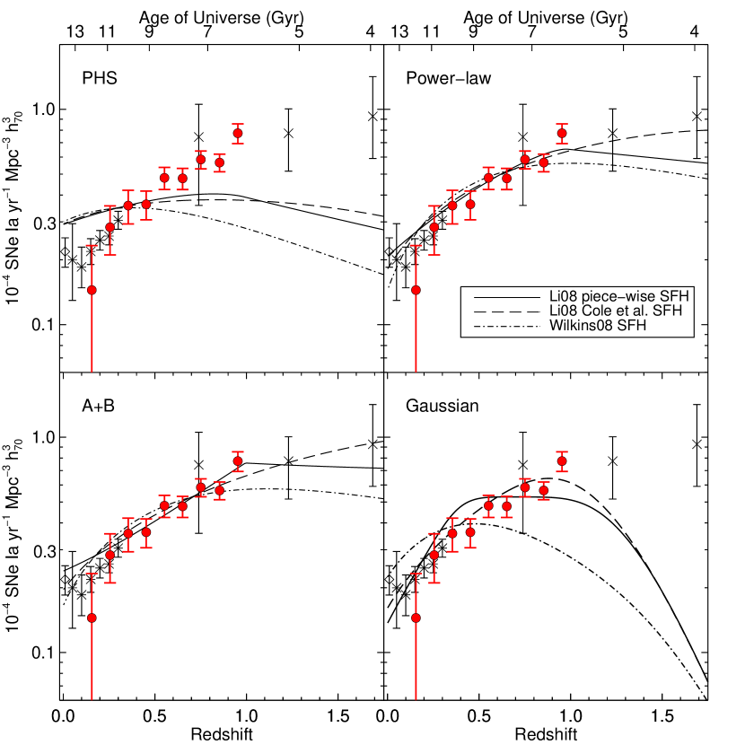
We begin by fitting a Gaussian DTD, with , to the volumetric data, following Strolger et al. (2004) (see also Strolger et al., 2010). We fit a DTD with parameters fixed at Gyr and (i.e., just adjusting the normalization in the fits), as well as a DTD fit with allowed to vary. The results are listed in Table 4 and compared to other DTD fits in Fig. 13.
This model has ( is the reduced , the per degree of freedom, ). Allowing as a free parameter in the fits gives Gyr with a similar – the fit quality is slightly better when using Cole et al. form of the SFH ().
The Gaussian DTDs therefore provide poor fits to the data, and are not capable of matching the SNLS, SDF and SDSS/LOSS data simultaneously. In particular, these Gaussian DTDs predict a decrease in the number of SNe at not seen in the combined data set. However, they were originally favored following fits to data including points from HST searches (Dahlén et al., 2004, 2008) which are not included in our analysis due to their lower statistical precision compared to the SDF study. As a consistency check we also replace the SDF data with the Dahlén et al. (2008) data (adjusted downwards by 15% to account for 19bg-lie events) in our fits – we find that the does not improve (Table 4).
6.2.2 Power law and exponential DTDs
Theoretically, if SNe Ia are dominated by a single channel, the DTD will likely decline with age. In the single degenerate channel, SNe Ia at 10 Gyr should be rare, since 1 secondaries have small envelopes to donate and must rely on only the most massive primaries (Greggio, 2005). A power law DTD (i.e., with ) with a low time-delay cut-off is expected in the double degenerate scenario (e.g. Greggio, 2005; Förster et al., 2006; Maoz et al., 2010), and has been explained post-hoc in the single degenerate channel using a mixture of contributions (Hachisu et al., 2008). Furthermore, models with seem to provide a good match to a variety of recent observational data (Totani et al., 2008; Maoz et al., 2010; Graur et al., 2011).
We fit both and free DTDs to the SNLS+external data. The results can be found in Table 4 and Fig. 13. Our best-fit value is (), consistent with . This broad agreement with holds when considering the other SFH paramterizations ( for the Cole et al. form).
Pritchet et al. (2008, hereafter PHS) present a simple model relating white dwarf formation rate, which decreases with time following an instantaneous burst of star formation as , resulting in a DTD with . By fitting the SN Ia host galaxy data of S06, PHS demonstrate that , irrespective of the assumed SFH or the detailed mixture of stellar populations. PHS argue that the single-degenerate formation scenario alone is not sufficient to account for all of the observed SNe Ia (see also Greggio, 2005). The PHS model makes an explicit prediction for the evolution of the SN Ia rate with redshift, given an input SFH. We fit the PHS model – essentially – to the data and show the resultant fit in Fig. 13 (also Table 3). We find a , obviously a substantially poorer fit than the generic power-law fit, or power-law DTDs with .
For completeness we also also test an exponential DTD, i.e., . When is small, this approximates a simple star-formation dependence, and when large, it approximates a constant DTD. The results are in Table 4; generally, single exponential DTDs provide poor fits to the data, but do still have acceptable .
6.2.3 “Two-component” models
Finally, we examine various two-component DTD models. The first is the popular “” model, a simple, two-component model of SN Ia production that is comprised of a “prompt” component that tracks the instantaneous SFR, and a “delayed” (or “tardy”) component that is proportional to (Mannucci et al., 2005; Scannapieco & Bildsten, 2005):
| (8) |
Here, the and coefficients scale the and SFR components, respectively. The prompt component consists of very young SNe Ia that explode relatively soon (in the model, immediately) after the formation of their progenitors, whereas the delayed component (scaled by ) corresponds to longer delay times and an underlying old stellar population. This model is empirically attractive due to the ease of comparison with readily observable galaxy quantities, such as and SFR. Note that this A+B model does not exactly correspond to a DTD – however, it can be easily converted to a DTD by using the variation of with time in a SSP. This leads to a DTD with some fraction of SNe Ia formed immediately (the component), followed by a slightly decreasing fraction to large times (the component). This decrease is % from 0.1 to 5 Gyr, and % from 1 Gyr to 10 Gyr – clearly significantly shallower than a power law.
Some confusion exists over the exact definition of in eqn. (8), and hence the definition of . Some authors (e.g. Neill et al., 2006) simply treat as the integral of the SFH, equating it to the total formed mass, . Others make corrections for stars that have died, particularly in studies which perform analyses on a galaxy-by-galaxy basis as this quantity is more straight forward to link to observational data (e.g., Sullivan et al., 2006b). This latter definition leads to larger values, as will be less than (see Fig. 7 of S06, for the size of this difference). Here, our values refer to , and we pass the cosmic SFH through the PÉGASE.2 routine (Le Borgne et al., 2004), convolving the chosen SFH with a single stellar population, and generating a galaxy SED from which mass can be estimated. The evolving and SFR are used to perform a fit of equation 8 to the volumetric rate evolution, with results listed in Table 4.
Fitting the SNLS rates alone gives coefficients of and for the Li (2008) piece-wise SFH, with for . Incorporating the external SN Ia rate from LOSS, SDSS and SDF yields values of and , with . This fit is compared to other DTDs in Fig. 13.
Next, we set to investigate the possibility of a pure star-formation dependence, fitting only the prompt () component to the SNLS data. This results in an upper limit of (), equivalent to the normalized SFH curve plotted in Fig. 11. Adding the external data rates to the SNLS values gives an upper limit of , but again with a very poor fit quality (). While the SNLS results themselves are marginally consistent with a pure prompt component (Table 4), adding the additional constraints supplied by the low- data yield a very poor fit. The related test of setting and testing for only the delayed component similarly gives very poor fit results (Table 4).
As discussed above, these and values depend on the adopted SFH. Even ignoring the systematics in the individual SFR measurements to which the SFH model is fit, the type of fit used also introduces considerable uncertainty. Using the Cole et al. form of the SFH, for example, changes the best-fit values to and , a significant variation with similar quality fit than for the piece-wise form. Thus care must be taking in comparing any particular values, or any particular prediction of SN Ia rate evolution, without ensuring the consistent use of a SFH and derivation of .
Clearly, and as well documented in the literature, the model must be a significant approximation to the physical reality in SN Ia progenitor systems. In particular, there must be some delay time for the prompt component, and it is unlikely to act as a delta function in the DTD. We test this by approximating as two discrete bins in time, i.e., a step function with a value at times , and at . We choose Myr (following, e.g., Brandt et al. 2010), and used a sigmoid function to ensure the DTD was continuous when crossing . This DTD also provides a good fit to the data (Table 4), with a significant detection of the two components – and are at 5 in all three SFHs considered (and typically ). We experimented with making this function more general, by allowing to vary. However, these fits were not constraining, although they prefer Gyr, and the fit parameters are highly correlated (i.e., as decreases, increases to ensure a similar fraction of SNe Ia are generated from the “prompt” component).
One direct outcome of this simple two-bin DTD model is that, for our default cosmic SFH, while % of SNe Ia originate from the prompt component integrated over cosmic time, at the prompt component accounts for only % of SNe Ia. These fractions remain fairly constant out to Gyr.
6.3 Discussion
We now compare our DTDs inferred from the volumetric data with other independent estimates from the literature, comparing both the parametric form of our best-fit DTDs, as well as the normalization. In Fig. 14, we plot our inferred DTDs, with normalizations from the best-fits to the volumetric SN Ia rates, and compare to other empirical determinations of the DTD from the literature from a variety of methods (Brandt et al., 2010; Maoz et al., 2010, 2011). The data points come from the analysis of SN Ia rates in galaxy clusters (Maoz et al., 2010), the reconstruction of the DTD from an analysis of the LOSS SN Ia host galaxy spectra (Maoz et al., 2011), and a similar analysis of the host galaxies of SDSS SNe Ia (Brandt et al., 2010).
Where necessary we convert these external measurements to a Salpeter IMF – from a diet-Salpeter IMF (Bell et al., 2003) for Maoz et al. (2010, 2011) and a Kroupa (2007) IMF for Brandt et al. (2010). We also adjust the Maoz et al. (2010) and Maoz et al. (2011) results downwards as their measurements presumably include SN1991bg-like events which are not included in our SNLS analysis (the Brandt et al. analysis does not include these SNe, and their stretch range is well matched to our analysis – see their figure 2). Furthermore, we correct the Brandt et al. (2010) DTD points upwards by 0.26 dex to account for stellar masses in Brandt et al. that are 0.26 dex too high due to a normalization issue in the VESPA code used to derive them (D. Maoz, private communication; R. Tojeiro, private communication).
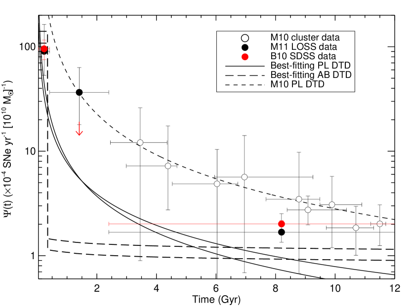
Although the generic shape of the power-law DTD inferred from the volumetric rate data matches the external DTD data well (Fig. 14), it is clear that the best-fit normalization required to reproduce the volumetric rate data differs to that required to fit some of the external samples. The DTDs inferred from volumetric rate data are generally consistent with the Brandt et al. (2010) analysis, and the first and third bins of the Maoz et al. (2011) data.
However, the normalization of the best-fit DTD to the Maoz et al. (2010) cluster data lies significantly above our best-fit DTD. Integrating our best-fit power-law DTDs gives (%) depending on the SFH, in good agreement with similar analyses (Horiuchi & Beacom, 2010). However, this is significantly below the value of obtained by integrating the Maoz et al. (2010) “optimal iron-constraint” power-law DTD (for our IMF), or from the “minimal iron constraint” DTD. We can sanity check our normalizations by predicting the SN Ia rate in the Milky Way, given our DTD values. Assuming a Milky Way stellar mass of and a SFR of , our DTDs give a predicted Milky Way normal SN Ia rate of 0.22-0.25 events per century. This is in good agreement with independent estimates of the actual rate ( to events per century; e.g., Tammann, 1994; Roland et al., 2006; Li et al., 2011a) given the uncertainties involved.
So why is the normalization in the Maoz et al. (2010) cluster SN Ia DTD (which is not arbitrary) different to those derived from volumetric rate data by such a large factor? Several possibilities exist that may explain the discrepancy. The first is that the SNLS, and by extension all other studies, are missing a significant number of SNe Ia, a factor of at least four. However, it is difficult to understand how this might occur, given some of the cluster rates used in Maoz et al. (2010) are drawn from very similar surveys (including SNLS and SDSS-SN).
A second possibility is that the cosmic SFH models used in our analysis over-predict the actual SFR – a lower SFH normalization would require a higher DTD normalization to match the volumetric rate data. To test this possibility, we repeat our rates fitting analysis using the SFH of Wilkins et al. (2008), a SFH derived from a requirement to match the redshift evolution of . Although this agrees with other SFH estimates at , it suggests that high-redshift SFRs could be dex lower compared to the models used in this paper. However, even using this SFH, the integrated power-law DTD only gives (%), still some distance short of that apparently required by the clusters analysis.
Other options to adjust the SFH normalization downward, such as reducing the dust extinction corrections applied to the various star-formation indicators which make up the SFH compilations, are probably not viable given the long-established and significant evidence for obscuration in star-forming galaxies, and the agreement between the different diagnostics (see discussion in Hopkins & Beacom, 2006; Li, 2008).
A third possibility is that the cluster rates used to derive the DTD of Maoz et al. (2010) have some contamination from “younger” SNe Ia, thus increasing their rates above that appropriate for their age, assuming a redshift of formation of 3. This, and other similar potential systematics from the clusters analysis, are discussed in detail in Maoz et al. (2010).
Finally, it may well be the case that the assumption of a single DTD is not adequate, given the various indications that there may be more than one progenitor channel. This would suggest that there is not one universal DTD that is independent of redshift, or other variables, such as metallicity.
7 Stretch dependence
There is an observed correlation between the photometric properties of SNe Ia and their host environments (Hamuy et al., 1995, 2000; Sullivan et al., 2006b). Brighter SNe Ia with slower light-curves tend to originate in late-type spiral galaxies, such that the rates of higher-stretch objects are proportional to star-formation on short ( Gyr) timescales (S06). Meanwhile, fainter, faster-declining SNe Ia are more likely to be associated with older stellar populations. This split seems to extend to the recovered DTDs – Brandt et al. (2010) show that the recovered DTD for low and high stretch SNe Ia are very different, consistent with the above picture of young SNe Ia being high stretch and old SNe Ia low stretch. A larger fraction of high-stretch SNe Ia might therefore be expected at high redshift tracking the increase in the cosmic SFH and hence preponderance of younger stars. Indeed, Howell et al. (2007) find a modest increase in the average light-curve width out to redshifts of . The rate evolution for low-stretch SNe Ia should therefore demonstrate a correspondingly shallower increase with redshift than that of higher-stretch objects.
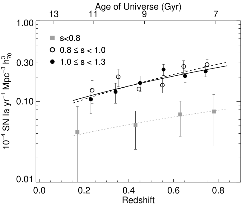
We investigate this trend in Fig. 15, splitting the SNLS sample at the median stretch value of . The measured rates with simple weighted errors are plotted separately for objects with (open circles) and those with (filled circles). We also show the rate measurement from González-Gaitán et al. (2011). The samples from the analysis in this paper exhibit a comparable rise in their rates with redshift, with power-law slopes of and . Extrapolating the fits to each of the samples back to gives the following fractions of SNe Ia at in each group: 17% (), 39% (), and 44% (). The fraction is consistent with the LOSS SN1991bg-like fraction of 15% (Li et al., 2011a), given that true 1991bg-like events have fitted stretches (González-Gaitán et al., 2011). The fraction of very low stretch events with SNe Ia shows only a small increase with increasing redshift (see also González-Gaitán et al., 2011), although the uncertainties are very large.
The stretch-split rates are only considered out to , beyond which redshift the stretch errors become large (), and the lower efficiencies of the redder, lower-stretch SNe Ia can bias the observed stretch evolution by driving up the rates (Fig. 7).
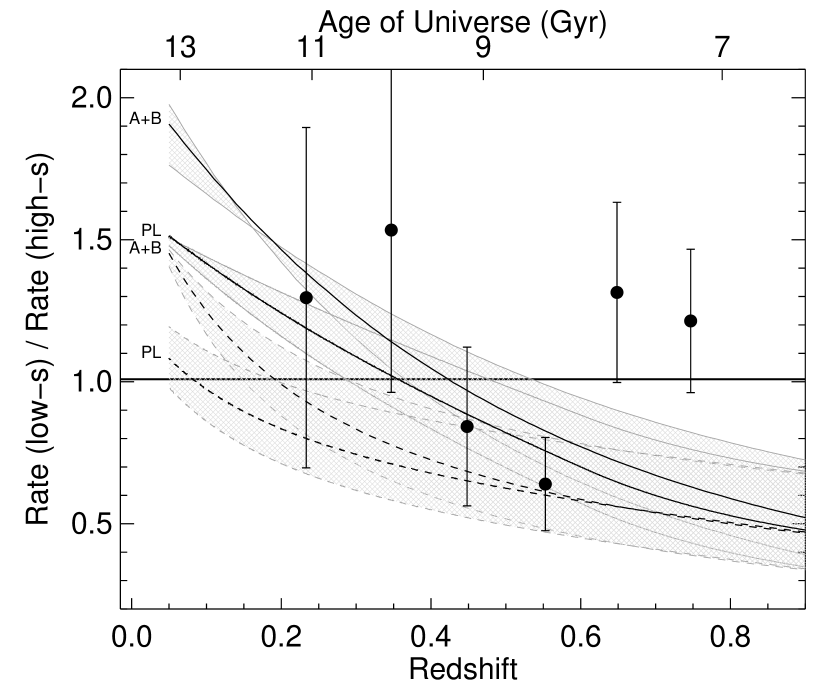
Fig. 16 shows the ratio of the rates split by stretch for . To compare this observed data with any expected evolution, we need model stretch distributions for “old” and “young” SNe, together with a mechanism for predicting the relative evolution of these two components with redshift. For the former, we take the two stretch distributions for young and old SNe Ia from Howell et al. (2007): the old component is represented by a Gaussian with and , while the young component has and . To estimate the relative redshift evolution of the old and young components, we use the best-fitting A+B values from Table 4 (assigning to the old SNe and to the young SNe), as well as the power-law DTD. For this latter DTD, we assign SNe born at Gyr in the DTD to the young component, and SNe born at Gyr to the old component. Together with a SFH, these models then predict the relative fraction of low and high stretch SNe as a function of redshift, over-plotted in Fig. 16. We also vary the Howell et al. (2007) stretch distributions by adjusting by for the two components; these are shown as the hashed gray areas in the figure.
As expected, the predicted ratios show a smooth decline from a large fraction of low-stretch SNe at . As the relative contribution from delayed SNe Ia to the rates decreases with increasing redshift, so too should the dominance of lower-stretch objects (see also Fig. 1 in Howell et al., 2007). The prediction based on the power-law DTD shows a shallower evolution with redshift, reflecting the extended age of the young component relative to the simplistic model.
However, Fig. 15 and Fig. 16 are surprising. If broad-lightcurve SNe Ia favor a young environment and narrow-lightcurve events favor an old environment, as has been well established, then the ratio of narrow to broad SNe ought to be changing as star formation increases with redshift. But all of the predictions are a relatively poor match to the SNLS sample in the higher redshift bins. We vary by to assess the sensitivity of our results to the stretch split value (default of 1.0), but find no significant improvement in the agreement with the predicted model as compared with the straight-line fit at the weighted mean ratio.
The lack of an observed evolution may be due to several factors. The first is that the age-split between low- and high-s SNe Ia may be more subtle than previously appreciated. Alternatively, the main effect may be dominated by SNe Ia, which do show a different evolutionary trend with redshift (Fig. 15). The limited time baseline of only Gyr from may also be a factor, and of course limitations of the method (e.g., the arbitrary cutoff of for SNe to be “young” or “old” in the power-law DTD) could mask any real effect.
Some other aspects of Fig. 16 are better understood. The model over-predicts low-s SNe at because it has only 20% fewer SNe in the DTD at 12 Gyr compared to 1 Gyr, in apparent contrast to the data and to the model, where the rate falls by an order of magnitude over this baseline. These excess old SNe Ia from show up after a 10 Gyr delay at . However, the difference in the predictions between the and power-law models is not large, so this unphysical assumption cannot provide the only solution for the lack of observed evolution in Fig. 16.
8 Summary
In this paper, we have probed the volumetric rate evolution of “normal” SNe Ia using a sample of events from the Supernova Legacy Survey (SNLS) in the range , of which have been confirmed spectroscopically. The SNLS rates increase with redshift as (1+)α with , and show no evidence of flattening beyond . Due to spectroscopic incompleteness and the decrease in detection efficiency for the SNLS sample, a rollover in the slope cannot be ruled out beyond based on the SNLS data alone.
As a significant component of the SN Ia rate is linked with young stellar populations, an increasing fraction of SN Ia events may suffer the effects of host extinction at higher redshifts. In our rate calculation method, the effect of SN color is factored directly into the detection efficiency determinations: detection recovery is evaluated empirically according to the observed SN color regardless of its cause. Redder objects at a given redshift have lower detection efficiencies, and are correspondingly more heavily weighted in the rates determination.
Combining the SNLS data with that from other SN Ia surveys, we fit various simple delay-time distributions (DTDs) to the volumetric SN Ia rate data. DTDs with a single Gaussian are not favored by the data. We find that simple power-law DTDs () with ( to depending on the parameterization of the cosmic SFH) can adequately explain all the SN Ia volumetric rate data, as can two-component models with a prompt and delayed channel. These models cannot be separated with the current volumetric rate data. Integrating these different DTDs gives the total number of SNe Ia per solar mass formed (excluding sub-luminous events) of (assuming a Salpeter IMF), depending on the star formation history and DTD model. This is in good agreement with other similar analyses, but lies significantly below the number expected from DTDs derived from cluster SN Ia rates.
The use of other techniques, such as fitting the SFH of individual galaxies (Sullivan et al., 2006b; Brandt et al., 2010; Maoz et al., 2011), or observing a simplified subset of galaxies (Totani et al., 2008; Maoz et al., 2010), use more information, and in principle ought to be more reliable. However, each technique has significant drawbacks, such as contamination (Totani et al., 2008; Maoz et al., 2011), limitations of SED fitting codes (Sullivan et al., 2006b; Brandt et al., 2010; Maoz et al., 2011), and the assumption that all cluster galaxies formed at in a delta-function of star-formation (Maoz et al., 2011). Therefore, our results are an important complementary constraint. By presenting an evolution in the SN Ia rate over a large redshift baseline done self-consistently by a single survey we have for the first time mitigated the primary drawback of this method – having to combine myriad rate determinations from multiple surveys, all done with different assumptions and biases, sometimes disparate by large factors (Neill et al., 2006).
We also find no clear evidence for a difference in the rate evolution for SNLS samples with and out to , although the stretch evolution model from Howell et al. (2007) cannot be ruled out conclusively. Stretch evolution plays a more significant role in the sub-luminous population (González-Gaitán et al., 2011), which show a much flatter evolution than the sample.
Next generation surveys such as Dark Energy Survey (DES), Pan-STARRS, Palomar Transient Factory (PTF), and SkyMapper, many of which are already underway, are finding thousands of SNe Ia (in comparison to the in this study). Statistical rate determinations ought to improve, but systematic difficulties will remain, as not all SNe can be spectroscopically confirmed. However, large number statistics will allow the construction of sub-samples larger than the three (split by stretch) analyzed here. Comparison of the relative rates of SNe with different properties and in different environments may ultimately improve deduced DTDs, and allow for the construction of different DTDs for subsets of SNe Ia.
References
- Astier et al. (2006) Astier, P., et al. 2006, A&A, 447, 31
- Baldry & Glazebrook (2003) Baldry, I. K. & Glazebrook, K. G. 2003, ApJ, 593, 258
- Balland et al. (2009) Balland, C., et al. 2009, A&A, 507, 85
- Bazin et al. (2009) Bazin, G., et al. 2009, A&A, 499, 653
- Bazin et al. (2011) Bazin, G., et al. 2011, A&A, 534, 43
- Bell et al. (2003) Bell, E. F., McIntosh, D., Katz, N., Weinberg, M. D. 2003, ApJS, 149, 289
- Blanc et al. (2004) Blanc, G., et al. 2004, A&A, 423, 881
- Botticella et al. (2008) Botticella, M. T., et al. 2008, A&A, 479, 49
- Boulade et al. (2003) Boulade, O., et al. 2003, Proc. SPIE, 4841, 72
- Branch et al. (1995) Branch, D., Livio, M., Yungelson, L. R., Boffi, F. R., & Baron, E. 1995, PASP, 107, 1019
- Brandt et al. (2010) Brandt, T. D., Tojeiro, R., Aubourg, É., Heavens, A., Jimenez, R., & Strauss, M. A. (2010), AJ, 140, 804
- Bronder et al. (2008) Bronder, T. J., et al. 2008, A&A, 477, 717
- Cappellaro et al. (1999) Cappellaro, E., Evans, R., & Turatto, M. 1999, A&A, 351, 459
- Cole et al. (2001) Cole, S., et al. 2001, MNRAS, 326, 255
- Conley et al. (2008) Conley, A., et al. 2008, ApJ, 681, 482
- Conley et al. (2011) Conley, A., et al. 2011, ApJS, 192, 1
- Dahlén et al. (2004) Dahlén, T., et al. 2004, ApJ, 613, 189
- Dahlén et al. (2008) Dahlén, T., Strolger, L.-G., & Riess, A. G. 2008, ApJ, 681, 462
- Davis et al. (2003) Davis, M., et al. 2003, Proc. SPIE, 4834, 161
- Dilday et al. (2008) Dilday, B., et al. 2008, ApJ, 682, 262
- Dilday et al. (2010) Dilday, B., et al. 2010, ApJ, 713, 1026
- Ellis et al. (2008) Ellis, R. S., et al. 2008, ApJ, 674, 51
- Foley et al. (2008) Foley, R., et al. 2008, AJ, 138, 376
- Förster et al. (2006) Förster, F., Wolf, C., Podsiadlowski, P., & Han, Z. 2006, MNRAS, 368, 1893
- Fraser et al. (2006) Fraser, W. C., et al. 2008, Icarus 195, 827
- Garnavich et al. (2004) Garnavich, P. M., et al. 2004, ApJ, 613, 1120
- González-Gaitán et al. (2011) González-Gaitán, S., et al. 2011, ApJ, 727, 107
- Graur et al. (2011) Graur, O., et al. 2011, arXiv:1102.0005
- Greggio (2005) Greggio, L. 2005, A&A, 441, 1055
- Guy et al. (2010) Guy, J. 2010, A&A, accepted.
- Hachisu et al. (2008) Hachisu, I., Kato, M., & Nomoto, K. 2008, ApJ, 683, 127
- Hamuy et al. (1995) Hamuy, M., Phillips, M. M., Maza, J., Suntzeff, N. B., Schommer, R. A., & Aviles, R. 1995, AJ, 109, 1
- Hamuy et al. (2000) Hamuy, M., Trager, S. C., Pinto, P. A., Phillips, M. M., Schommer, R. A., Ivanov, V., Suntzeff, N. B. 2000, AJ, 120, 1479
- Hillebrandt & Niemeyer (2000) Hillebrandt, W., & Niemeyer, J. C. 2000, ARA&A, 38, 191
- Hopkins & Beacom (2006) Hopkins, A. M., & Beacom, J. F. 2006, ApJ, 651, 142
- Horiuchi & Beacom (2010) Horiuchi, S., & Beacom, J. F. 2010, MNRAS, 723, 329
- Howell (2001) Howell, D. A. 2001, ApJ, 554, L193
- Howell et al. (2005) Howell, D. A., et al. 2005, ApJ, 634, 1190
- Howell et al. (2006) Howell, D. A., et al. 2006, Nature, 443, 21
- Howell et al. (2007) Howell, D. A., Sullivan, M., Conley, A., & Carlberg, R. 2007, ApJ, 667, L37
- Howell (2011) Howell, D. A. 2011, Nature Communications 2, 350
- Hsiao et al. (2007) Hsiao, E. Y., et al. 2007, ApJ, 663, 1187
- Iben & Tutukov (1984) Iben, I,. & Tutukov, A. V. 1984, ApJS, 54, 335
- Ilbert et al. (2006) Ilbert, O., et al. 2006, A&A, 457, 841
- Kasen & Woosley (2007) Kasen, D., & Woosley, S. E. 2007, ApJ, 656, 661
- Krisciunas et al. (2011) Krisciunas, K., et al. 2011, AJ, in press, arXiv:1106.3968
- Kroupa (2007) Kroupa, P. 2007, arXix:astro-ph/0703124
- Kuznetsova et al. (2008) Kuznetsova, N., et al. 2008, ApJ, 673, 981
- Leaman et al. (2011) Leaman, J., Li, W., Chornock, R., & Filippenko, A. 2011, MNRAS, 412, 1419
- Le Borgne et al. (2004) Le Borgne, D., Rocca-Volmerange, B., Prugniel, P., Lançon, A., Fioc, M., & Soubiran, C. 2004, A&A, 425, 881
- Le Fèvre et al. (2005) Le Fèvre, O., et al. 2005, A&A, 439, 845
- Li et al. (2003) Li, W., et al. 2003, PASP, 115, 453
- Li (2008) Li, L.-X. 2008, MNRAS, 388, 1487
- Li et al. (2011a) Li, W., et al. 2011a, MNRAS, 412, 1441
- Li et al. (2011b) Li, W., Chornock, R., Leaman, J., Filippenko, A. V., Poznanski, D., Wang, X., Ganeshalingam, M., & Mannucci, F. 2011b, MNRAS, 412, 1473
- Lilly et al. (2007) Lilly, S. J., et al. 2007, ApJS, 172, 70
- Livio (2000) Livio, M. 2000, in type Ia Supernovae, Theory and Cosmology, ed. J. C. Niemeyer, & J.W. Truran (Cambridge University Press) 33
- Madau et al. (1998) Madau, P., Della Valle, M., & Panagia, N. 1998, MNRAS, 297, L17
- Magnier & Cuillandre (2004) Magnier, E. A., & Cuillandre, J.-C. 2004, PASP, 116, 449
- Mannucci et al. (2005) Mannucci, F., Della Valle, M., Panagia, N., Cappellaro, E., Cresci, G., Maiolino, R., Petrosian, A., & Turatto, M. 2005, A&A, 433, 807
- Mannucci et al. (2006) Mannucci, F., Della Valle, M., & Panagia, N. 2006, MNRAS, 370, 773
- Maoz (2008) Maoz, D. (2008), MNRAS, 384, 267
- Maoz et al. (2010) Maoz, D., Sharon, K., & Gal-Yam, A. (2010), ApJ, 722, 1879
- Maoz et al. (2011) Maoz, D., Mannucci, F., Li, W., Filippenko, A. V., Della Valle, M., & Panagia, N. (2011), MNRAS, 412, 1508
- Neill et al. (2006) Neill, J. D., et al. 2006, AJ, 132, 1126
- Oda et al. (2008) Oda, T., Totani, T., Yasuda, N., Sumi, T., Morokuma, T., Doi, M., & Kosugi, G. 2008, PASJ, 60, 169
- Pain et al. (2002) Pain, R., et al. 2002, ApJ, 577, 120
- Perlmutter et al. (1997) Perlmutter, S., et al. 1997, ApJ, 483, 565
- Perrett et al. (2010) Perrett, K., et al. 2010, AJ, 140, 518
- Poznanski et al. (2007) Poznanski, D., et al. 2007, MNRAS, 382, 1169
- Pritchet et al. (2008) Pritchet, C. J., Howell, D. A., & Sullivan, M. 2008, ApJ, 683, L25
- Regnault et al. (2009) Regnault, N., et al. 2009, A&A, 506, 999
- Rodney & Tonry (2010) Rodney, S. A., Tonry, J. L. 2011, ApJ, 723, 47
- Roland et al. (2006) Roland, D., et al. 2006, Nature, 439, 45
- Salpeter (1955) Salpeter, E. E., 1955, ApJ, 121, 161
- Scannapieco & Bildsten (2005) Scannapieco, E., & Bildsten, L. 2005, ApJ, 629, L85
- Sullivan et al. (2006a) Sullivan, M., et al. 2006a, AJ, 131, 960
- Sullivan et al. (2006b) Sullivan, M., et al. 2006b, ApJ, 648, 868
- Sullivan et al. (2010) Sullivan, M., et al. 2010, MNRAS, 406, 782
- Sullivan et al. (2011) Sullivan, M., et al. 2011, ApJ, in press, arXiv:1104:1444
- Strolger et al. (2004) Strolger, L.-G., et al. 2004, ApJ, 613, 200
- Strolger et al. (2010) Strolger, L.-G., Dahlén, T., & Riess, A. G., 2004, ApJ, 613, 200
- Tammann (1970) Tammann, G. A. 1970, A&A, 8, 458
- Tammann (1994) Tammann, G. A., Loeffler, W., & Schroeder, A1̇994, ApJS, 92, 487
- Totani et al. (2008) Totani, T., Morokuma, T., Oda, T., Doi, M., & Yasuda, N. 2008, PASJ, 60, 1327
- Tonry et al. (2003) Tonry, J. L., et al. 2003, ApJ, 594, 1
- Walker et al. (2011) Walker, E. S., et al. 2011, MNRAS, 410, 1262
- Webbink (1984) Webbink, R. F. 1984, ApJ, 277, 355
- Whelan & Iben (1973) Whelan, J., & Iben, I. 1973, ApJ, 186, 1007
- Wilkins et al. (2008) Wilkins, S. M, Trentham, N., & Hopkins, A. H. 2008, MNRAS, 385, 687
- Yüksel et al. (2008) Yüksel, H., Kistler, M. D., Beacom, J. F., & Hopkins, A. M. 2008, ApJ, 685, L5