The non-integrability of the Zipoy-Voorhees metric

Abstract

The low frequency gravitational wave detectors like eLISA/NGO will give us the opportunity to test whether the supermassive compact objects lying at the centers of galaxies are indeed Kerr black holes. A way to do such a test is to compare the gravitational wave signals with templates of perturbed black hole spacetimes, the so-called bumpy black hole spacetimes. The Zipoy-Voorhees (ZV) spacetime (known also as the $\gamma$ spacetime) can be included in the bumpy black hole family, because it can be considered as a perturbation of the Schwarzschild spacetime background. Several authors have suggested that the ZV metric corresponds to an integrable system. Contrary to this integrability conjecture, in the present article it is shown by numerical examples that in general ZV belongs to the family of non-integrable systems.

I Introduction

It is possible that in the next decade the European New Gravitational Wave Observatory (NGO) Amaro12a ; Amaro12b will be launched. The NGO will allow the tracing of the spacetime around supermassive compact objects ($10^{5}-10^{7}~{}M_{\odot}$), lying at the centers of galaxies, by detecting the gravitational waves emitted by an inspiraling much less massive compact object, e.g. a stellar mass black hole or a neutron star. The motion in such a binary system is known as Extreme Mass Ratio Inspiral (EMRI). We anticipate that these supermassive compact objects are black holes and the spacetime around them is described by the Kerr metric.

However, we must check this hypothesis. An experimental test is to extract information from gravitational waves emitted by an EMRI system. Ryan showed Ryan that we can extract the multipole moments of the central body from the gravitational wave signal (see also Li08 ; Pappas12a ). Thus, any non-Kerr multipole moments should be encoded in the waves. This was basically the idea Collins and Hughes originally conceived and stated in Collins04 . They, therefore, constructed a perturbed black hole which remained stationary and axisymmetric, and named it a “bumpy” black hole. According to their original idea, we should be able to measure deviations of the multipole moments of this perturbed black hole from those of a Kerr black hole in cases of EMRIs. But instead of following this approach, they preferred to explore the bumpiness of the perturbed spacetimes by measuring the periapsis precession Collins04 . Their original idea was implemented later by Vigeland Vigeland10a .

Since Collins and Hughes’ work, various approaches Glamped06 ; Barausse07 ; Gair08 ; Apostolatos09 ; Vigeland10b ; Lukes10 ; Vigeland11 ; Gair11 , have been applied in order to identify the imprints of a perturbed spacetime background on the gravitational wave signal in the case of an EMRI system. On the other hand, the gravitational wave spectra are not the only spectra which can probe the bumpiness of a black hole. Electromagnetic spectra have been suggested in several works JohanPsal ; Bambi ; BamBar11 ; Pappas12b as a plausible alternative. For more information about bumpy black hole detection methods see Bambi11 ; Johannsen12 .

In previous works, we approached the bumpy black hole topic by studying the non-linear dynamics of the geodesic motion on the corresponding perturbed background Lukes10 ; Contop11 ; Contop12 . Phenomena related to non-linear dynamics appear in the bumpy black hole spacetimes due to the fact that the corresponding (stationary and axisymmetric) systems are missing a fourth integral of motion analogous to that of the Kerr spacetime, i.e. the Carter constant Carter68 . In fact, the existence of this extra symmetry, associated with the Carter constant, is the reason that the Kerr system is integrable.

The Carter constant seems to hold only for certain types of systems (see Will09 ; Markakis12 and references therein) which include the Kerr system. However, it is not typical to find spacetimes which are integrable.

The Zipoy-Voorhees (ZV) metric Zipoy66 ; Voorhees70 , known also as the $\gamma$ metric EspositoWitten75 , has been conjectured to correspond to an integrable system. In particular, in Sota96 the authors examined the ZV spacetime numerically and did not find signs of chaos. A new numerical investigation by Brink in Brink08 gave the same result, which led Brink to conjecture that the ZV spacetime is integrable. Hence, she tried to find the missing integral of motion Brink08 . The question of the “missing” integral was recently addressed also in KrugMat11 . In this article the authors initially conjectured that the ZV is integrable in order to search for the missing integral, however their investigation led them to the opposite direction. Namely, they proved the nonexistence of certain types of integrals of motion in a specific case of the ZV metric.

The integrability conjecture is certainly true in two special cases, i.e. when a “free” parameter of the metric gives the Minkowski metric or the Schwarzschild metric. But, in the present article it is shown that this does not hold in general. In general, the phase space of the ZV system has all the features of a perturbed system, like chaotic layers, Birkhoff chains etc. These features are found by using Poincaré sections and by employing the so-called rotation number indicator Laskar93 ; Contop97 ; Voglis98 . Thus, by numerical examples it will be shown that in general the ZV metric corresponds to a non-integrable system.

The paper is organized as follows. Section II summarizes some basic elements regarding the ZV metric, the geodesic motion in the ZV spacetime background, as well as some essential theoretical elements regarding Hamiltonian nonlinear dynamics. Numerical examples of the ZV non-integrability are presented in section III. Section IV summarizes and discusses the main results of the present work. The accuracy of the integration method used to calculate the geodesic orbits is discussed in appendix A.

II Theoretical elements

II.1 The Zipoy-Voorhees spacetime

The Zipoy-Voorhees metric Zipoy66 ; Voorhees70 describes a two parameter family of Weyl class spacetimes, which are static, axisymmetric and asymptotically flat vacuum solutions of the Einstein equations. The ZV line element in prolate spheroidal coordinates is given by

$$ds^{2}=g_{tt}~{}dt^{2}+g_{xx}~{}dx^{2}+g_{yy}~{}dy^{2}+g_{\phi\phi}~{}d\phi^{2},$$ (1)

where the metric elements are

$$g_{tt} = -\left(\frac{x-1}{x+1}\right)^{\delta},$$

$$g_{\phi\phi} = k^{2}~{}\left(\frac{x+1}{x-1}\right)^{\delta}(x^{2}-1)(1-y^{2}),$$

$$g_{xx} = k^{2}~{}\left(\frac{x+1}{x-1}\right)^{\delta}~{}\left(\frac{x^{2}-1}{x^{2}-y^{2}}\right)^{\delta^{2}}\frac{x^{2}-y^{2}}{x^{2}-1},$$

$$g_{yy} = k^{2}~{}\left(\frac{x+1}{x-1}\right)^{\delta}\left(\frac{x^{2}-1}{x^{2}-y^{2}}\right)^{\delta^{2}}\frac{x^{2}-y^{2}}{1-y^{2}},$$

and $k=M/\delta$ is the ratio of the source mass $M$ and of the “oblateness” parameter $\delta$. The ZV quadrapole moment is $\displaystyle{\cal Q}=M^{3}\frac{\delta(1-\delta^{2})}{3}$ Herrera99 . If $\delta=1$ the ZV metric (II.1) describes the standard Schwarzschild spacetime and the corresponding central object is spherically symmetric $({\cal Q}=0)$. If $\delta>1$ the ZV metric describes a spacetime around a central object more oblate than a Schwarzschild black hole; if $0<\delta<1$ the central object is more prolate. Finally, if $\delta=0$ we get the Minkowski flat spacetime.

The ZV metric takes a more familiar form EspositoWitten75 by using the transformation

$$x=\frac{r}{k}-1,~{}~{}~{}y=\cos{\theta}.$$ (3)

Then, the metric element (1) is

$$ds^{2} = -Fdt^{2}+F^{-1}[G~{}dr^{2}+H~{}d\theta^{2}$$ (4)

$$+ (r^{2}-2k~{}r)\sin^{2}\theta d\phi^{2}],$$

where

$$F = \left(1-\frac{2k}{r}\right)^{\delta},$$

$$G = \left(\frac{r^{2}-2k~{}r}{r^{2}-2k~{}r+k^{2}\sin^{2}\theta}\right)^{\delta^{2}-1},$$ (5)

$$H = \frac{(r^{2}-2k~{}r)^{\delta^{2}}}{(r^{2}-2k~{}r+k^{2}\sin^{2}\theta)^{\delta^{2}-1}}.$$

From this formulation, it is easy to check that for $\delta=1$ we get the Schwarzschild spacetime around a central object of mass $k$ . This means that the parameter $\delta$ also “measures” how much more (or less) mass $M=\delta~{}k$ the ZV central object has compared with a Schwarzschild black hole of mass $M=k$.

For $0<\delta\neq 1$ the event horizon is broken and a curvature singularity appears along the line segment $\rho=0,~{}|z|<k$ Kodama03 . Thus, the ZV spacetimes in general describe naked singularities (for further information see Herrera99 ; Kodama03 ; Papadopoulos81 ). On the other hand, there are no signs of closed timelike curves ($g_{\phi\phi}\geq 0,~{}\forall~{}x,~{}y$).

The parameter $\delta$ has one more property of present interest: from a dynamical point of view $\delta$ can be seen as a perturbation parameter of the Schwarzschild spacetime. When the value of $\delta$ departs from $1$, the spherical symmetry is broken and the new axisymmetric spacetime needs not possess a Carter-like constant. In fact, some indication of this absence was found in KrugMat11 , where for the $\delta=2$ case the authors proved that a broad category of integrals of motion has to be excluded from being the integral that would make ZV integrable. In section III it is shown that indeed such an integral cannot exist, because for $\delta=2$ there are geodesic orbits which are chaotic. Similar results are found for other representative values of $\delta$ as well.

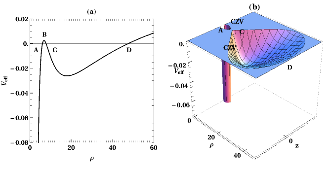
Figure 1: (a) The black curve shows the effective potential $V_{\textrm{eff}}$ for $\delta=2,~{}k=1,~{}E=0.97,~{}L_{z}=7.6,~{}z=0$ along the $\rho$ axis. The letters A, C, D indicate the positions of the $V_{\textrm{eff}}$ roots for $z=0$, while the black horizontal line shows the zero value of the $V_{\textrm{eff}}$ axis. The letter B indicates the position of a local maximum of the $V_{\textrm{eff}}$, which separates the plunging orbits from the bounded non-plunging. (b) The effective potential cut along the $V_{\textrm{eff}}=0$ plane. The A, C, D show the same as in (a) and the CZV corresponds to the curves of zero velocity.

II.2 Geodesic motion in the Zipoy Voorhees spacetime background

The equations of geodesic motion of a “test” particle of rest mass $\mu$ in a spacetime given by the metric $g_{\mu\nu}$ are produced by the Lagrangian function

$$L=\frac{1}{2}~{}\mu~{}g_{\mu\nu}~{}\dot{x}^{\mu}\dot{x}^{\nu}$$ (6)

where the dot denotes derivation with respect to proper time and the Greek indexes stand for spacetime coordinates. The Lagrangian (6) has a constant value $L=-\frac{\mu}{2}$ along a geodesic orbit, due to the $g_{\mu\nu}~{}\dot{x}^{\mu}\dot{x}^{\nu}=-1$ constraint.

Since the ZV spacetime is axisymmetric and stationary the corresponding momenta

$$p_{\nu}=\partial{L}/\partial{\dot{x}^{\nu}}$$ (7)

are conserved. These are the specific energy

$$E=-\frac{\partial L}{\partial\dot{t}}/\mu=-g_{tt}\dot{t},$$ (8)

and the specific azimuthal component of the angular momentum

$$L_{z}=\frac{\partial L}{\partial\dot{\varphi}}/\mu=g_{\phi\phi}\dot{\phi}~{}~{}.$$ (9)

For brevity, these two integrals are hereafter simply referred to as the energy $E$ and the angular momentum $L_{z}$.

The $z$ index refers to the cylindrical $(\rho,z)$ coordinate system used in all figures. The transformation equations from spheroidal prolate to cylindrical coordinates is

$$\rho=k\sqrt{(x^{2}-1)(1-y^{2})},~{}~{}~{}z=k~{}x~{}y~{}~{}.$$ (10)

The set of coordinates $(\rho,z)$ describes the meridian plane. Due to the two integrals of motion (8), (9) we can restrict our study to this plane. We just have to reexpress (8), (9) to get $\dot{t}$ and $\dot{\phi}$ as functions of $E$ and $L_{z}$, i.e.

$$\dot{t}=-E/g_{tt},~{}~{}\dot{\phi}=L_{z}/g_{\phi\phi}~{}~{},$$ (11)

and then substitute $\dot{t}$, $\dot{\phi}$ into the two remaining equations of motion. Then, from the original set of $4$ coupled second order ordinary differential equations (ODEs), we arrive at a set of $2$ coupled ODEs.

The motion on the meridian plane satisfies yet another constraint. If we use the transformation (10) on the metric (II.1), substitute (11) and replace the Lagrangian function with its constant value, we get

$$\frac{1}{2}(\dot{\rho}^{2}+\dot{z}^{2})+V_{\textrm{eff}}(\rho,z)=0,$$ (12)

where

$$V_{\textrm{eff}} = \frac{1}{2}Z\left(1+\frac{E^{2}}{g_{tt}}+\frac{L_{z}^{2}}{g_{\phi\phi}}\right),$$ (13)

$$Z = \left(\frac{r_{+}+r_{-}-2k}{r_{+}+r_{-}+2k}\right)^{\delta}\left(\frac{1}{2}+\frac{1}{4}\left(\frac{r_{+}}{r_{-}}+\frac{r_{-}}{r_{+}}\right)\right)^{-\delta^{2}},$$

$$r_{\pm} = \sqrt{\rho^{2}+(z\pm k)^{2}}.$$

The $V_{\textrm{eff}}$ corresponds to a Newtonian-like two-dimensional effective potential (Fig. 1). The roots ($V_{\textrm{eff}}=0$) of this effective potential (Fig. 1a) produce a curve on the meridian plane $(\rho,~{}z)$ called the curve of zero velocity (CZV) (Fig. 1b). This nomenclature follows from noting that whenever $V_{\textrm{eff}}=0$ the constraint (12) gives $\dot{\rho}=\dot{z}=0$, which means that whenever a geodesic orbit reaches the CZV the velocity component in the $\rho,~{}z$ plane becomes equal to zero.

On the meridian plane the CZV determines the set of initial conditions of geodesic orbits not escaping to infinity. These bounded orbits can either plunge to the central ZV compact object or revolve around it. In Fig. 1a the plunging orbits lie before point A, while the non-plunging orbits lie between the points C and D. In Fig. 1b the point A lies on the CZV containing all the plunging orbits, while C and D lie on the CZV containing the non-plunging orbits. This separation results from the fact that the local maximum of the effective potential at point B is greater than 0. If the angular momentum is reduced below $L_{z}=7.58$ for $\delta=2,~{}E=0.97$ (Fig. 1a), the maximum B drops below $0$ and a saddle point appears. This saddle point corresponds to an unstable periodic orbit similar to the unstable periodic orbit denoted with the letter “x” in Contop11 ; Contop12 , this notation is adopted in the present article as well.

In the integrable case $\delta=1$ (Schwarzschild metric) from such an unstable orbit “x” emanate the branches of the separatrix manifold, which separate the plunging from the non-plunging orbits. When the system is non-integrable, instead of the separatrix manifold, there are asymptotic manifolds emanating from the “x” orbit. “x” is formally called Lyapunov orbit (LO) Contop90 . Every orbit crossing the border defined by a LO “escapes”, which in our case means that every orbit which passes the LO while moving towards the central object, will plunge to the central object. On the other hand, for certain energy and angular momentum the “x” orbit changes its stability to indifferently stable and becomes the innermost stable circular orbit (ISCO).

In order to locate the ISCO, it is more convenient for the algebraic manipulation to use the potential $V=2~{}V_{\textrm{eff}}/Z$, instead of the effective potential (13). For the ISCO radius $x_{\textrm{ISCO}}$ the potential $V$ and its two first derivatives with respect to $x$ are equal to zero, i.e. $V|_{x_{\textrm{ISCO}}}=\frac{\partial V}{\partial x}|_{x_{\textrm{ISCO}}}=\frac{\partial^{2}V}{\partial x^{2}}|_{x_{\textrm{ISCO}}}=0$. Then we find

$$x_{\textrm{ISCO}} = 3\delta+\sqrt{5\delta^{2}-1},$$

$$E_{\textrm{ISCO}} = \sqrt{-g_{tt}|_{x_{\textrm{ISCO}}}\frac{x_{\textrm{ISCO}}-\delta}{x_{\textrm{ISCO}}-2\delta}},$$ (14)

$$L_{z_{\textrm{ISCO}}} = \sqrt{\frac{\rho^{2}}{g_{tt}|_{x_{\textrm{ISCO}}}}(1+\frac{E^{2}}{g_{tt}|_{x_{\textrm{ISCO}}}})}$$

for $\delta\geq 1/\sqrt{5}$. For $\delta<1/\sqrt{5}$, on the other hand the ZV spacetime ceases to have an ISCO. From a dynamical point of view, below this limit we may consider the ZV rather as a perturbation of the Minkowski ($\delta=0$) than of the Schwarschild ($\delta=1$) spacetime. The ISCO in the ZV spacetime was studied recently in Chowdhury12 , where the authors investigated the possible observational differences between the properties of accretion disks in the case of a ZV spacetime and a black hole spacetime.

II.3 Nonlinear Hamiltonian dynamics

By simply applying a Legendre transformation

$$H=p_{\mu}\dot{x}^{\mu}-L$$ (15)

on the Lagrangian function (6), we get the Hamiltonian function

$$H=\frac{1}{2~{}\mu}g^{\mu\nu}p_{\mu}p_{\nu}$$ (16)

where the momenta $p_{\mu}$ are given by (7) and $p^{\nu}=\mu\dot{x}^{\nu}$. It follows immediately that the ZV system is an autonomous system ($\frac{dH}{d\tau}=\frac{\partial H}{\partial\tau}=0$), thus the Hamiltonian function is an integral of motion and equal to $H=-\mu/2$ (because $g^{\mu\nu}p_{\mu}p_{\nu}=-\mu^{2}$)

As already mentioned in section II.2, the study of an axisymmetric and stationary system can be reduced to the meridian plane. Therefore, the system is reduced to a Hamiltonian system with two degrees of freedom. In the case of the Schwarzschild metric ($\delta=1$), spherical symmetry introduces an extra integral of motion, namely the total angular momentum. This integral is the reason why the Schwarzschild metric corresponds to an integrable system. In this case bounded non-plunging orbits oscillate in both degrees of freedom with two characteristic frequencies, denoted hereafter $\omega_{1}$ and $\omega_{2}$. The motion is restricted on a two-dimensional torus, called invariant torus. The type of motion on the torus depends on the ratio $\omega_{1}/\omega_{2}$. If the ratio is a rational number, the motion is periodic. The corresponding torus is called resonant and it hosts infinitely many periodic orbits with the same frequency ratio. On the other hand, if $\omega_{1}/\omega_{2}$ is irrational, the motion is called quasiperiodic. In that case, one single orbit densely covers the whole non-resonant torus.

In general, resonant and non-resonant tori align around a central periodic orbit forming the so-called tori foliation. If we move away from the central periodic orbit along any radial direction, we encounter tori with varying characteristic frequencies $\omega_{1},~{}\omega_{2}$. In fact, the ratio $\omega_{1}/\omega_{2}$ changes along the radial direction in the same way as the rational and the irrational numbers interchange along a real axis.

Now, if an integrable system (like Schwarzschild) is perturbed, the transition from integrability to non-integrability follows two basic theorems, namely the Kolmogorov-Arnold-Moser (KAM) theorem KAM and the Poincaré-Birkhoff theorem PoinBirk .

According to the KAM theorem, for small perturbations, most non-resonant invariant tori of the integrable system survive deformed in the perturbed system. The new deformed tori are called KAM tori.

On the other hand, according to the Poincaré-Birkhoff theorem, from the infinitely many periodic orbits on a resonant torus of the integrable system only an even number survive in the perturbed system. Half of these surviving periodic orbits are stable and the other half unstable.

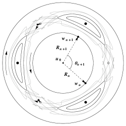
Figure 2: A schematic representation of a surface of section of a non-integrable Hamiltonian system of two degrees of freedom. The figure shows a Birkhoff chain at the resonance $1/3$ between two KAM curves (homocentric cyclic curves around the central periodic point $\mathbf{u}_{0}$). The Birkhoff chains consists of 3 unstable points (open circles) and 3 stable points (filled circles). An island of stability is formed around each of the 3 stable points (elliptic curves). From the unstable points emanate asymptotic curves (gray curves). The arrowheads on the asymptotic curves indicate the stable and the unstable branch. The curved arrows indicate the flow in the phase space. The points $\mathbf{w}_{n},~{}\mathbf{w}_{n+1}$ indicate two successive crossings of the quasiperiodic orbit forming the KAM curve. $\theta_{n+1}$ is the angle between the position vectors $\mathbf{R}_{n},~{}\mathbf{R}_{n+1}$ (with respect to $\mathbf{u}_{0}$) of the points $\mathbf{w}_{n},~{}\mathbf{w}_{n+1}$ respectively.

The structure of the phase space is revealed conventionally by the use of a 2-dimensional Poincaré surface of section. On a surface of section, the invariant tori correspond to closed curves, such curves are shown in Fig. 2 (schematic). For weakly perturbed systems the KAM curves on the surface of section are closed invariant curves around a stable fixed point in the center (like $\mathbf{u}_{0}$ in Fig. 2). This structure is hereafter called the main island of stability.

However, the details of the surface of section of a non-integrable Hamiltonian system close to resonances are quite different from those of integrable systems. The stable surviving periodic orbits are depicted as stable points on a surface of section (filled circles in Fig. 2) and these points are surrounded by other regular orbits forming the secondary islands of stability (Fig. 2). Between these islands lie unstable points (open circles in Fig. 2), which correspond to unstable periodic orbits. From the unstable periodic orbits emanate their asymptotic manifolds, yielding asymptotic curves on the surface of section (gray curves of Fig. 2). There are two types of asymptotic curves: stable and unstable. A stable (unstable) asymptotic manifold cannot cross itself or other stable (unstable) asymptotic manifolds. Initial conditions on a stable (unstable) manifold tend asymptotically to the periodic orbit in the inverse (direct) flow of the time parameter. The latter property of asymptotic manifolds, combined with the non-crossing property produce on the surface of section oscillations of the manifolds, causing the so-called homoclinic “chaos” effect. Due to this, if we start with initial conditions within the domain crossed by manifolds, their subsequents give the impression of scattered points, which are a signature of chaotic motion on a surface of section.

Besides the use of a surface of section, another tool to study non-integrable systems is the rotation number $\nu_{\theta}$. The rotation number has been proved to be an efficient indicator of chaos Laskar93 ; Contop97 ; Voglis98 (see Contop02 for review). A simple way to evaluate the rotation number is the following. First we identify the central periodic orbit ($\mathbf{u}_{0}$ in Fig. 2) of the main island of stability. Then, we define the position vector

$$\mathbf{R}_{n}=\mathbf{w}_{n}-\mathbf{u}_{0}$$ (17)

of the n-th crossing $\mathbf{w}_{n}$ of the orbit through a surface of section with respect to the central periodic orbit $\mathbf{u}_{0}$ (dashed vectors in Fig. 2). We then find the angle between two successive vectors $\theta_{n+1}\equiv angle(\mathbf{R}_{n+1},\mathbf{R}_{n})$ (called the rotation angle) and we evaluate the rotation number

$$\nu_{\theta}=\frac{1}{2\pi N}\sum_{n=1}^{N}\theta_{n}~{}~{}.$$ (18)

In the limit $N\rightarrow\infty$, the rotation number corresponds to the frequency ratio $\omega_{1}/\omega_{2}$.

If we plot the rotation number as a function of the distance of initial conditions from the central periodic orbit $\mathbf{u}_{0}$ of the main island of stability along a particular direction we obtain the so-called rotation curve. For integrable systems, like the Schwarzschild metric, the rotation curve is a smooth and strictly monotonic function. When the system is perturbed, the rotation curve ceases to be smooth, and it is only approximately monotonic. In fact, the imprints of chaos are found in the rotation curve, as demonstrated by several examples in section III.

III Numerical results

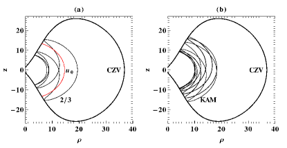
Figure 3: The projections of geodesic orbits on the meridian plane ($(z,\rho)$) for $\delta=2,~{}k=1$, $E=0.95$ and $L_{z}=3$. (a) The simple periodic orbit $\mathbf{u}_{0}$ (red/gray curve) and the $2/3$ periodic orbit (black curve). (b) A quasiperiodic (KAM) orbit. In both panels, the boundary of motion on the meridian plane is determined by the CZV (thick curve).

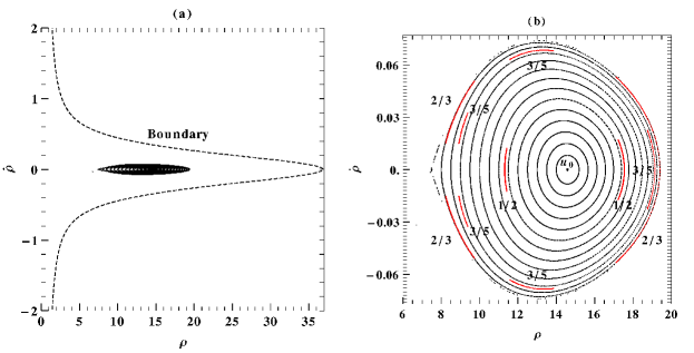
Figure 4: (a) The surface of section $z=0$ ($\dot{z}>0$) for $\delta=2$, $E=0.95$ and $L_{z}=3$. The dashed black curve determines the boundary of the bounded orbits. The closed curves are KAM curves of the main island of stability, while the empty phase space between the the main island of stability and the boundary curve is occupied by plunging orbits. (b) A magnification of the main island of stability. The point $\mathbf{u}_{0}$ is the central fixed point. Various islands of stability forming Birkhoff chains are shown, labeled by their corresponding rotation numbers.

Previous numerical investigations of the ZV system Sota96 ; Brink08 have led to a conjecture that this system is integrable. This led to attempts of finding the missing integral of motion Brink08 ; KrugMat11 . In KrugMat11 , however, the authors proved the non-existence of a broad category of integrals of motion for the $\delta=2$ case. The parameter $\delta=2$ was used also in Brink08 , where the values $E=0.95$, $L_{z}=3$ and $k=1$ ($\delta=M$) were chosen for the numerical examples. The same values are applied in the subsequent section III.1 in order to provide a straight forward comparison with previous studies, while cases for different values of $\delta$ are presented as well.

III.1 Cases with $\delta>1$

The periodic orbits on the meridian plane are bounded by the CZV (section II.2). Two examples of periodic orbits projected on the meridian plane are given in Fig. 3a. The first is the simple periodic orbit $\mathbf{u}_{0}$ (red/gray curve in Fig. 3a), which bounces along an arc between two points of the CZV (thick curves in Fig. 3). The second is a stable periodic orbit of the resonance $2/3$ (black curve in Fig. 3a), which bounces also between points of the CZV but follows a more complex path. The path is even more complicated in the case of a quasiperiodic orbit (Fig. 3b), because the quasiperiodic orbits cover densely their hosting KAM tori (section II.3).

Fig. 4, now, shows the surface of section $z=0$ ($\dot{z}>0$) corresponding to orbits like those of Fig. 3. The orbits shown on the surface of section plane ($\rho,~{}\dot{\rho}$) are in general non-equatorial. The bounded orbits lie inside the boundary curve $\dot{\rho}=\pm\sqrt{-2~{}V_{\textrm{eff}}(z=0)}$ (dashed curve in Fig. 4a). Most of them are plunging orbits and only a small main island of stability of non-plunging orbits appears in the center of Fig. 4a.

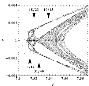
Figure 5: Detail of the left tip of the main island of stability shown in Fig. 4b. The arrows are showing the position of the islands of stability of the resonances $11/14,~{}18/23,~{}31/40,~{}10/13$ along the $\dot{\rho}=0$ line.

At first glance the magnified surface of section in Fig. 4b seems to be quite regular, with no prominent signs of chaos. However, at the resonances $1/2,~{}3/5,~{}2/3$ thin islands of stability appear. These indicate the existence of Birkhoff chains and, therefore, of chaos. In fact, if we zoom at the left tip of the main island of stability we already get a typical picture of a chaotic layer (Fig. 5). In Fig. 5 the scattered points define chaotic regions, while the continuous curves define the limits of regular domains. However, the separation between chaotic and regular regions is not so clear. For example, the islands of stability belonging to the resonances $11/14,~{}18/23,~{}31/40$ are embedded in prominent chaotic layers (Fig. 5).

Most of the chaotic orbits of Fig. 5 are plunging orbits which, due to the phenomenon of stickiness ContopHars , remain for a long time close to regular non-plunging orbits, before crossing the LO and plunge. The LO lies approximatively at the edge tip formed at the left of the main island of stability of Fig. 5. In fact the region between the main island of stability and the boundary curve (Fig. 4a) is covered by chaotic plunging orbits. The chaotic orbits stick around islands of higher multiplicity, e.g. the islands of stability $11/14,~{}18/23,~{}31/40$ (Fig. 5), before they plunge. The multiplicity is equal to the denominator of the prime number ratio corresponding to the rotation number.

Figure 6: The rotation number as a function of the initial conditions lying on the $\dot{\rho}=0$ line of Fig. 5. Prominent islands of stability are labeled by the respective rational value of $\nu_{\theta}$.

The rotation curve along the $\dot{\rho}=0$ line of Fig. 5 is shown in Fig. 6. The regions dominated by regular motion are represented by relatively smooth segments of the curve, while the chaotic regions are recognized by various distinct parts where the rotation curve develops fluctuations. At certain smooth segments of the rotation curve, the rotation number is constant. These segments appear like “plateaus” of the rotation curve. Distinct plateaus correspond to islands of stability of distinct resonances in Fig. 5. In Fig. 6 the most prominent plateaus are labeled by the value of the rotation number at each respective resonance.

Figure 7: The rotation curve along the line $\dot{\rho}=0$ corresponding to the Fig. 4b. The embedded figure shows a detail of the curve at the $2/3$ resonance.

In fact, the computation of the rotation curve is an efficient way to look for initial conditions leading to Birkhoff islands of stability, since the latter can be located by the plateaus of the rotation curve. This method is particularly useful in the location of tiny, or narrow islands, such us in Fig. 4b. In this case, by scanning along the line $\dot{\rho}=0$ the corresponding rotation curve (Fig. 6) seems to be rather smooth (excluding the last part corresponding to the chaotic layer surrounding the main island of stability). However, a detailed scan reveals a number of lower multiplicity resonances (e.g. the resonances $1/2,~{}2/3,~{}3/5$ shown in Fig. 4). Lower multiplicity resonant structures (like islands of stability) are more prominent than higher multiplicity ones (as e.g. the resonance $10/13$ shown in Fig. 5). By focusing on the lower multiplicity resonances the anticipated plateaus of the islands of stability clearly appear on the rotation curve. An example is shown for the plateau of the conspicuous $2/3$ island of stability in the embedded panel of Fig. 7.

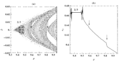
Figure 8: (a) A detail of the $z=0$ ($\dot{z}>0$) surface of section for $\delta=3$, $E=0.98$, $L_{z}=7$ and $k=1$. An island of stability belonging to the $2/3$ resonance is shown embedded in a chaotic layer, while the arrows indicate the position of the unstable periodic points of other Birkhoff chains. (b) The rotation curve along the line $\dot{\rho}=0$ corresponding to Fig. 8a. The plateau of the $2/3$ is denoted and the arrows denote the behavior of the rotation curve when it crosses unstable periodic points.

If we change the value of the $\delta$ parameter to $\delta=3$ the structure of the phase space does not change significantly. Near the outer boundary of the main island there is a sticky chaotic layer of plunging orbits (Fig. 8a) and Birkhoff chains appear inside the main island of stability. The corresponding rotation curve in Fig. 8b shows large variations whenever it crosses initial conditions belonging to chaotic orbits. Also, the rotation curve takes the form of a plateau when crossing resonant islands of stability, and it changes abruptly when crossing the unstable periodic points of relatively small resonances (arrows in Fig. 8b). Thus, in the case of $\delta=3$ as well both detecting methods, i.e. the surface of section and the rotation number, indicate that the ZV metric is not integrable.

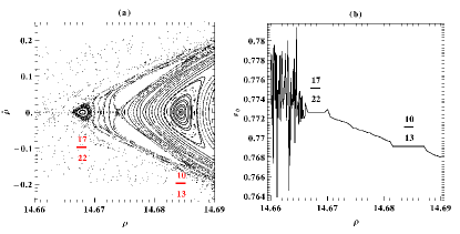
Figure 9: (a) A detail of the $z=0$ ($\dot{z}>0$) surface of section for $\delta=4$, $E=0.95$, $L_{z}=3$ and $k=1$. (b) The rotation curve along the line $\dot{\rho}=0$ corresponding to Fig. 9a.

If we further increase the value of $\delta$, the overall picture of the phase space is qualitatively similar to the cases already presented. However, what changes is the position of the unstable point “x” (section II.2), which moves further away from the central anomaly $\rho=z=0$. This is expected, since the position of the ISCO moves away as well (first equation of eqs. (II.2)). Thus, for increasing $\delta$ the main island of stability moves all together to larger distances $\rho$. For example, Fig. 9 shows a detail of the phase space for $\delta=4$, $E=0.95$, $L_{z}=3$, where the whole island structure has been shifted further away from $\rho=z=0$ with respect to Figs. 5, 6, 8.

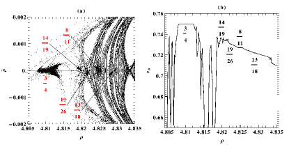
Figure 10: (a) A detail of the $z=0$ ($\dot{z}>0$) surface of section for $\delta=3/2$, $E=0.98$, $L_{z}=5.7$ and $k=1$. (b) The rotation curve along the line $\dot{\rho}=0$ corresponding to Fig. 10a.

In all previous cases the value of $\delta$ was a natural number. However, the structure of the phase space seems not to change even if $\delta$ is a positive real (not integer) number. For instance, if $\delta=3/2$, then we find again a chaotic layer around the main island of stability (Fig. 10), and all the complexity seen in the previous examples as well. In particular, islands of stability are either embedded in a prominent chaotic layer or enveloped between KAM curves (Fig. 10a). The resonances corresponding to these islands are found in Fig. 10b by the use of the rotation number. Fig. 10b is a good example to note again that lower multiplicity islands of stability are more prominent than the higher multiplicity ones. This fact is the reason why we expect Apostolatos09 ; Lukes10 that the lower multiplicity islands of stability are good candidates for detecting non-Kerr compact objects by the analysis of gravitational waves coming from EMRIs, even if the inspiraling smaller compact object might cross infinite resonances in a bumpy black hole spacetime background during its inspiral.

III.2 Cases with $\delta<1$

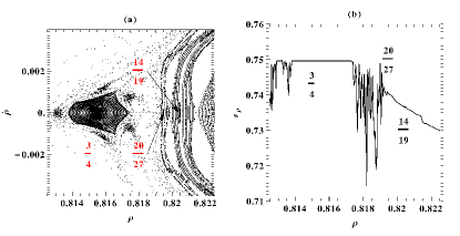
Figure 11: (a) A detail of the $z=0$ ($\dot{z}>0$) surface of section for $\delta=1/2$, $E=0.99$, $L_{z}=1.8$ and $k=1$. (b) The rotation curve along the line $\dot{\rho}=0$ corresponding to Fig. 11a.

When $\delta<1$, the ZV spacetime corresponds to a more prolate central object than the respective Schwarzschild black hole. Nevertheless, for the prolate case $\delta=1/2$ the structure of the phase space is similar to the oblate cases examined in section III.1. There is a main island of stability, and around it a chaotic sea of plunging orbits. In particular, the detail of the surface of section $z=0$ ($\dot{z}>0$) (Fig. 11a) presents a similar phase space structure near the sticky chaotic layer around the main island of stability as in the oblate cases shown in section III.1. Thus, we find again the $3/4$ Birkhoff chain, from which we can see clearly one of the respective islands of stability embedded in the chaotic sea. Islands of higher multiplicity lie near the border of the chaotic layer and of the main island of stability. Thus, it seems that the ZV system has a similar dynamical behavior independently of whether the corresponding central object is more oblate or prolate than a Schwarzschild black hole.

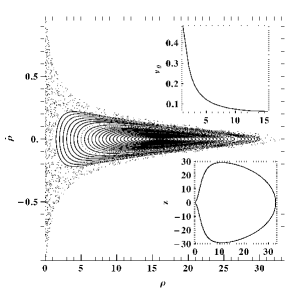
Figure 12: The $z=0$ ($\dot{z}>0$) surface of section for $\delta=1/3$, $E=0.99$, $L_{z}=0.4$ and $k=1$. In the lower right embedded figure is shown the corresponding CZV. In the upper right embedded figure is shown the rotation curve along the $\dot{\rho}=0$ for the segment corresponding to the main island of stability.

However, if we reduce further the parameter $\delta$, for instance to $\delta=1/3$, then the dynamical behavior changes significantly. This change is expected for $\delta<1/\sqrt{5}$, because as noted in the last paragraph of section II.2 the ZV spacetime loses a property, namely the existence of an ISCO, which is a characteristic of a black hole spacetime. In Fig. 12 the surface of section shows a main island of stability surrounded by a chaotic sea. Due to the fact that the CZV is a closed curve (bottom right embedded panel in Fig. 12), the orbits of the chaotic sea cannot plunge towards the central anomaly. As a result, even if the chaotic sea is prominent in size, no strong chaotic regions can be seen inside the main island of stability. This fact is confirmed both by the surface of section and by the rotation curve (main panel and right up panel in Fig. 12 respectively). Thus, the structure of the main island of stability seems not to change significantly for $\delta<1/\sqrt{5}$ (compare the surface of section and the rotation curve in Fig. 12 with that in Figs. 4, 7 respectively).

IV Conclusions and Discussion

It has been shown by clear numerical examples that the ZV metric corresponds in general to a non-integrable system, contrary to the results of previous works Sota96 ; Brink08 . The only known ZV spacetimes that correspond to integrable systems, are the Minkowski spacetime ($\delta=0$) and the Schwarzschild spacetime ($\delta=1$). In order to find imprints of the ZV non-integrability the methods of the surface of section and of the rotation number were employed.

In fact, in cases like the ZV system, we can only guess where to zoom on a surface of section to discover chaotic layers or other imprints of chaos. However, in such cases of nearly integrable Hamiltonian systems, chaos is strongly correlated with the remnants of the destroyed resonance tori (section II.3). Therefore, a tool, like the rotation number, which detects resonances is very useful.

Moreover, the rotation number is a reliable indicator of chaos. Thus, even if we do not use a surface of section or another method for detecting chaos, the rotation curves themselves are sufficient to show that chaos exists. This is interesting also from an observational point of view, because the rotation number is the ratio of the two main frequencies of a non-plunging geodesic orbit. Therefore, the rotation number is an adequate tool for detecting phenomena associated with chaos in gravitational wave signals. This has been already studied in Apostolatos09 ; Lukes10 , where the rotation number was used in order to detect deviations from the Kerr metric in a case of an EMRI into a bumpy black hole spacetime background.

It has been shown that the ZV spacetime has a similar dynamical behavior in all cases, i.e. independently of whether the spacetime corresponds to a more oblate or prolate central compact object, as long as $\delta\geq 1/\sqrt{5}$. In particular, all the orbits belonging to the chaotic sea which surrounds the main island of stability are plunging. When, $0<\delta<1/\sqrt{5}$ then the ISCO disappears and the orbits of the chaotic sea cease to be plunging. Thus, $\delta=1/\sqrt{5}$ is a marginal value, where the ZV metric family changes its behavior.

Finally, the study of bumpy black holes ISCOs has an interesting aspect regarding spin measurements of Kerr black holes. If we suppose that ZV is describing the spacetime around a compact object, then in the interval $1/\sqrt{5}<\delta<1$ we get ISCO positions that correspond to the Kerr black hole ones. This fact implies that if we evaluate the central compact object spin by calculating the ISCO position like in McClintock11 without having tested the Kerr hypothesis first, then these measurements might be misleading.

Appendix A Numerical accuracy

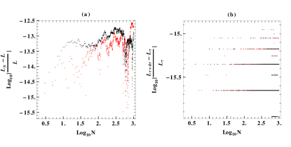
Figure 13: (a) The relative error $|\frac{L_{N}-L}{L}|$ of the Lagrangian function $L$, which is a constant, as evaluated at the $N$th surface of section. (b) The relative error $|\frac{L_{\tau+d\tau}-L_{\tau}}{L_{\tau}}|$ between the Lagrangian function two consecutive integration steps at the $N$th surface of section. The red (gray) points corresponds to a chaotic orbit with initial condition $\dot{\rho}=z=0,~{}\rho=7.518$, while the black to a regular orbit with initial condition $\dot{\rho}=z=0,~{}\rho=7.548$. Both initial conditions lie on the surface of section shown in Fig. 5.

For integrating the geodesic orbits in the ZV system the 5th order Cash-Karp Runge-Kutta was applied with a step size controller developed by the author. The controller’s function is to keep the relative error $|\frac{L_{\tau+d\tau}-L_{\tau}}{L_{\tau}}|$ of the evaluated Lagrangian $L_{\tau}$, $L_{\tau+d\tau}$ functions between two consecutive integration steps $\tau$, $\tau+d\tau$ below a tolerance value. Even if such a control can secure the accuracy between two consecutive integration steps, it cannot guarantee the accuracy of the overall calculation. The integration accuracy is checked by the relative error $|\frac{L_{\tau}-L}{L}|$, where the evaluated Lagrangian function $L_{\tau}$ is compared with the theoretical one $L$.

The overall time evolution of the relative error $|\frac{L_{N}-L}{L}|$ at the Nth surface of section crossing is shown in Fig. 13a for a regular orbit (black dots) and for a chaotic orbit (red/gray points). The evolution of the relative error $|\frac{L_{\tau+d\tau}-L_{\tau}}{L_{\tau}}|$ for the same orbits is shown in Fig. 13b. Although the relative error at consecutive steps appears rather small, the overall error shows that both chaotic and regular orbits exhibit slow numerical drift. However, in both cases this drift is very small compared to the scale of studied phenomena.

References

- (1) P. Amaro-Seoane, S. Aoudia, S. Babak, et al., arXiv:1201.3621
- (2) P. Amaro-Seoane, S. Aoudia, S. Babak, et al., Class. Quantum Gravity 29, 124016 (2012)
- (3) F. D. Ryan, Phys. Rev. D 52, 5707 (1995); 56, 1845 (1997)
- (4) C. Li and G. Lovelace, Phys. Rev. D 77, 064022 (2008)
- (5) G. Pappas and T. A. Apostolatos, Phys. Rev. Lett. 108, 231104 (2012)
- (6) N. A. Collins and S. A. Hughes, Phys. Rev. D 69, 124022 (2004)
- (7) S. J. Vigeland, Phys. Rev. D, 82 104041 (2010)
- (8) K. Glampedakis and S. Babak, Class. Quantum Gravity 23, 4167 (2006)
- (9) E. Barausse, L. Rezzolla, D. Petroff and M. Ansorg, Phys. Rev. D 75, 064026 (2007)
- (10) J. R. Gair, C. Li and I. Mandel, Phys. Rev. D 77, 024035 (2008)
- (11) T. A. Apostolatos, G. Lukes-Gerakopoulos and G. Contopoulos, Phys. Rev. Lett. 103, 111101 (2009)
- (12) S. J. Vigeland and S. A. Hughes, Phys. Rev. D 81, 024030 (2010)
- (13) G. Lukes-Gerakopoulos, T. A. Apostolatos and G. Contopoulos, Phys. Rev. D 81, 124005 (2010)
- (14) S. J Vigeland, N. Yunes and L. C. Stein, Phys. Rev. D 83, 104027 (2011)
- (15) J. Gair and N. Yunes, Phys. Rev. D 84, 064016 (2011)
- (16) T. Johannsen and D. Psaltis, Astrophys. J. 716, 187 (2010); 718, 446 (2010); 726, 11 (2011); 745, 1 (2011); Adv. Space Res., 47, 528 (2011); arXiv:1202.6069
- (17) C. Bambi and E. Barausse, Astrophys. J. 731, 121 (2011)
- (18) C. Bambi, Phys. Rev. D 83, 103003 (2011); 85, 043001 (2012); 85, 043002 (2012)
- (19) G. Pappas, Mon. Not. R. Astron. Soc. 422, 2581 (2012)
- (20) C. Bambi, Mod. Phys. Lett. A 26, 2453 (2011)
- (21) T. Johannsen, Adv. Astron. (2012)
- (22) G. Contopoulos, G. Lukes-Gerakopoulos and T. A. Apostolatos, Int. J. Bifurc. Chaos 21, 2261 (2011)
- (23) G. Contopoulos, M. Harsoula and G. Lukes-Gerakopoulos, arXiv:1203.1010
- (24) B. Carter, Phys. Rev. 174, 1559
- (25) C. M. Will, Phys. Rev. Lett. 102, 061101 (2009)
- (26) C. Markakis, arXiv:1202.5228
- (27) D. M. Zipoy, J. Math. Phys. 7, 1137 (1966)
- (28) B. H. Voorhees, Phys. Rev. D 2, 2119 (1970)
- (29) F. P. Esposito and L. Witten, Phys. Lett. B 58, 357 (1975)
- (30) Y. Sota, S. Suzuki K.-I. Maeda, Class. Quantum Gravity 13, 1241 (1996)
- (31) J. Brink, Phys. Rev. D 78, 102002 (2008)
- (32) B. S. Kruglikov and V. S. Matveev, arXiv:1111.4690
- (33) J. Laskar, Celest. Mech. Dyn. Astron. 56, 191 (1993)
- (34) G. Contopoulos and N. Voglis, Astron. Astrophys. 317, 73 (1997)
- (35) N. Voglis and C. Efthymiopoulos, J. Phys. A 31, 2913 (1998)
- (36) L. Herrera, F. M. Paiva and N. O. Santos, J. Math. Phys. 40, 4064 (1999)
- (37) H. Kodama and W. Hikida, Class. Quantum Gravity 20, 5121 (2003)
- (38) D. Papadopoulos, B. Stewart and L. Witten, Phys. Rev. D 24, 320 (1981)
- (39) G. Contopoulos, Astron. Astrophys. 231, 41-55 (1990)
- (40) A. N. Chowdhury, M. Patil, D. Malafarina & P. S. Joshi, Phys. Rev. D 85, 104031 (2012)
- (41) A. N. Kolmogorov, Dokl. Akad. Nauk SSSR 98, 527 (1954); V. I. Arnold, Russ. Math. Surv. 18, 13 (1963); J. Moser, Nachr. Akad. Wiss. Göttingen Math. Phys. K1 II 1 (1962)
- (42) H. Poincaré, Rend. Circ. Mat. Palermo 33, 375 (1912); G. D Birkhoff, Trans. Am. Math. Soc. 14, 14 (1913)
- (43) G. Contopoulos, “Order and chaos in dynamical astronomy” (Springer, Berlin, 2002)
- (44) G. Contopoulos and M. Harsoula, Int. J. Bifurc. Chaos 18, 2929 (2008); 20, 2005 (2010)
- (45) J. E. McClintock, R. Narayan, S. W. Davis, et al., Class. Quantum Gravity 28, 114009 (2011)