Polytropic scalar field models of dark energy

Abstract

Abstract

In this work we investigate the polytropic gas dark energy model in the non flat universe. We first calculate the evolution of EoS parameter of the model as well as the cosmological evolution of Hubble parameter in the context of polytropic gas dark energy model. Then we reconstruct the dynamics and the potential of the tachyon and K-essence scalar field models according to the evolutionary behavior of polytropic gas model.

I Introduction

Nowadays our belief is that the current universe is in accelerating expansion. The results of cosmological experiments: SNe Ia c1 , WMAP c2 , SDSS c3 and X-ray c4 , have provided the main evidences for this cosmic acceleration. In the framework of standard cosmology, a new energy with negative pressure, namely dark energy (DE), is needed to explain this acceleration. The cosmological constant with the time - independent equation of state $w_{\Lambda}=-1$ is the earliest and simplest candidate of dark energy. Although the cosmological constant is consistent with observational data, but from the theoretical viewpoint is faces with the fine-tuning and cosmic coincidence problems fin . In addition to cosmological constant, the other dynamical dark energy models with time-varying equation of state have been suggested to explain the cosmic acceleration. Recent SNe Ia observational data show that the dynamical dark energy models have a better fit compare with cosmological constant c44 . The scalar field models such as quintessence c5 , phantom c6 , quintom c7 , K-essence c8 , tachyon c9 and dilaton c10 together with interacting dark energy models such as holographic c11 and agegraphic c12 models are the examples of dynamical dark energy models.
The holographic dark energy model comes from the holographic principle of quantum gravity c13 and the agegraphic model has been proposed based on the uncertainty relation of quantum mechanics together with general relativity c14 .
In this work, we focus on the polytropic gas model as a dark energy model to explain the cosmic acceleration. In stellar astrophysics, the polytropic gas model can explain the equation of state of degenerate white dwarfs, neutron stars and also the equation of state of main sequence stars c19 . The idea of dark energy with polytropic gas equation of state has been investigated by U. Mukhopadhyay and S. Ray in cosmology ray05 . The polytropic gas is a phenomenological model of dark energy. In a phenomenological model, the pressure $p$ is a function of energy density $\rho$, i.e., $p=-\rho-f(\rho)$ c177 . For $f(\rho)=0$, the equation of state of phenomenological models can cross $w=-1$, i.e., the cosmological constant model. Nojiri, et al. investigated four types singularities for some illustrative examples of phenomenological models c177 . The polytropic gas model has a type III. singularity in which the singularity takes place at a characteristic scale factor $a_{s}$.
Recently, Karami et al. investigated the interaction between dark energy and dark matter in polytropic gas scenario, the phantom behavior of polytropic gas, reconstruction of $f(T)$- gravity from the polytropic gas and the correspondence between polytropic gas and agegraphic dark energy model c17 ; c18 ; karam20 . The cosmological implications of polytropic gas dark energy model is also discussed in malek1 . The evolution of deceleration parameter in the context of polytropic gas dark energy model represents the decelerated expansion at the early universe and accelerated phase later as expected. The polytropic gas model has also been studied from the viewpoint of statefinder analysis in malek_state .
On the other hands, as we know, the scalar field models are the effective description of an underlying theory of dark energy. Scalar fields naturally arise in particle physics including supersymmetric field theories and string/M theory. The scalar field can reveal the dynamic and the nature of dark energy. However, the fundamental theories such as string/M theory do not predict their potential $V(\phi)$ uniquely. Consequently, it is meaningful to reconstruct the potential of dark energy model so that these scalar fields can describe the evolutionary behavior of dark energy model possessing some significant features of the quantum gravity theory, such as holographic and agegraphic dark energy models. In this direction, many works have been done scalar . In this paper we reconstruct the dynamics and the potential of tachyon and the K-essence scalar fields model according to the evolution of polytropic gas model.

II FRW cosmology and polytropic gas dark energy

Let us start with non-flat Friedmann-Robertson-Walker (FRW) universe containing dark energy and dark matter, the corresponding Friedmann equation is as follows

$$H^{2}+\frac{k}{a^{2}}=\frac{1}{3M_{p}^{2}}(\rho_{m}+\rho_{d})$$ (1)

where $H$ is the Hubble parameter, $M_{p}$ is the reduced Plank mass and $k=1,0,-1$ is a curvature parameter corresponding to a closed, flat and open universe, respectively. $\rho_{m}$ and $\rho_{\Lambda}$ are the energy density of dark matter and dark energy, respectively. Recent observations support a closed universe with a tiny positive small curvature $\Omega_{k}=\simeq 0.02$ c20 .
In the case of dimensionless energy densities

$$\Omega_{m}=\frac{\rho_{m}}{\rho_{c}}=\frac{\rho_{m}}{3M_{p}^{2}H^{2}},~{}~{}~{}\\ \Omega_{d}=\frac{\rho_{d}}{\rho_{c}}=\frac{\rho_{d}}{3M_{p}^{2}H^{2}}~{}~{}\\ \Omega_{k}=\frac{k}{a^{2}H^{2}},$$ (2)

the Friedmann equation (1) can be written as

$$\Omega_{m}+\Omega_{d}=1+\Omega_{k}.$$ (3)

The conservation equations for dark matter and dark energy are given by

$$\dot{\rho_{m}}+3H\rho_{m}=0,$$ (4)

$$\dot{\rho_{\Lambda}}+3H(\rho_{d}+p_{d})=0,$$ (5)

The equation of state (EoS) of polytropic gas is given by

$$p_{d}=K\rho_{d}^{1+\frac{1}{n}},$$ (6)

where $K$ and $n$ are constants of the model c19 . Inserting Eq.(6) in (5) and integrating obtains the energy density of polytropic gas dark energy as

$$\rho_{d}=\left(\frac{1}{Ba^{3/n}-K}\right)^{n},$$ (7)

where $B$ is the integration constant and $a$ is the scale factor. For $Ba^{3/n}>K$ the energy density of polytropic gas is positive for any odd and event number of $n$. But in the case of $Ba^{3/n}<K$ the energy density is positive only for even numbers. The phantom behavior of interacting polytropic gas dark energy has been calculated in c17 . The phenomenological equation of state such as chaplygin gas and polytropic gas models usually suffers from the singularity problem in which the energy density tends to infinity. The singularity of dark energy models has been discussed in noji12 . In the case of $Ba^{3/n}=K$, we have $\rho_{d}\rightarrow\infty$ and the polytropic gas has a finite-time singularity at $a_{c}=(K/B)^{n/3}$. This type of singularity has been named by type III singularity noji12 .
Tacking the time derivative of (7) with respect to time obtains

$$\dot{\rho_{d}}=-3BHa^{\frac{3}{n}}\rho_{d}^{1+\frac{1}{n}}$$ (8)

Substituting (8)in conservation equation of dark energy component (5) and using (7), $p_{d}=w_{d}\rho_{d}$, in (5) we obtain the EoS parameter of polytropic gas dark energy model as

$$w_{d}=-1-\frac{a^{\frac{3}{n}}}{c-a^{\frac{3}{n}}}$$ (9)

where $c=K/B$. Here one can see that the polytropic gas model can cross the phantom line, i.e. $w_{d}=-1$, when $c>a^{3/n}$. Also at the early time ($a\rightarrow 0$), the polytropic gas mimics the cosmological constant, i.e. $w_{d}\rightarrow-1$.
In figure (1), the evolution of EoS parameter $w_{d}$ is plotted as a function of redshift parameter $z$. Note that the redshift parameter is related to scale factor by $a=1/(1+z)$. Here we conclude that the polytropic gas model for the selected model parameter:$c=2$ and even numbers: {$n=2,4,6$} behaves as a phantom dark energy as indicated in left panel. Also in the right panel the phantom regime can be obtained for different illustrative values {$c=2,3,4$} and even number $n=2$.
From (7), we see that the polytropic gas has a singularity at $a_{s}=c^{n/3}$. For $c<1$, this singularity takes place at $a_{s}<1$ (past). For $c=1$ the singularity occurs at the present time $a_{s}=1$ and in the case of $c>1$ it occurs at future, i.e. $a_{s}>1$. In figure (2) we show the singularity of polytropic gas model for different values of $c$. In upper left panel we choose $c=2$. In this case the singularity of the model tacks place at future ($a_{s}=1.58$). In upper right panel $c=1$ and the singularity occurs at the present time $a_{s}=1$. Eventually at the lower panel, for $c=0.4$, the singularity occurs at the past time $a_{s}=0.57$. One of the advantage of polytropic gas model is that this model can behaves as a phantom dark energy without a need to interaction between dark matter and dark energy. From figure (1), we see the that the phantom regime ($w_{d}<-1$) for polytropic gas as indicated by (9). But the other theoretical models of dark energy such as holographic and agegraphic can not enter the phantom regime without interaction term, for example see cai22 ; setare22 . From (9), we also see that for the condition of $c<a^{3/n}$, the polytropic gas can behave as a quintessence model,i.e., $-1<w_{d}<0$. The problem of phenomenological models such as polytropic gas model is that, because of singularity at $a_{s}$, the cosmology for these models can be defined only in the interval $0<a<a_{s}$, i.e., from the Big Bang epoch to the singularity epoch at $a_{s}$. In other word, the polytropic gas model can describe the acceleration of the universe from the Big Bang epoch up to singularity epoch at the scale factor $a_{s}$. In the next section we reconstruct the potential and the dynamics of tachyon scalar field according to the evolution of phantom polytropic gas dark energy.
We now obtain the Hubble parameter in the context of polytropic dark energy model. From the conservation equations (4), (5) and using the dimensionless energy densities in (2), we have

$$\rho_{m}=\rho_{m0}a^{-3}$$ (10)

$$\rho_{d}=\rho_{d0}a^{-3[1+w_{d}(a)]}$$ (11)

Inserting (10,11) in Friedmann equation (1) and using the dimensionless energy densities (2), we obtain the Hubble parameter as

$$H(a)=H_{0}\sqrt{\Omega_{m0}a^{-3}+\Omega_{d0}a^{-3[1+w_{d}(a)]}-\Omega_{k0}a^{-2}}$$ (12)

where $w_{d}(a)$ is given by (9).
In figure (3), we plot the evolution of dimensionless Hubble parameter, $E(a)=H(a)/H_{0}$, for polytropic gas model. In left panel, we fix $c$ and vary the parameter $n$. The smaller value the parameter $n$ is taken, the bigger the Hubble parameter expansion rate E(a) can reach. In right panel, by fixing $n$, we vary the parameter $c$. The dimensionless Hubble parameter E(a) is bigger for larger value of $c$. One can explicitly see that both the model parameters $n$ and $c$ can impact the expansion of the universe.

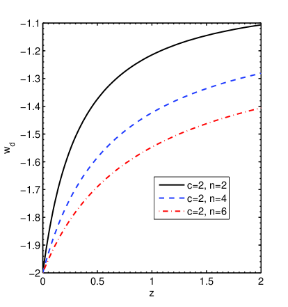
Figure 1: The EoS parameter of polytropic gas model for different values of model parameters: $n$ and $c$ as described in legend.

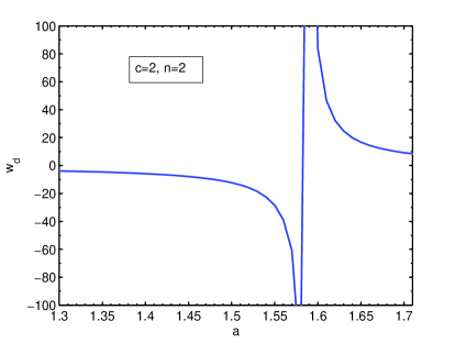
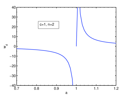
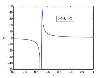
Figure 2: The singularity of polytropic gas model for different values of model parameter $c$.

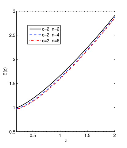
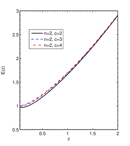
Figure 3: The evolution of dimensionless Hubble parameter as a function of redshift parameter $z$ for different values of $n$ and $c$ as described in legend.

III Tachyon reconstruction of polytropic gas model

Here we establish a correspondence between the polytropic gas model with the tachyon scalar field. We reconstruct the potential and the dynamics of tachyon field according to the evolution of polytropic gas model.
The tachyon scalar field can be considered as a source of dark energy c24 . The tachyon is an unstable field which can be used in string theory through its role in the Dirac-Born-Infeld (DBI) action to describe the D-bran action c25 . The effective Lagrangian for the tachyon field is given by

$$\mathcal{L}=-V(\phi)\sqrt{1-g^{\mu\nu}\partial_{\mu}\phi\partial_{\nu}\phi},$$

where $V(\phi)$ is the potential of tachyon field. The energy density and pressure of tachyon field are given by c25

$$\rho_{\phi}=\frac{V(\phi)}{\sqrt{1-\dot{\phi}^{2}}},$$ (13)

$$p_{\phi}=-V(\phi)\sqrt{1-\dot{\phi}^{2}}.$$ (14)

The EoS parameter of tachyon field can be given by

$$w_{\phi}=\frac{p_{\phi}}{\rho_{\phi}}=\dot{\phi}^{2}-1.$$ (15)

From (13), we see that in the case of $-1<\dot{\phi}<1$ or in the case of $\dot{\phi}^{2}<0$ tachyon field has a real energy density. Consequently, from (15), it is clear to see that in the first case the EoS parameter of tachyon is constrained to $-1<w_{\phi}<0$ and therefor the tachyon field can interpret the accelerates expansion of universe, but can not enter the phantom regime, i.e. $w_{d}<-1$. In the later case, $\dot{\phi}^{2}<0$, we see $w_{\phi}<-1$, and the phantom regime can be crossed by tachyon.
By equating the relations (9) and (15) and also (7) with (13), we reconstruct the potential and the dynamics of tachyon according to evolution of interacting polytropic gas model as follows

$$w_{d}=-1-\frac{a^{\frac{3}{n}}}{c-a^{\frac{3}{n}}}=\dot{\phi}^{2}-1.$$ (16)

$$\rho_{d}=\left(\frac{1}{Ba^{\frac{3}{n}}-K}\right)^{n}=\frac{V(\phi)}{\sqrt{1-\dot{\phi}^{2}}}$$ (17)

Therefor we obtain the following expressions for the dynamics and potential of tachyon field

$$\dot{\phi}^{2}=-\frac{a^{\frac{3}{n}}}{c-a^{\frac{3}{n}}}$$ (18)

$$V(\phi)=\sqrt{1+\frac{a^{\frac{3}{n}}}{c-a^{\frac{3}{n}}}}\left(\frac{1}{Ba^{\frac{3}{n}}-K}\right)^{n}$$ (19)

For $c>a^{3/n}$, from (18), we obtain $\dot{\phi}^{2}<0$ which represents the phantom behavior of tachyon field. By definition $\phi=i\psi$ and changing the time derivative to the derivative with respect to logarithmic scale factor, i.e. $d/dt=Hd/dx$, the scalar field $\psi$ can be integrated from (18) as follows

$$\psi(a)-\psi(a_{0})=\int_{0}^{a}{\frac{1}{aH(a)}\sqrt{\frac{a^{\frac{3}{n}}}{c-a^{\frac{3}{n}}}}}da$$ (20)

where $x=\ln{a}$ and $H(a)$ is given by (12). Here we assume the present value of scale factor as $a_{0}=1$.
The potential and the dynamics of reconstructed tachyon field according to the evolution of polytropic dark energy are given by relations (19) and (20), respectively. Unfortunately, due to the complexity of the equations involved, the above relations cannot be integrated analytically. Hence we should use the numerical method to calculate the above integrations. In figure (4), we show the evolution of the scalar field for different values of the model parameters $n$ and $c$ as a function of redshift parameter $z=1/a-1$. Here, for simplicity, we choose $\psi(z=0)=0$. We can explicitly see the dynamics of the scalar field where the scalar field decreases from up to zero at the present time. In left panel we find a faster rate of evolution when $n$ increases. Also from the right panel we see the faster evolution of dynamics of reconstructed tachyon field for lower values of model parameter $c$. In figure (5), the reconstructed tachyon potential $V(\phi)$ is plotted for different values of model parameter $n$ and $c$. Here we see that the reconstructed potential $V(\psi)$ has a nonzero minima at the early stage of universe ($z\geq 5$) which indicate the cosmological constant behavior of the model in the past time.From the left and right panels, we see the faster evolution of potential for larger values of $n$ and smaller values of $c$, respectively.

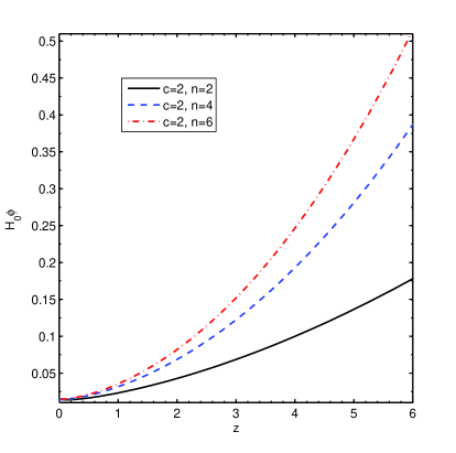
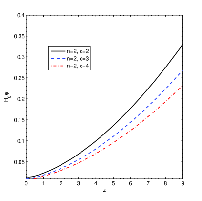
Figure 4: The evolution of scalar field $\psi$ in terms of cosmological redshift parameter $z$ for different values of $n$ and $c$ as described in legend.

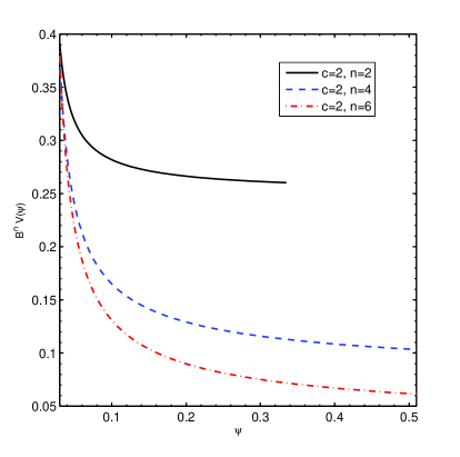
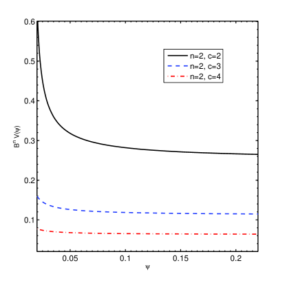
Figure 5: The reconstructed potential $V(\psi)$ for different values of model parameters of tachyon polytropic gas dark energy model as described in legend.

IV K-essence reconstruction of polytropic gas model

The propose of the K-essence scalar field was motivated from the Born-Infeld action of string theory. This kind of scalar field can interpret the late time acceleration of the universe c26 . The K-essence scalar field is given by following action c27 :

$$S=\int d^{4}x\sqrt{-g}\text{ }p(\phi,\chi),$$ (21)

where the Lagrangian density $p(\phi,\chi)$ corresponds to the pressure density and energy density via the following equations:

$$p(\phi,\chi)=f(\phi)(-\chi+\chi^{2}),$$ (22)

$$\rho(\phi,\chi)=f(\phi)(-\chi+3\chi^{2}).$$ (23)

Therefore, the EoS parameter of K-essence can be obtained as follows

$$\omega_{K}=\frac{p(\phi,\chi)}{\rho(\phi,\chi)}=\frac{\chi-1}{3\chi-1}.$$ (24)

By equating(9) and (24), we have

$$w_{d}=-1-\frac{a^{\frac{3}{n}}}{c-a^{\frac{3}{n}}}=\frac{\chi-1}{3\chi-1}$$ (25)

Therefore the parameter $\chi$ can be obtained as

$$\chi=\frac{2+\frac{a^{\frac{3}{n}}}{c-a^{\frac{3}{n}}}}{4+3\frac{a^{\frac{3}{n}}}{c-a^{\frac{3}{n}}}}$$ (26)

From (24), the phantom behavior of K-essence scalar field ($w_{K}<-1$) can be achieved when the parameter $\chi$ lies in the interval $1/3<\chi<1/2$. Using $\dot{\phi}^{2}=2\chi$ and changing the time derivative to the derivative with respect to $x=\ln{a}$, we have

$$\phi^{\prime}=\frac{1}{H}\sqrt{\frac{4+2\frac{a^{\frac{3}{n}}}{c-a^{\frac{3}{n}}}}{4+3\frac{a^{\frac{3}{n}}}{c-a^{\frac{3}{n}}}}}$$ (27)

The integration of (27) yields

$$\phi(a)-\phi(a_{0})=\int^{a}_{0}\frac{1}{aH(a)}\sqrt{\frac{4+2\frac{a^{\frac{3}{n}}}{c-a^{\frac{3}{n}}}}{4+3\frac{a^{\frac{3}{n}}}{c-a^{\frac{3}{n}}}}}da$$ (28)

The dynamics of reconstructed K-essence field via the evolutionary form of polytropic dark energy is given by (28). The K-essence polytropic gas model can explain the accelerating universe and also behaves as a phantom model provided $1/3<\chi<1/2$. Same as previous section we use the numerical method to calculate the reconstructed dynamics. In figure (6) the evolution of reconstructed K-essence is plotted as a function of cosmological redshift $z=1/a-1$ for different values of the model parameters $n$ and $c$. Here we choose $\phi(z=0)=0$. The scalar field decreases from up to zero at the present time. In left panel we find a faster rate of evolution when $n$ decreases. In right panel we see the faster evolution of dynamics of reconstructed K-essence field for higher values of model parameter $c$.

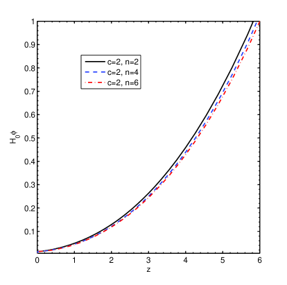
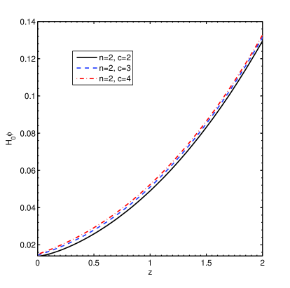
Figure 6: The evolution of scalar field $\phi$ in terms of cosmological redshift parameter $z$ for different values of $n$ and $c$ as described in legend.

V Conclusion

In summary, we considered the FRW cosmology with polytropic gas model of dark energy. The polytropic gas model can explain the cosmic acceleration of the universe and also behaves as a phantom or quintessence dark energy models, depending on the model parameters. One of the benefits of polytropic gas model is that it can cross the phantom line without a need to interaction between dark energy and dark matter. However, this model same as other phenomenological models of dark energy, suffers from the singularity. This singularity tacks place at $a_{s}=c^{n/3}$.
We also suggested a polytropic gas model of tachyon and K-essence scalar field models. We adopt the viewpoint of that the scalar field models of dark energy are effective theories of an underlying theory of dark energy. We established a connection between the scalar field models including tachyon and K-essence energy densities and the polytropic gas dark energy model. We reconstructed the potential and the dynamics of these scalar fields, numerically, according to the evolutionary form of polytropic gas dark energy model. The reconstructed scalar fields increases with redshift $z$ but. In an other words, they decreases as the universe expands. This behavior of reconstructed scalar fields via the evolution of polytropic gas model is similar with other forms of dark energy models such as tachyon reconstructed of new agegraphic model tach-age , tachyon, dilaton and quintessence reconstructed of holographic dark energy model tach-hol .

References

- (1) S. Perlmutter et al., Astrophys. J. 517, 565 (1999).
- (2) C. L. Bennett et al., Astrophys. J. Suppl. 148, 1 (2003).
- (3) M. Tegmark et al., Phys. Rev. D 69, 103501 (2004).
- (4) S. W. Allen, et al., Mon. Not. Roy. Astron. Soc. 353, 457 (2004).
- (5) S. Weinberg, Rev. Mod. Phys. 61, 1 (1989);arXiv:astro-ph/0005265; V. Sahni and A.A. Starobinsky, Int. J. Mod. Phys. D 9, 373 (2000); S.M. Carroll, Living Rev.Rel. 4, 1 (2001); P.J.E. Peebles and B. Ratra, Rev. Mod. Phys. 75, 559 (2003); T. Padmanabhan, Phys. Rept. 380, 235 (2003); E. J. Copeland, M. Sami and S. Tsujikawa, Int. J. Mod. Phys. D 15, 1753 (2006).
- (6) U. Alam, V. Sahni and A. A. Starobinsky, JCAP 0406 (2004) 008; D. Huterer and A. Cooray, Phys. Rev. D 71 (2005) 023506; Y.G. Gong, Int. J. Mod. Phys. D 14 (2005) 599; Y.G. Gong, Class. Quantum Grav. 22 (2005) 2121; Yun Wang and M. Tegmark, Phys. Rev. D 71 (2005) 103513; Yun-gui Gong and Yuan-Zhong Zhang, Phys. Rev. D 72 (2005) 043518.
-
(7)
C. Wetterich, Nucl. Phys. B 302, 668 (1988);
B. Ratra, J. Peebles, Phys. Rev. D 37, 321 (1988). -
(8)
R. R. Caldwell, Phys. Lett. B 545, 23 (2002);
S. Nojiri, S.D. Odintsov, Phys. Lett. B 562, 147 (2003);
S. Nojiri, S.D. Odintsov, Phys. Lett. B 565, 1 (2003). -
(9)
E. Elizalde, S. Nojiri, S.D. Odinstov, Phys. Rev. D 70, 043539 (2004);
S. Nojiri, S.D. Odintsov, S. Tsujikawa, Phys. Rev. D 71, 063004 (2005);
A. Anisimov, E. Babichev, A. Vikman, J. Cosmol. Astropart. Phys. 06, 006 (2005). -
(10)
T. Chiba, T. Okabe, M. Yamaguchi, Phys. Rev. D 62,
023511(2000);
C. Armend ariz-Pic on, V. Mukhanov, P.J. Steinhardt, Phys. Rev. Lett. 85, 4438 (2000);
C. Armend ariz-Pic on, V. Mukhanov, P.J. Steinhardt, Phys. Rev. D 63, 103510 (2001). -
(11)
A. Sen, J. High Energy Phys. 04, 048 (2002);
T. Padmanabhan, Phys. Rev. D 66, 021301 (2002);
T. Padmanabhan, T.R. Choudhury, Phys. Rev. D 66, 081301 (2002). - (12) M. Gasperini, F. Piazza, G. Veneziano, Phys. Rev. D 65, 023508 (2002); N. Arkani-Hamed, P. Creminelli, S. Mukohyama, M. Zaldarriaga, J. Cosmol. Astropart. Phys. 04, 001 (2004); F. Piazza, S. Tsujikawa, J. Cosmol. Astropart. Phys. 07, 004 (2004).
- (13) A. Kamenshchik, U. Moschella, V. Pasquier, Phys. Lett. B 511, 265 (2001); M. C. Bento, O. Bertolami, A. A. Sen, Phys. Rev. D 66, 043507 (2002);
- (14) M. R. Setare, Eur. Phys. J. C 52, 689, 2007.
- (15) C. Deffayet, G. R. Dvali, G. Gabadaaze, Phys. Rev. D 65, 044023 (2002); V. Sahni, Y. Shtanov, J. Cosmol. Astropart. Phys. 0311, 014 (2003).
- (16) P. Horava, D. Minic, Phys. Rev. Lett. 85, 1610 (2000); P. Horava, D. Minic, Phys. Rev. Lett. 509, 138 (2001); S. Thomas, Phys. Rev. Lett. 89, 081301 (2002); M. R. Setare, Phys. Lett. B 644, 99, 2007; M. R. Setare, Phys. Lett. B 654, 1, 2007; M. R. Setare, Phys. Lett. B 642, 1, 2006; M. R. Setare, Eur. Phys. J. C 50, 991, 2007; M. R. Setare, Phys. Lett. B 648, 329, 2007; M. R. Setare, Phys. Lett. B 653, 116, 2007.
- (17) R.G. Cai, Phys. Lett. B 657, (2007) 228; H. Wei, R.G. Cai, Phys. Lett. B 660, 113 (2008).
- (18) G. t Hooft, gr-qc/9310026; L. Susskind, J. Math. Phys. 36, 6377 (1995).
- (19) F. Karolyhazy, Nuovo.Cim. A 42 (1966) 390; F. Karolyhazy, A. Frenkel and B. Lukacs, in Physics as natural Philosophy edited by A. Shimony and H. Feschbach, MIT Press, Cambridge, MA, (1982); F. Karolyhazy, A. Frenkel and B. Lukacs, in Quantum Concepts in Space and Time edited by R. Penrose and C.J. Isham, Clarendon Press, Oxford, (1986).
- (20) J. Christensen-Dalsgard, Lecture Notes on Stellar Structure and Evolution, 6th edn. (Aarhus University Press, Aarhus, 2004).
- (21) U. Mukhopadhyay and S. Ray, Mod. Phys. Lett. A 23, 3198,2008.
- (22) K. Karami, A. Abdolmaleki, Astrophys. Space Sci.330, 133,2010.
- (23) K. Karami, S. Ghaffari, J. Fehri, Eur. Phys. J. C, 64, 85 (2009).
- (24) K. Karami, A. Abdolmaleki, arXiv:1009.3587.
- (25) M. Malekjani, A. Khodam-Mohammadi, M. Taji, Int. J. Theor. Phys. 50, 312, 2011.
- (26) M. Malekjani, A. Khodam-Mohammadi, Int. J. Theor. Phys. DOI: (2012).
- (27) X. Zhang, Phys. Lett. B 648, 1 (2007) [arXiv:astro-ph/0604484]; X. Zhang, Phys. Rev. D 74, 103505 (2006) [arXiv:astro-ph/0609699]; J. Zhang, X. Zhang and H. Liu, Phys. Lett. B 651, 84 (2007) [arXiv:0706.1185 [astro-ph]]; Y. Z. Ma and X. Zhang, Phys. Lett. B 661, 239 (2008) [arXiv:0709.1517 [astro-ph]]; N. Cruz, P. F. Gonzalez-Diaz, A. Rozas-Fernandez and G. Sanchez, arXiv:0812.4856 [grqc]; I. P. Neupane, Phys. Rev. D 76, 123006 (2007) [arXiv:0709.3096 [hep-th]]; J. Zhang, X. Zhang and H. Liu, Eur. Phys. J. C 54, 303 (2008) [arXiv:0801.2809 [astro-ph]]; J. P. Wu, D. Z. Ma and Y. Ling, Phys. Lett. B 663, 152 (2008) [arXiv:0805.0546 [hep-th]]; X. Zhang, arXiv:0901.2262 [astroph.CO]; C. J. Feng, arXiv:0810.2594 [hep-th]; X. Wu and Z. H. Zhu, Phys. Lett. B 660, 293 (2008) [arXiv:0712.3603 [astro-ph]]; M. R. Setare, Phys. Lett. B 648, 329 (2007) [arXiv:0704.3679 [hep-th]].
- (28) S. Nojiri, S. D. Odintsov, S. Tsujikawa, Phys. Rev. D 71, 063004 (2005).
- (29) J. S. Bagla, H. K. Jassal, T. Padmanabhan, Phys. Rev. D 67, 063504 (2003), astro-ph/0212198 Ying Shao, Yuan-Xing Gui and Wei Wang, Mod. Phys. Lett. A 22, 1175-1182 (2007), gr-qc/0703112 Gianluca Calcagni and Andrew R. Liddle, Phys. Rev. D 74, 043528,2006, astro-ph/0606003 Edmund J. Copeland, Mohammad R. Garousi, M. Sami and Shinji Tsujikawa, Phys. Rev. D 71, 043003 (2005), hep-th/0411192
- (30) A. Sen, JHEP 0204, 048 (2002); JHEP 0207, 065 (2002); Mod. Phys. Lett. A 17, 1797 (2002); arXiv: hep- th/0312153;A. Sen, JHEP 9910, 008 (1999); E. A. Bergshoeff, M. de Roo, T. C. de Wit, E. Eyras, S. Panda, JHEP 0005, 009 (2000); J. Kluson, Phys. Rev. D 62, 126003 (2000); D. Kutasov and V. Niarchos, Nucl. Phys. B 666, 56, (2003).
- (31) D. N. Spergel, et al., Satrophys. J. Suppl. 170, 377 (2007).
- (32) J. Christensen-Dalsgard, Lecture Notes on Stellar Structure and Evolution, 6th edn. (Aarhus University Press, Aarhus, 2004).
- (33) K. Karami, S. Ghaffari, J. Fehri, Eur. Phys. J. C, 64, 85 (2009).
- (34) S. Nojiri, S. D. Odintsov, S. Tsujikawa, Phys. Rev. D 71, 063004 (2005).
-
(35)
H. Wei, R. G. Cai, Eur.Phys.J.C 59, 99, 2009;
H. Wei, R. G. Cai, Phys. Lett. B 660, 113, 2008. - (36) M. R. Setare, Phys. Lett. B 642, 1, 2006.
- (37) A. Sen, Mod. Phys. Lett. A 17 (2002) 1797; N. D. Lambert, I. Sachs, Phys. Rev. D 67 (2003) 026005.
- (38) T. Chiba et al., Phys. Rev. D 62 (2000) 023511; C. Armendariz-Picon et al., Phys. Rev. Lett 85 (2000) 4438; C. Armendariz-Picon et al., Phys. Rev. Lett 63 (2001) 103510.
- (39) F. Piazza and S. Tsujikawa, JCAP 0407, 004 (2004).
- (40) J. Cui, L. Zhang, J. Zhang, and X. Zhang, Chin. Phys. B 19, 019802-6, 2010.
-
(41)
A. Rozas-Fernandez, D. Brizuela, N. Cruz, Int. J. Mod. Phys. D 19,
573 (2010);
A. Rozas-Fernandez, Eur. Phys. J. C 71:1536,2011;
X. Zhang, Phys. Lett. B 648:1-7, 2007 ;
J. Zhang, X. Zhang and H. Liu, Phys. Lett. B 651, 84-88, 2007.