Factor modeling for high-dimensional time series: Inference for the number of factors

Abstract

This paper deals with the factor modeling for high-dimensional time series based on a dimension-reduction viewpoint. Under stationary settings, the inference is simple in the sense that both the number of factors and the factor loadings are estimated in terms of an eigenanalysis for a nonnegative definite matrix, and is therefore applicable when the dimension of time series is on the order of a few thousands. Asymptotic properties of the proposed method are investigated under two settings: (i) the sample size goes to infinity while the dimension of time series is fixed; and (ii) both the sample size and the dimension of time series go to infinity together. In particular, our estimators for zero-eigenvalues enjoy faster convergence (or slower divergence) rates, hence making the estimation for the number of factors easier. In particular, when the sample size and the dimension of time series go to infinity together, the estimators for the eigenvalues are no longer consistent. However, our estimator for the number of the factors, which is based on the ratios of the estimated eigenvalues, still works fine. Furthermore, this estimation shows the so-called “blessing of dimensionality” property in the sense that the performance of the estimation may improve when the dimension of time series increases. A two-step procedure is investigated when the factors are of different degrees of strength. Numerical illustration with both simulated and real data is also reported.

abstractwidth290pt

T1Supported in part by the Engineering and Physical Sciences Research Council of the United Kingdom.

and

1 Introduction

The analysis of multivariate time series data is of increased interest and importance in the modern information age. Although the methods and the associate theory for univariate time series analysis are well developed and understood, the picture for the multivariate cases is less complete. In spite of the fact that the conventional univariate time series models (such as ARMA) and the associated time-domain and frequency-domain methods have been formally extended to multivariate cases, their usefulness is often limited. One may face serious issues such as the lack of model identification or flat likelihood functions. In fact vector ARMA models are seldom used directly in practice. Dimension-reduction via, for example, reduced-rank structure, structural indices, scalar component models and canonical correlation analysis is more pertinent in modeling multivariate time series data. See H70 , P81 , L93 , R97 .

In this paper we deal with the factor modeling for multivariate time series from a dimension-reduction viewpoint. Differently from the factor analysis for independent observations, we search for the factors which drive the serial dependence of the original time series. Early attempts in this direction include A63 , PRT74 , B81 , SG84 , PB87 , SS89 , PY08 . More recent efforts focus on the inference when the dimension of time series is as large as or even greater than the sample size; see, for example, LYB11 and the references within. High-dimensional time series data are often encountered nowadays in many fields including finance, economics, environmental and medical studies. For example, understanding the dynamics of the returns of large numbers of assets is the key for asset pricing, portfolio allocation, and risk management. Panel time series are commonplace in studying economic and business phenomena. Environmental time series are often of a high dimension due to a large number of indices monitored across many different locations.

Our approach is from a dimension-reduction point of view. The model adopted can be traced back at least to that of PB87 . We decompose a high-dimensional time series into two parts: a dynamic part driven by, hopefully, a lower-dimensional factor time series, and a static part which is a vector white noise. Since the white noise exhibits no serial correlations, the decomposition is unique in the sense that both the number of factors (i.e., the dimension of the factor process) and the factor loading space in our model are identifiable. Such a conceptually simple decomposition also makes the statistical inference easy. Although the setting allows the factor process to be nonstationary (see PY08 ; also Section 2.1 below), we focus on stationary models only in this paper: under the stationary condition, the estimation for both the number of factors and the factor loadings is carried out in an eigenanalysis for a nonnegative definite matrix, and is therefore applicable when the dimension of time series is on the order of a few thousands. Furthermore, the asymptotic properties of the proposed method are investigated under two settings: (i) the sample size goes to infinity while the dimension of time series is fixed; and (ii) both the sample size and the dimension of time series go to infinity together. In particular, our estimators for zero-eigenvalues enjoy the faster convergence (or slower divergence) rates, from which the proposed ratio-based estimator for the number of factors benefits. In fact when all the factors are strong, the performance of our estimation for the number of factors improves when the dimension of time series increases. This phenomenon is coined as “blessing of dimensionality.”

The new contributions of this paper include: (i) the ratio-based estimator for the number of factors and the associated asymptotic theory which underpins the “blessing of dimensionality” phenomenon observed in numerical experiments, and (ii) a two-step estimation procedure when the factors are of different degrees of strength. We focus on the results related to the estimation for the number of factors in this paper. The results on the estimation of the factor loading space under the assumption that the number of factors is known are reported in LYB11 .

There exists a large body of literature in econometrics and finance on factor models for high-dimensional time series. However, most of them are based on a different viewpoint, as those models attempt to identify the common factors that affect the dynamics of most original component series. In analyzing economic and financial phenomena, it is often appealing to separate these common factors from the so-called idiosyncratic components: each idiosyncratic component may at most affect the dynamics of a few original time series. An idiosyncratic series may exhibit serial correlations and, therefore, may be a time series itself. This poses technical difficulties in both model identification and inference. In fact the rigorous definition of the common factors and the idiosyncratic components can only be established asymptotically when the dimension of time series tends to infinity; see CR83 , FHLR00 . Hence those factor models are only asymptotically identifiable. According to the definition adopted in this paper, both “the common factors” and those serially correlated idiosyncratic components will be identified as factors. This is not ideal for the applications with the purpose to identify those common factors. However, this makes the tasks of model identification and inference much simpler.

The rest of the paper is organized as follows. The model and the estimation methods are introduced in Section 2. The sampling properties of the estimation methods are investigated in Section 3. Simulation results are inserted whenever appropriate to illustrate the various asymptotic properties of the methods. Section 4 deals with the cases when different factors are of different strength, for which a two-step estimation procedure is preferred. The analysis of two real data sets is reported in Section 5. All mathematical proofs are relegated to the Appendix.

2 Models and estimation

2.1 Models

If we are interested in the linear dynamic structure of ${\mathbf{y}}_{t}$ only, conceptually we may think that ${\mathbf{y}}_{t}$ consists of two parts: a static part (i.e., a white noise), and a dynamic component driven by, hopefully, a low-dimensional process. This leads to the decomposition:

$${\mathbf{y}}_{t}={\mathbf{A}}{\mathbf{x}}_{t}+\bolds\varepsilon_{t},$$ (1)

where ${\mathbf{x}}_{t}$ is an $r\times 1$ latent process with (unknown) $r\leq p$, ${\mathbf{A}}$ is a $p\times r$ unknown constant matrix, and $\bolds\varepsilon_{t}\sim\mathrm{WN}(\bolds{\mu}_{\varepsilon},\bolds{\Sigma}_{\varepsilon})$ is a vector white-noise process. When $r$ is much smaller than $p$, we achieve an effective dimension-reduction, as then the serial dependence of ${\mathbf{y}}_{t}$ is driven by that of a much lower-dimensional process ${\mathbf{x}}_{t}$. We call ${\mathbf{x}}_{t}$ a factor process. The setting (1) may be traced back at least to PB87 ; see also its further development in dealing with cointegrated factors in PP06 .

Since none of the elements on the RHS of (1) are observable, we have to characterize them further to make them identifiable. First we assume that no linear combinations of ${\mathbf{x}}_{t}$ are white noise, as any such components can be absorbed into $\bolds\varepsilon_{t}$ [see condition (C1) below]. We also assume that the rank of ${\mathbf{A}}$ is $r$. Otherwise (1) may be expressed equivalently in terms of a lower-dimensional factor. Furthermore, since (1) is unchanged if we replace $({\mathbf{A}},{\mathbf{x}}_{t})$ by $({\mathbf{A}}{\mathbf{H}},{\mathbf{H}}^{-1}{\mathbf{x}}_{t})$ for any invertible $r\times r$ matrix ${\mathbf{H}}$, we may assume that the columns of ${\mathbf{A}}=({\mathbf{a}}_{1},\ldots,{\mathbf{a}}_{r})$ are orthonormal, that is, ${\mathbf{A}}^{\prime}{\mathbf{A}}={\mathbf{I}}_{r}$, where ${\mathbf{I}}_{r}$ denotes the $r\times r$ identity matrix. Note that even with this constraint, ${\mathbf{A}}$ and ${\mathbf{x}}_{t}$ are not uniquely determined in (1), as the aforementioned replacement is still applicable for any orthogonal ${\mathbf{H}}$. However, the factor loading space, that is, the $r$-dimensional linear space spanned by the columns of ${\mathbf{A}}$, denoted by ${\mathcal{M}}({\mathbf{A}})$, is uniquely defined.

We summarize into condition (C1) all the assumptions introduced so far: [(C1)]

In model (1), $\bolds\varepsilon_{t}\sim\mathrm{WN}(\bolds{\mu}_{{\varepsilon}},\bolds{\Sigma}_{{\varepsilon}})$. If ${\mathbf{c}}^{\prime}{\mathbf{X}}_{t}$ is white noise for a constant ${\mathbf{c}}\in\mathcal{R}^{p}$, then ${\mathbf{c}}^{\prime}\operatorname{Cov}({\mathbf{X}}_{t+k},\bolds\varepsilon_{t})=\mathbf{0}$ for any nonzero integers $k$. Furthermore ${\mathbf{A}}^{\prime}{\mathbf{A}}={\mathbf{I}}_{r}$.

The key for the inference for model (1) is to determine the number of factors $r$ and to estimate the $p\times r$ factor loading matrix ${\mathbf{A}}$, or more precisely the factor loading space ${\mathcal{M}}({\mathbf{A}})$. Once we have obtained an estimator, say, $\widehat{\mathbf{A}}$, a natural estimator for the factor process is

$$\widehat{\mathbf{x}}_{t}=\widehat{\mathbf{A}}^{\prime}{\mathbf{y}}_{t},$$ (2)

and the resulting residuals are

$$\widehat{\bolds}\varepsilon_{t}=({\mathbf{I}}_{d}-\widehat{\mathbf{A}}\widehat{\mathbf{A}}^{\prime}){\mathbf{y}}_{t}.$$ (3)

The dynamic modeling for ${\mathbf{y}}_{t}$ is achieved via such a modeling for $\widehat{\mathbf{x}}_{t}$ and the relationship $\widehat{\mathbf{y}}_{t}=\widehat{\mathbf{A}}\widehat{\mathbf{x}}_{t}$. A parsimonious fitting for $\widehat{\mathbf{x}}_{t}$ may be obtained by rotating $\widehat{\mathbf{x}}_{t}$ appropriately TT89 . Such a rotation is equivalent to replacing $\widehat{\mathbf{A}}$ by $\widehat{\mathbf{A}}{\mathbf{H}}$ for an appropriate $r\times r$ orthogonal matrix ${\mathbf{H}}$. Note that ${\mathcal{M}}(\widehat{\mathbf{A}})={\mathcal{M}}(\widehat{\mathbf{A}}{\mathbf{H}})$, and the residuals (3) are unchanged with such a replacement.

2.2 Estimation for ${\mathbf{A}}$ and $r$

An innovation expansion algorithm is proposed in PY08 for estimating ${\mathbf{A}}$ based on solving a sequence of nonlinear optimization problems with at most $p$ variables. Although the algorithm is feasible for small or moderate $p$ only, it can handle the situations when the factor process ${\mathbf{x}}_{t}$ is nonstationary. We outline the key idea below, as our computationally more efficient estimation method for stationary cases is based on the same principle.

Our goal is to estimate ${\mathcal{M}}({\mathbf{A}})$, or, equivalently, its orthogonal complement ${\mathcal{M}}({\mathbf{B}})$, where ${\mathbf{B}}=({\mathbf{b}}_{1},\ldots,{\mathbf{b}}_{p-r})$ is a $p\times(p-r)$ matrix for which $({\mathbf{A}},{\mathbf{B}})$ forms a $p\times p$ orthogonal matrix, that is, ${\mathbf{B}}^{\prime}{\mathbf{A}}=0$ and ${\mathbf{B}}^{\prime}{\mathbf{B}}={\mathbf{I}}_{p-r}$ [see also (C1)]. It follows from (1) that

$${\mathbf{B}}^{\prime}{\mathbf{y}}_{t}={\mathbf{B}}^{\prime}\bolds\varepsilon_{t},$$ (4)

implying that for any $1\leq j\leq p-r$, $\{{\mathbf{b}}_{j}^{\prime}{\mathbf{y}}_{t},t=0,\pm 1,\ldots\}$ is a white-noise process. Hence, we may search for mutually orthogonal directions ${\mathbf{b}}_{1},{\mathbf{b}}_{2},\ldots$ one by one such that the projection of ${\mathbf{y}}_{t}$ on each of those directions is a white noise. We stop the search when such a direction is no longer available, and take $p-k$ as the estimated value of $r$, where $k$ is the number of directions obtained in the search. This is essentially how PY08 accomplish the estimation. It is irrelevant in the above derivation if ${\mathbf{x}}_{t}$ is stationary or not.

However, a much simpler method is available when ${\mathbf{x}}_{t}$, therefore also ${\mathbf{y}}_{t}$, is stationary: [(C2)]

${\mathbf{x}}_{t}$ is weakly stationary, and Cov$({\mathbf{x}}_{t},\bolds\varepsilon_{t+k})=0$ for any $k\geq 0$. In most factor modeling literature, ${\mathbf{x}}_{t}$ and $\bolds\varepsilon_{s}$ are assumed to be uncorrelated for any $t$ and $s$. Condition (C2) requires only that the future white-noise components are uncorrelated with the factors up to the present. This enlarges the model capacity substantially. Put

$$\bolds{\Sigma}_{y}(k) = \operatorname{Cov}({\mathbf{y}}_{t+k},{\mathbf{y}}_{t}),\qquad\bolds{\Sigma}_{x}(k)=\operatorname{Cov}({\mathbf{x}}_{t+k},{\mathbf{x}}_{t}),$$

$$\bolds{\Sigma}_{x{\varepsilon}}(k) = \operatorname{Cov}({\mathbf{x}}_{t+k},\bolds\varepsilon_{t}).$$

It follows from (1) and (C2) that

$$\bolds{\Sigma}_{y}(k)={\mathbf{A}}\bolds{\Sigma}_{x}(k){\mathbf{A}}^{\prime}+{\mathbf{A}}\bolds{\Sigma}_{x{\varepsilon}}(k),\qquad k\geq 1.$$ (5)

For a prescribed integer $k_{0}\geq 1$, define

$${\mathbf{M}}=\sum_{k=1}^{k_{0}}\bolds{\Sigma}_{y}(k)\bolds{\Sigma}_{y}(k)^{\prime}.$$ (6)

Then ${\mathbf{M}}$ is a $p\times p$ nonnegative matrix. It follows from (5) that ${\mathbf{M}}{\mathbf{B}}=0$, that is, the columns of ${\mathbf{B}}$ are the eigenvectors of ${\mathbf{M}}$ corresponding to zero-eigenvalues. Hence conditions (C1) and (C2) imply:

The factor loading space ${\mathcal{M}}({\mathbf{A}})$ is spanned by the eigenvectors of ${\mathbf{M}}$ corresponding to its nonzero eigenvalues, and the number of the nonzero eigenvalues is $r$.

We take the sum in the definition of ${\mathbf{M}}$ to accumulate the information from different time lags. This is useful especially when the sample size $n$ is small. We use the nonnegative definite matrix $\bolds{\Sigma}_{y}(k)\bolds{\Sigma}_{y}(k)^{\prime}$ [instead of $\bolds{\Sigma}_{y}(k)$] to avoid the cancellation of the information from different lags. This is guaranteed by the fact that for any matrix ${\mathbf{C}}$, ${\mathbf{M}}{\mathbf{C}}=0$ if and only if $\bolds{\Sigma}_{y}(k)^{\prime}{\mathbf{C}}=0$ for all $1\leq k\leq k_{0}$. We tend to use small $k_{0}$, as the autocorrelation is often at its strongest at the small time lags. On the other hand, adding more terms will not alter the value of $r$, although the estimation for $\bolds{\Sigma}_{y}(k)$ with large $k$ is less accurate. The simulation results reported in LYB11 also confirm that the estimation for ${\mathbf{A}}$ and $r$, defined below, is not sensitive to the choice of $k_{0}$.

To estimate ${\mathcal{M}}({\mathbf{A}})$, we only need to perform an eigenanalysis on

$$\widehat{\mathbf{M}}=\sum_{k=1}^{k_{0}}\widehat{\bolds}{\Sigma}_{y}(k)\widehat{\bolds}{\Sigma}_{y}(k)^{\prime},$$ (7)

where $\widehat{\bolds}{\Sigma}_{y}(k)$ denotes the sample covariance matrix of ${\mathbf{y}}_{t}$ at lag $k$. Then the estimator $\widehat{r}$ for the number of factors is defined in (8) below. The columns of the estimated factor loading matrix $\widehat{\mathbf{A}}$ are the $\widehat{r}$ orthonormal eigenvectors of $\widehat{\mathbf{M}}$ corresponding to its $\widehat{r}$ largest eigenvalues. Note that the estimator $\widehat{\mathbf{A}}$ is essentially the same as that defined in Section 2.4 of LYB11 , although a canonical form of the model is used there in order to define the factor loading matrix uniquely.

Due to the random fluctuation in a finite sample, the estimates for the zero-eigenvalues of ${\mathbf{M}}$ are unlikely to be 0 exactly. A common practice is to plot all the estimated eigenvalues in a descending order, and look for a cut-off value $\widehat{r}$ such that the $(\widehat{r}+1)$th largest eigenvalue is substantially smaller than the $\widehat{r}$ largest eigenvalues. This is effectively an eyeball-test. The ratio-based estimator defined below may be viewed as an enhanced eyeball-test, based on the same idea as W10 . In fact this ratio-based estimator benefits from the faster convergence rates of the estimators for the zero-eigenvalues; see Proposition 1 in Section 3.1 below, and also Theorems 1 and 2 in Section 3.2 below. The other available methods for determining $r$ include the information criteria approaches of BN02 , BN07 and HL07 , and the bootstrap approach of BYZ10 , though the settings considered in those papers are different.

A ratio-based estimator for $r$. We define an estimator for the number of factors $r$ as follows:

$$\widehat{r}=\mathop{\arg\min}_{1\leq i\leq R}\widehat{\lambda}_{i+1}/\widehat{\lambda}_{i},$$ (8)

where $\widehat{\lambda}_{1}\geq\cdots\geq\widehat{\lambda}_{p}$ are the eigenvalues of $\widehat{\mathbf{M}}$, and $r<R<p$ is a constant.

In practice we may use, for example, $R=p/2$. We cannot extend the search up to $p$, as the minimum eigenvalue of $\widehat{\mathbf{M}}$ is likely to be practically 0, especially when $n$ is small and $p$ is large. It is worthy noting that when $p$ and $n$ are on the same order, the estimators for eigenvalues are no longer consistent. However, the ratio-based estimator (8) still works well. See Theorem 2(iii) below.

The above estimation methods for ${\mathbf{A}}$ and $r$ can be extended to those nonstationary time series for which a generalized lag-$k$ autocovariance matrix is well defined (see, e.g., PP06 ). In fact, the methods are still applicable when the weak limit of the generalized lag-$k$ autocovariance matrix

$$\widehat{\mathbf{S}}_{y}(k)=n^{-\alpha}\sum_{t=1}^{n-1}({\mathbf{y}}_{t+k}-\bar{{\mathbf{y}}})({\mathbf{y}}_{t}-\bar{{\mathbf{y}}})^{\prime}$$

exists for $1\leq k\leq k_{0}$, where $\alpha>1$ is a constant. Further developments on those lines will be reported elsewhere. For the factor modeling for high-dimensional volatility processes based on a similar idea, we refer to PPPY11 , TWYZ11 .

3 Estimation properties

Conventional asymptotic properties are established under the setting that the sample size $n$ tends to $\infty$ and everything else remains fixed. Modern time series analysis encounters the situation when the number of time series $p$ is as large as, or even larger than, the sample size $n$. Then the asymptotic properties established under the setting when both $n$ and $p$ tend to $\infty$ are more relevant. We deal with these two settings in Section 3.1 and Sections 3.2–3.4 separately.

3.1 Asymptotics when $n\to\infty$ and $p$ fixed

We first consider the asymptotic properties under the assumption that $n\to\infty$ and $p$ is fixed. These properties reflect the behavior of our estimation method in the cases when $n$ is large and $p$ is small. We introduce some regularity conditions first. Let $\lambda_{1},\ldots,\lambda_{p}$ be the eigenvalues of the matrix ${\mathbf{M}}$: [(C3)]

${\mathbf{y}}_{t}$ is strictly stationary and $\psi$-mixing with the mixing coefficients $\psi(\cdot)$ satisfying the condition that $\sum_{t\geq 1}t\psi(t)^{1/2}<\infty$. Furthermore, $E\{|{\mathbf{y}}_{t}|^{4}\}<\infty$ element-wisely.

$\lambda_{1}>\cdots>\lambda_{r}>0=\lambda_{r+1}=\cdots=\lambda_{p}$.

Section 2.6 of FY03 gives a compact survey on the mixing properties of time series. The use of the $\psi$-mixing condition in (C3) is for technical convenience. Note that ${\mathbf{M}}$ is a nonnegative definite matrix. All its eigenvalues are nonnegative. Condition (C4) assumes that its $r$ nonzero eigenvalues are distinct from each other. While this condition is not essential, it substantially simplifies the presentation of the convergence properties in Proposition 1 below. Let $\bolds{\gamma}_{j}$ be a unit eigenvector of ${\mathbf{M}}$ corresponding to the eigenvalue $\lambda_{j}$. We denote by $(\widehat{\lambda}_{1},\widehat{\bolds}{\gamma}_{1}),\ldots,(\widehat{\lambda}_{p},\widehat{\bolds}{\gamma}_{p})$ the $p$ pairs of eigenvalue and eigenvector of matrix $\widehat{\mathbf{M}}$: the eigenvalues $\widehat{\lambda}_{j}$ are arranged in descending order, and the eigenvectors $\widehat{\bolds}{\gamma}_{j}$ are orthonormal. Furthermore, it may go without explicit statement that $\widehat{\bolds}{\gamma}_{j}$ may be replaced by $-\widehat{\bolds}{\gamma}_{j}$ in order to match the direction of $\bolds{\gamma}_{j}$ for $1\leq j\leq r$.

Proposition 1

Let conditions (C1)–(C4) hold. Then as $n\to\infty$ (but $p$ fixed), it holds that:

$|\widehat{\lambda}_{j}-\lambda_{j}|=O_{P}(n^{-1/2})$ and $\|\widehat{\bolds}{\gamma}_{j}-\bolds{\gamma}_{j}\|=O_{P}(n^{-1/2})$ for $j=1,\ldots,r$, and

$\widehat{\lambda}_{j}=O_{P}(n^{-1})$ for $j=r+1,\ldots,p$.

The proof of the above proposition is in principle the same as that of Theorem 1 in BYZ10 , and is therefore omitted.

3.2 Asymptotics when $n\to\infty,p\to\infty$ and $r$ fixed

To highlight the radically different behavior when $p$ diverges together with $n$, we first conduct some simulations: we set in model (1) $r=1$, ${\mathbf{A}}^{\prime}=(1,\ldots,1)$, $\bolds\varepsilon_{t}$ are independent $N(0,{\mathbf{I}}_{p})$, and ${\mathbf{x}}_{t}=x_{t}$ is an AR(1) process defined by $x_{t+1}=0.7x_{t}+e_{t}.$ We set the sample size $n=50,100,200,400$, $800,1600$ and 3200, and the dimension fixed at half the sample size, that is, $p=n/2$. Let ${\mathbf{M}}$ be defined as in (6) with $k_{0}=1$. For each setting, we draw 200 samples. The boxplots of the errors $\widehat{\lambda}_{i}-\lambda_{i}$, $i=1,\ldots,6$, are depicted in Figure 1. Note that $\lambda_{i}=0$ for $i\geq 2$, since $r=1$.

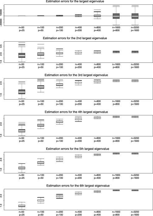
Figure 1: Boxplots for the errors in estimating the first six eigenvalues of ${\mathbf{M}}$ with $r=1$ and all the factor loading coefficients being 1.

The figure shows that those estimation errors do not converge to 0. In fact those errors seem to increase when $n$ (and also $p=n/2$) increases. Therefore the classical asymptotic theory (i.e., $n\to\infty$ and $p$ fixed) such as Proposition 1 above is irrelevant when $p$ increases together with $n$. In spite of the lack of consistency in estimating the eigenvalues, the ratio-based estimator for the number of factors $r$ ($=$1) defined in (8) works perfectly fine for this example, as shown in Figure 2. In fact it is always the case that $\widehat{r}\equiv 1$ in all our experiments even when the sample size is as small as $n=50$; see Figure 2.

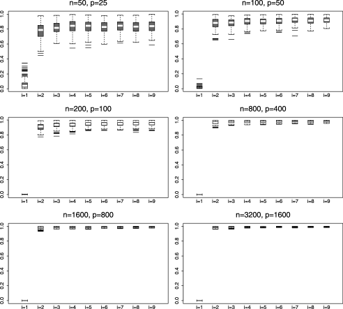
Figure 2: Boxplots for the ratios $\widehat{\lambda}_{i+1}/\widehat{\lambda}_{i}$, with $r=1$ and all the factor loading coefficients being 1.

To develop the relevant asymptotic theory, we introduce some notation first. For any matrix ${\mathbf{G}}$, let $\|{\mathbf{G}}\|$ be the square root of the maximum eigenvalue of ${\mathbf{G}}{\mathbf{G}}^{\prime}$, and $\|{\mathbf{G}}\|_{\min}$ be the square root of the smallest nonzero eigenvalue of ${\mathbf{G}}{\mathbf{G}}^{\prime}$. We write $a\asymp b$ if $a=O(b)$ and $b=O(a)$. Recall $\bolds{\Sigma}_{x}(k)=\operatorname{Cov}({\mathbf{x}}_{t+k},{\mathbf{x}}_{t})$ and $\bolds{\Sigma}_{x\epsilon}(k)=\operatorname{Cov}({\mathbf{x}}_{t+k},\bolds\varepsilon_{t})$. Some regularity conditions are now in order: [(C5)]

For a constant $\delta\in[0,1]$, it holds that $\|\bolds{\Sigma}_{x}(k)\|\asymp p^{1-\delta}\asymp\|\bolds{\Sigma}_{x}(k)\|_{\min}$.

For $k=0,1,\ldots,k_{0}$, $\|\bolds{\Sigma}_{x\epsilon}(k)\|=o(p^{1-\delta})$.

Remark 1.

(i) Condition (C5) looks unnatural. It is derived from more natural conditions (9) and (10) below coupled with the standardization ${\mathbf{A}}^{\prime}{\mathbf{A}}={\mathbf{I}}_{r}$. Since ${\mathbf{A}}=({\mathbf{a}}_{1},\ldots,{\mathbf{a}}_{r})$ is $p\times r$ and $p\to\infty$ now, it is natural to let the norm of each column of ${\mathbf{A}}$, before standardizing to ${\mathbf{A}}^{\prime}{\mathbf{A}}={\mathbf{I}}_{r}$, tend to $\infty$ as well. To this end, we assume that

$$\|{\mathbf{a}}_{j}\|^{2}\asymp p^{1-\delta_{j}},\qquad j=1,\ldots,r,$$ (9)

where $\delta_{j}\in[0,1]$ are constants. We take $\delta_{j}$ as a measure of the strength of the factor $x_{tj}$. We call $x_{tj}$ a strong factor when $\delta_{j}=0$, and a weak factor when $\delta_{j}>0$. Since $r$ is fixed, it is also reasonable to assume that for $k=0,1,\ldots,k_{0}$,

$$|\bolds{\Sigma}_{x}(k)|\neq 0.$$ (10)

Then condition (C5) is entailed by the standardization ${\mathbf{A}}^{\prime}{\mathbf{A}}={\mathbf{I}}_{r}$ under conditions (10) and (9) with $\delta_{j}=\delta$ for all $j$.

(ii) The condition assumed on $\bolds{\Sigma}_{x\epsilon}(k)$ in (C6) requires that the correlation between ${\mathbf{x}}_{t+k}$ ($k\geq 0$) and $\bolds\varepsilon_{t}$ is not too strong. In fact under a natural condition that $\bolds{\Sigma}_{x\epsilon}(k)=O(1)$ element-wisely, it is implied by (9) and the standardization ${\mathbf{A}}^{\prime}{\mathbf{A}}={\mathbf{I}}_{r}$ [hence now $x_{j,t}=O_{P}(p^{(1-\delta)/2})$ as a result of such standardization] that $\|\bolds{\Sigma}_{x\epsilon}(k)\|=O(p^{1-\delta/2})$.

Now we deal with the convergence rates of the estimated eigenvalues, and establish the results in the same spirit as Proposition 1. Of course the convergence (or divergence) rate for each estimator $\widehat{\lambda}_{i}$ is slower, as the number of estimated parameters goes to infinity now.

Theorem 1

Let conditions (C1)–(C6) hold and $h_{n}=p^{\delta}n^{-1/2}\to 0$. Then as $n\to\infty$ and $p\to\infty$, it holds that:

$|\widehat{\lambda}_{i}-\lambda_{i}|=O_{P}(p^{2-\delta}n^{-1/2})$ for $i=1,\ldots,r$, and

$\widehat{\lambda}_{j}=O_{P}(p^{2}n^{-1})$ for $j=r+1,\ldots,p$.

Corollary 1

Under the condition of Theorem 1, it holds that

$$\widehat{\lambda}_{j+1}/\widehat{\lambda}_{j}\asymp 1\qquad\mbox{for }j=1,\ldots,r-1\quad\mbox{and}\quad\widehat{\lambda}_{r+1}/\widehat{\lambda}_{r}=O_{P}(p^{2\delta}/n)\stackrel{{\scriptstyle P}}{{\longrightarrow}}0.$$

The proofs of Theorem 1 and Corollary 1 are presented in the Appendix. Obviously when $p$ is fixed, Theorem 1 formally reduces to Proposition 1. Some remarks are now in order.

Remark 2.

(i) Corollary 1 implies that the plot of ratios $\widehat{\lambda}_{i+1}/\widehat{\lambda}_{i}$, $i=1,2,\ldots,$ will drop sharply at $i=r$. This provides a partial theoretical underpinning for the estimator $\widehat{r}$ defined in (8). Especially when all factors are strong (i.e., $\delta=0$), $\widehat{\lambda}_{r+1}/\widehat{\lambda}_{r}=O_{P}(n^{-1})$. This convergence rate is independent of $p$, suggesting that the estimation for $r$ may not suffer as $p$ increases. In fact when all the factors are strong, the estimation for $r$ may improve as $p$ increases. See Remark 3(iv) in Section 3.4 below.

(ii) Unfortunately, we are unable to derive an explicit asymptotic expression for the ratios $\widehat{\lambda}_{i+1}/\widehat{\lambda}_{i}$ with $i>r$, although we make the following conjecture:

$$\widehat{\lambda}_{j+1}/\widehat{\lambda}_{j}\stackrel{{\scriptstyle P}}{{\longrightarrow}}1,\qquad j=(k_{0}+1)r+1,\ldots,(k_{0}+1)r+K,$$ (11)

where $k_{0}$ is the number of lags used in defining matrix ${\mathbf{M}}$ in (6), and $K\geq 1$ is any fixed integer. See also Figure 2. Further simulation results, not reported explicitly, also conform with (11). This conjecture arises from the following observation: for $j>(k_{0}+1)r$, the $j$th largest eigenvalue of $\widehat{\mathbf{M}}$ is predominately contributed by the term $\sum_{k=1}^{k_{0}}\widehat{\bolds}{\Sigma}_{\varepsilon}(k)\widehat{\bolds}{\Sigma}_{\varepsilon}(k)^{\prime}$ which has a cluster of largest eigenvalues on the order of $p^{2}/n^{2}$, where $\widehat{\bolds}{\Sigma}_{\varepsilon}(k)$ is the sample lag-$k$ autocovariance matrix for $\bolds\varepsilon_{t}$. See also Theorem 2(iii) in Section 3.4 below.

(iii) The errors in estimating eigenvalues are on the order of $p^{2-\delta}n^{-1/2}$ or $p^{2}n^{-1}$, and both do not necessarily converge to 0. However, since

$${\widehat{\lambda}_{j}\over|\widehat{\lambda}_{i}-\lambda_{i}|}=O_{P}(p^{\delta}n^{-1/2})=O_{P}(h_{n})=o_{P}(1)$$ (12)

$$\eqntext{\mbox{for any }1\leq i\leq r\mbox{ and }r<j\leq p,}$$

the estimation errors for the zero-eigenvalues is asymptotically of an order of magnitude smaller than those for the nonzero-eigenvalues.

3.3 Simulation

To illustrate the asymptotic properties in Section 3.2 above, we report some simulation results. We set in model (1) $r=3$, $n=50,100,200$, $400,800,1600$ and 3200, and $p=0.2n,0.5n$, $0.8n$ and $1.2n$. All the $p\times r$ elements of ${\mathbf{A}}$ are generated independently from the uniform distribution on the interval $[-1,1]$ first, and we then divide each of them by $p^{\delta/2}$ to make all three factors of the strength $\delta$; see (9). We generate factor ${\mathbf{x}}_{t}$ from a $3\times 1$ vector-AR(1) process with independent $N(0,1)$ innovations and the diagonal autoregressive coefficient matrix with 0.6, $-0.5$ and 0.3 as the main diagonal elements. We let $\bolds\varepsilon_{t}$ in (1) consist of independent $N(0,1)$ components and they are also independent across $t$. We set $k_{0}=1$ in (6) and (7). For each setting, we replicate the simulation 200 times.

Table 1: Relative frequency estimates for $P(\widehat{r}=r)$ in the simulation with 200 replications

	$\bolds{n}$	50	100	200	400	800	1600	3200
$\delta=0$	$p=0.2n$	0.165	0.680	0.940	$0.995$	$1$	1	1
	$p=0.5n$	0.410	0.800	0.980	$1$	$1$	1	1
	$p=0.8n$	0.560	0.815	0.990	$1$	$1$	1	1
	$p=1.2n$	0.590	0.820	0.990	$1$	$1$	1	1
$\delta=0.5$	$p=0.2n$	0.075	0.155	0.270	$0.570$	$0.980$	1	1
	$p=0.5n$	0.090	0.285	0.285	$0.820$	$0.960$	1	1
	$p=0.8n$	0.060	0.180	0.490	$0.745$	$0.970$	1	1
	$p=1.2n$	0.090	0.180	0.310	$0.760$	$0.915$	1	1

Table 1 reports the relative frequency estimates for the probability $P(\widehat{r}=r)=P(\widehat{r}=3)$ with $\delta=0$ and 0.5. The estimation performs better when the factors are stronger. Even when the factors are weak (i.e., $\delta=0.5$), the estimation for $r$ is very accurate for $n\geq 800$. When the factors are strong (i.e., $\delta=0$), we observe a phenomenon coined as “blessing of dimensionality” in the sense that the estimation for $r$ improves as the dimension $p$ increases. For example, when the sample size $n=100$, the relative frequencies for $\widehat{r}=r$ are, respectively, 0.68, 0.8, 0.815 and 0.82 for $p=20,50,$ 80 and 120. The improvement is due to the increased information on $r$ from the added components of ${\mathbf{y}}_{t}$ when $p$ increases. When $\delta=0.5$, the columns of ${\mathbf{A}}$ are $p$-vectors with the norm $p^{0.25}$ [see (9)]. Hence we may think that many elements of ${\mathbf{A}}$ are now effectively 0. The increase of the information on the factors is coupled with the increase of “noise” when $p$ increases. Indeed, Table 1 shows that when factors are weak as $\delta=0.5$, the estimation for $r$ does not necessarily improve as $p$ increases.

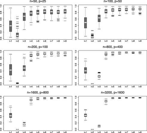
Figure 3: Boxplots for the ratios $\widehat{\lambda}_{i+1}/\widehat{\lambda}_{i}$ with two strong factors ($\delta=0$) and one weak factor ($\delta=0.5$) and $r=3$, $p=n/2$.

We also experiment with a setting with two strong factors (with $\delta=0$) and one weak factor (with $\delta=0.5$). Then the ratio-based estimator $\widehat{r}$ tends to take two values, picking up the two strong factors only. However Figure 3 indicates that the information on the third weak factor is not lost. In fact, $\widehat{\lambda}_{i+1}/\widehat{\lambda}_{i}$ tends to take the second smallest value at $i=3$. In this case a two-step estimation procedure should be employed in order to identify the number of factors correctly; see Section 4 below.

3.4 Improved rates for the estimated eigenvalues

The rates in Theorem 1 can be further improved, if we are prepared to entertain some additional conditions on $\bolds\varepsilon_{t}$ in model (1). Such an improvement is relevant as the condition that $h_{n}=p^{\delta}n^{-1/2}\to 0$, required in Theorem 1, is sometimes unnecessary. For example, in Table 1, the ratio-based estimator $\widehat{r}$ works perfectly well when $\delta=0.5$ and $n$ is sufficiently large (e.g., $n\geq 800$), even though $h_{n}=(p/n)^{1/2}\not\to 0$. Furthermore, in relation to the phenomenon of “blessing of dimensionality” exhibited in Table 1, Theorem 1 fails to reflect the possible improvement on the estimation for $r$ when $p$ increases; see also Remark 2(i). We first introduce some additional conditions on $\bolds\varepsilon_{t}$: [(C7)]

Let $\varepsilon_{jt}$ denote the $j$th component of $\bolds\varepsilon_{t}$. Then $\varepsilon_{jt}$ are independent for different $t$ and $j$, and have mean 0 and common variance $\sigma^{2}<\infty$.

The distribution of each $\varepsilon_{jt}$ is symmetric. Furthermore, $E(\varepsilon_{jt}^{2k+1})=0$, and $E(\varepsilon_{jt}^{2k})\leq(\tau k)^{k}$ for all $1\leq j\leq p$ and $t,k\geq 1$, where $\tau>0$ is a constant independent of $j,t,k$.

All the eigenvalues of $\bolds{\Sigma}_{\bolds\varepsilon}$ are uniformly bounded as $p\rightarrow\infty$. The moment condition $E(\varepsilon_{jt}^{2k})\leq(\tau k)^{k}$ in (C8) implies that $\varepsilon_{jt}$ are sub-Gaussian. Condition (C9) imposes some constraint on the correlations among the components of $\bolds\varepsilon_{t}$. When all components of $\{\bolds\varepsilon_{t}\}$ are independent $N(0,\sigma^{2})$, (C7)–(C9) hold. See also conditions (i^′)–(iv^′) of P09 .

Theorem 2

Let conditions (C1)–(C8) hold, $\ell_{n}\equiv p^{\delta/2}n^{-1/2}\to 0$ and $n=O(p)$. Then as $p,n\to\infty$, the following assertions hold:

$|\widehat{\lambda}_{j}-\lambda_{j}|=O_{P}(p^{2-3\delta/2}n^{-1/2})$ for $j=1,\ldots,r$,

$\widehat{\lambda}_{j}=O_{P}(p^{2-\delta}n^{-1})$ for $j=r+1,\ldots,(k_{0}+1)r$,

$\widehat{\lambda}_{j}=O_{P}(p^{2}n^{-2})$ for $j=(k_{0}+1)r+1,\ldots,p$.

If in addition (C9) holds, the rate in (ii) above can be further improved to

$$\widehat{\lambda}_{j}=O_{P}(p^{3/2-\delta}n^{-1/2}),\qquad j=r+1,\ldots,(k_{0}+1)r.$$ (13)

Corollary 2

Under the conditions of Theorem 2, it holds that

$$\widehat{\lambda}_{j+1}/\widehat{\lambda}_{j}\asymp 1,\qquad j=1,\ldots,r-1\mbox{,\quad and }\quad\widehat{\lambda}_{r+1}/\widehat{\lambda}_{r}=O_{P}(p^{\delta}n^{-1}).$$

If in addition (C9) also holds, $\widehat{\lambda}_{r+1}/\widehat{\lambda}_{r}=O_{P}(p^{\delta-1/2}n^{-1/2})$.

The proofs of Theorem 2 and Corollary 1 are given in the Appendix.

Remark 3.

(i) By comparing with Theorem 1, the error rate for nonzero $\lambda_{j}$ in Theorem 2 is improved by a factor $p^{-\delta/2}$, the error rate for zero-eigenvalues is by a factor $p^{-\delta}$ at least. However, those estimators themselves may still diverge, as illustrated in Figure 1.

(ii) Theorem 2(iii) is an interesting consequence of the random matrix theory. The key message here is as follows: for the eigenvalues corresponding purely to the matrix $\sum_{k=1}^{k_{0}}\widehat{\bolds}{\Sigma}_{\varepsilon}(k)\widehat{\bolds}{\Sigma}_{\varepsilon}(k)^{\prime}$, their magnitudes adjusted for $p^{2-2\delta}$ converge at a super-fast rate. The matrix $\sum_{k=1}^{k_{0}}\widehat{\bolds}{\Sigma}_{\varepsilon}(k)\widehat{\bolds}{\Sigma}_{\varepsilon}(k)^{\prime}$ is a part of $\widehat{\mathbf{M}}$ in (7), where $\widehat{\bolds}{\Sigma}_{\varepsilon}(k)$ is the sample lag-$k$ autocovariance matrix for $\{\bolds\varepsilon_{t}\}$. In particular, when all the factors are strong (i.e., $\delta=0$), the convergence rate is $n^{-2}$. Such a super convergence rate never occurs when $p$ is fixed.

(iii) Condition $\ell_{n}\to 0$ is mild, and is weaker than condition $h_{n}\to 0$ required in Theorem 1. For example, when $p\asymp n$, this condition is implied by the condition $\delta\in[0,1)$.

(iv) With additional condition (C9), $\widehat{\lambda}_{r+1}/\widehat{\lambda}_{r}=O_{P}(p^{-1/2}n^{-1/n})$ when all factors are strong. This shows that the speed at which $\widehat{\lambda}_{r+1}/\widehat{\lambda}_{r}$ converges to 0 increases when $p$ increases. This property gives a theoretical explanation why the identification for $r$ becomes easier for larger $p$ when all factors are strong (i.e., $\delta=0$). See Table 1.

4 Two-step estimation

In this section, we outline a two-step estimation procedure. We will show that it is superior than the one-step procedure presented in Section 2.2 for the determination of the number of factors as well as for the estimation of the factor loading matrices in the presence of the factors with different degrees of strength. A similar procedure is described in PP06 to improve the estimation for factor loading matrices in the presence of small eigenvalues, although they gave no theoretical underpinning on why and when such a procedure is advantageous.

Consider model (1) with $r_{1}$ strong factors with strength $\delta_{1}=0$ and $r_{2}$ weak factors with strength $\delta_{2}>0$, where $r_{1}+r_{2}=r$. Now (1) may be written as

$${\mathbf{y}}_{t}={\mathbf{A}}{\mathbf{x}}_{t}+\bolds\varepsilon_{t}={\mathbf{A}}_{1}{\mathbf{x}}_{1t}+{\mathbf{A}}_{2}{\mathbf{x}}_{2t}+\bolds\varepsilon_{t},$$ (14)

where ${\mathbf{x}}_{t}=({\mathbf{x}}_{1t}^{\prime}\enskip{\mathbf{x}}_{2t}^{\prime})^{\prime}$, ${\mathbf{A}}=({\mathbf{A}}_{1}\enskip{\mathbf{A}}_{2})$ with ${\mathbf{A}}^{\prime}{\mathbf{A}}={\mathbf{I}}_{r}$, ${\mathbf{x}}_{1t}$ consists of $r_{1}$ strong factors, and ${\mathbf{x}}_{2t}$ consists of $r_{2}$ weak factors. Like model (1) in Section 2.1, ${\mathbf{A}}=({\mathbf{A}}_{1},{\mathbf{A}}_{2})$ and ${\mathbf{x}}_{t}=({\mathbf{x}}_{1t},{\mathbf{x}}_{2t})$ are not uniquely defined, but only ${\mathcal{M}}({\mathbf{A}})$ is. Hereafter ${\mathbf{A}}=({\mathbf{A}}_{1},{\mathbf{A}}_{2})$ corresponds to a suitably rotated version of the original ${\mathbf{A}}$ in model (14), where now ${\mathbf{A}}$ contains all the eigenvectors of ${\mathbf{M}}$ corresponding to its nonzero eigenvalues. Refer to (6) for the definition of ${\mathbf{M}}$.

To present the two-step estimation procedure clearly, let us assume that we know $r_{1}$ and $r_{2}$ first. Using the method in Section 2.2, we first obtain the estimator $\widehat{\mathbf{A}}\equiv(\widehat{\mathbf{A}}_{1},\widehat{\mathbf{A}}_{2})$ for the factor loading matrix ${\mathbf{A}}=({\mathbf{A}}_{1},{\mathbf{A}}_{2})$, where the columns of $\widehat{\mathbf{A}}_{1}$ are the $r_{1}$ orthonormal eigenvectors of $\widehat{\mathbf{M}}$ corresponding to its $r_{1}$ largest eigenvalues. In practice we may identify $r_{1}$ using, for example, the ratio-based estimation method (8); see Figure 3. We carry out the second-step estimation as follows. Let

$${\mathbf{y}}_{t}^{*}={\mathbf{y}}_{t}-\widehat{\mathbf{A}}_{1}\widehat{\mathbf{A}}_{1}^{\prime}{\mathbf{y}}_{t}$$ (15)

for all $t$. We perform the same estimation for data $\{{\mathbf{y}}_{t}^{*}\}$ now, and obtain the $p\times r_{2}$ estimated factor loading matrix $\widetilde{\mathbf{A}}_{2}$ for the $r_{2}$ weak factors. Combining the two estimators together, we obtain the final estimator for ${\mathbf{A}}$ as

$$\widetilde{\mathbf{A}}=(\widehat{\mathbf{A}}_{1},\widetilde{\mathbf{A}}_{2}).$$ (16)

Theorem 3 below presents the convergence rates for both the one-step estimator $\widehat{\mathbf{A}}=(\widehat{\mathbf{A}}_{1},\widehat{\mathbf{A}}_{2})$ and the two-step estimator $\widetilde{\mathbf{A}}=(\widehat{\mathbf{A}}_{1},\widetilde{\mathbf{A}}_{2})$. It shows that $\widetilde{\mathbf{A}}$ converges to ${\mathbf{A}}$ at a faster rate than $\widehat{\mathbf{A}}$. The results are established with known $r_{1}$ and $r_{2}$. In practice we estimate $r_{1}$ and $r_{2}$ using the ratio-based estimators. See also Theorem 4 below. We introduce some regularity conditions first. Let $\bolds{\Sigma}_{12}(k)=\operatorname{Cov}({\mathbf{x}}_{1,t+k},{\mathbf{x}}_{2t})$, $\bolds{\Sigma}_{21}(k)=\operatorname{Cov}({\mathbf{x}}_{2,t+k},{\mathbf{x}}_{1t})$, $\bolds{\Sigma}_{i}(k)=\operatorname{Cov}({\mathbf{x}}_{i,t+k},{\mathbf{x}}_{it})$ and $\bolds{\Sigma}_{i\epsilon}(k)=\operatorname{Cov}({\mathbf{x}}_{i,t+k},\bolds\varepsilon_{t})$ for $i=1,2$: [(C6)^′]

For $i=1,2$, $1\leq k\leq k_{0}$, $\|\bolds{\Sigma}_{i}(k)\|\asymp p^{1-\delta_{i}}\asymp\|\bolds{\Sigma}_{i}(k)\|_{\min}$, $\|\bolds{\Sigma}_{21}(k)\|\asymp\|\bolds{\Sigma}_{21}(k)\|_{\min}$ and $\|\bolds{\Sigma}_{12}(k)\|=O(p^{1-\delta_{2}/2})$.

$\operatorname{Cov}({\mathbf{x}}_{t},{\varepsilon}_{s})=0$ for any $t,s$. The condition on $\bolds{\Sigma}_{i}(k)$ in (C5)^′ is an analogue to condition (C5). See Remark 1(i) in Section 3.2 for the background of those conditions. The order of $\|\bolds{\Sigma}_{21}(k)\|_{\min}$ will be specified in the theorems below. The order of $\|\bolds{\Sigma}_{12}(k)\|$ is not restrictive, since $p^{1-\delta_{2}/2}$ is the largest possible order when $\delta_{1}=0$. See also the discussion in Remark 1(ii). Condition (C6)^′ replaces condition (C6). Here we impose a strong condition $\bolds{\Sigma}_{i\epsilon}(k)=0$ to highlight the benefits of the two-step estimation procedure. See Remark 4(iii) below. Put

$${\mathbf{W}}_{i}=(\bolds{\Sigma}_{i}(1),\ldots,\bolds{\Sigma}_{i}(k_{0})),\qquad{\mathbf{W}}_{21}=(\bolds{\Sigma}_{21}(1),\ldots,\bolds{\Sigma}_{21}(k_{0})).$$

Theorem 3

Let conditions (C1)–(C4), (C5)^′, (C6)^′, (C7) and (C8) hold. Let $n=O(p)$ and $\kappa_{n}\equiv p^{\delta_{2}/2}n^{-1/2}\to 0$, as $n\to\infty$. Then it holds that

$$\|\widehat{\mathbf{A}}_{1}-{\mathbf{A}}_{1}\|=O_{P}(n^{-1/2}),\qquad\|\widetilde{\mathbf{A}}_{2}-{\mathbf{A}}_{2}\|=O_{P}(\kappa_{n})=\|\widetilde{\mathbf{A}}-{\mathbf{A}}\|.$$

Furthermore,

$$\|\widehat{\mathbf{A}}_{2}-{\mathbf{A}}_{2}\|=O_{P}(\nu_{n})=\|\widehat{\mathbf{A}}-{\mathbf{A}}\|,$$

if, in addition, $\nu_{n}\to 0$ and $p^{c\delta_{2}}n^{-1/2}\to 0$, where $\nu_{n}$ and $c$ are defined as follows:

$$\nu_{n}=\cases{p^{\delta_{2}}\kappa_{n},&\quad if $\|{\mathbf{W}}_{21}\|_{\min}=o(p^{1-\delta_{2}})$ $(c=1)$;\vspace*{2pt}\cr p^{(2c-1)\delta_{2}}\kappa_{n},&\quad if $\|{\mathbf{W}}_{21}\|_{\min}\asymp p^{1-c\delta_{2}}$ for $1/2\leq c<1$, and\vspace*{2pt}\cr&\quad$\|{\mathbf{W}}_{1}{\mathbf{W}}_{21}^{\prime}\|\leq q\|{\mathbf{W}}_{1}\|_{\min}\|{\mathbf{W}}_{21}\|$ for $0\leq q<1$.}$$

Note that $\kappa_{n}/\nu_{n}\to 0$. Theorem 3 indicates that between ${\mathbf{A}}_{1}$ and ${\mathbf{A}}_{2}$, the latter is more difficult to estimate, and the convergence rate of an estimator for ${\mathbf{A}}$ is determined by the rate for ${\mathbf{A}}_{2}$. This is intuitively understandable as the coefficient vectors for weak factors effectively contain many zero-components; see (9). Therefore a nontrivial proportion of the components of ${\mathbf{y}}_{t}$ may contain little information on weak factors. When $\|{\mathbf{W}}_{21}\|_{\min}\asymp p^{1-c\delta_{2}}$, $\|{\mathbf{W}}_{2}\|$ is dominated by $\|{\mathbf{W}}_{21}\|_{\min}$. The condition $\|{\mathbf{W}}_{1}{\mathbf{W}}_{21}^{\prime}\|\leq\break q\|{\mathbf{W}}_{1}\|_{\min}\|{\mathbf{W}}_{21}\|$ for $0\leq q<1$ is imposed to control the behavior of the $(r_{1}+1)$th to the $r$th largest eigenvalues of ${\mathbf{M}}$ under this situation. If this is not valid, those eigenvalues can become very small and give a bad estimator for ${\mathbf{A}}_{2}$, and thus ${\mathbf{A}}$. Under this condition, the structure of the autocovariance for the strong factors, and the structure of the cross-autocovariance between the strong and weak factors, are not similar.

Recall that $\lambda_{j}$ and $\widehat{\lambda}_{j}$ are the $j$th largest eigenvalue of, respectively, ${\mathbf{M}}$ defined in (6) and $\widehat{\mathbf{M}}$ defined in (7). We define matrices ${\mathbf{M}}^{*}$ and $\widehat{\mathbf{M}}^{*}$ in the same manner as ${\mathbf{M}}$ and $\widehat{\mathbf{M}}$ but with $\{{\mathbf{y}}_{t}\}$ replaced by $\{{\mathbf{y}}_{t}^{*}\}$ defined in (15), and denote by $\lambda_{j}^{*}$ and $\widehat{\lambda}_{j}^{*}$ the $j$th largest eigenvalue of, respectively, ${\mathbf{M}}^{*}$ and $\widehat{\mathbf{M}}^{*}$. The following theorem shows the different behavior of the ratio of eigenvalues under the one-step and two-step estimation. Readers who are interested in the explicit rates for the eigenvalues are referred to Lemma 1 in the Appendix.

Theorem 4

Under the same conditions of Theorem 3, the following assertions hold:

For $1\leq i<r_{1}$ or $r_{1}<i<r$, $\widehat{\lambda}_{i+1}/\widehat{\lambda}_{i}\asymp 1$. For $1\leq 1<r_{2}$, $\widehat{\lambda}^{*}_{j+1}/\widehat{\lambda}^{*}_{j}\asymp 1$.

$\widehat{\lambda}_{r+1}/\widehat{\lambda}_{r}\stackrel{{\scriptstyle P}}{{\longrightarrow}}0$ and $\widehat{\lambda}_{r_{1}+1}/\widehat{\lambda}_{r_{1}}=o_{p}(\widehat{\lambda}_{r+1}/\widehat{\lambda}_{r})$ provided

$$\delta_{2}>1/(8c-1),\qquad p^{(1-\delta_{2})/2}n^{-1/2}\to 0,\qquad p^{(6c-1/2)\delta_{2}-1/2}n^{-1/2}\to\infty.$$

$\widehat{\lambda}_{r+1}/\widehat{\lambda}_{r}\stackrel{{\scriptstyle P}}{{\longrightarrow}}0$ and $\widehat{\lambda}_{r_{2}+1}^{*}/\widehat{\lambda}^{*}_{r_{2}}=o_{p}(\widehat{\lambda}_{r+1}/\widehat{\lambda}_{r})$ provided $p^{(4c-3/2)\delta_{2}-1/2}\times\allowbreak n^{1/2}\rightarrow\infty$.

Remark 4.

(i) Theorem 4(i) and (ii) imply that the one-step estimation is likely to lead to $\widehat{r}=r_{1}$. For instance, when $p\asymp n$, then Theorem 4(ii) says that $\widehat{\lambda}_{r_{1}+1}/\widehat{\lambda}_{r_{1}}$ has a faster rate of convergence than $\widehat{\lambda}_{r+1}/\widehat{\lambda}_{r}$ as long as $\delta_{2}>2/5$. Figure 3 shows exactly this situation.

(ii) Theorem 4(iii) implies that the two-step estimation is more capable to identify the additional $r_{2}$ factors than the one-step estimation. In particular, if $p\asymp n$, $\widehat{\lambda}_{r_{2}+1}^{*}/\widehat{\lambda}^{*}_{r_{2}}$ always has a faster rate of convergence than $\widehat{\lambda}_{r+1}/\widehat{\lambda}_{r}$. Unfortunately we are unable to establish the asymptotic properties for $\widehat{\lambda}_{i+1}/\widehat{\lambda}_{i}$ for $i>r$, and $\widehat{\lambda}_{j+1}^{*}/\widehat{\lambda}_{j}^{*}$ for $j>r_{2}$, though we believe that conjectures similar to (11) continue to hold.

(iii) When $\delta_{1}>0$ and/or the cross-autocovariances between different factors and the noise are stronger, the similar and more complex results can be established via more involved algebra in the proofs.

5 Real data examples

We illustrate our method using two real data sets.

Example 1.

We first analyze the daily returns of 123 stocks in the period 2 January 2002–11 July 2008. Those stocks were selected among those included in the S&P500 and were traded every day during the period. The returns were calculated in percentages based on the daily close prices. We have in total $n=1642$ observations with $p=123$. We apply the eigenanalysis to the matrix $\widehat{\mathbf{M}}$ defined in (7) with $k_{0}=5$. The obtained eigenvalues (in descending order) and their ratios are plotted in Figure 4. It is clear that the ratio-based estimator (8) leads to $\widehat{r}=2$, indicating two factors.

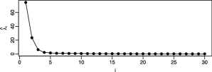
(a)

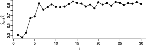
(b)

Figure 4: Plots of the estimated eigenvalues (a) and the ratios of estimated eigenvalues of $\widehat{\mathbf{M}}$ (b) for Example 1.

Varying the value of $k_{0}$ between 1 and 100 in the definition of $\widehat{\mathbf{M}}$ leads to little change in the ratios $\widehat{\lambda}_{i+1}/\widehat{\lambda}_{i}$, and the estimate $\widehat{r}=2$ remains unchanged. Figure 4(a) shows that $\widehat{\lambda}_{i}$ is close to 0 for all $i\geq 5$. Figure 4(b) indicates that the ratio $\widehat{\lambda}_{i+1}/\widehat{\lambda}_{i}$ is close to 1 for all large $i$, which is in line with conjecture (11).

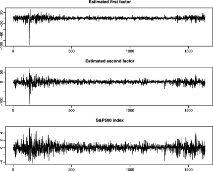
Figure 5: The time series plots of the two estimated factors and the return series of the S&P500 index in the same time period.

The first two panels of Figure 5 display the time series plots of the two component series of the estimated factors $\widehat{\mathbf{x}}_{t}$ defined as in (2). Their cross-autocorrelations are presented in Figure 6. Although each of the two estimated factors shows little significant autocorrelation, there are some significant cross-correlations between the two series. The cross-autocorrelations of the three residual series $\widehat{\bolds}{\gamma}_{j}^{\prime}{\mathbf{y}}_{t}$ for $j=3,4,5$ are not significantly different from 0, where $\widehat{\bolds}{\gamma}_{j}$ is the unit eigenvector of $\widehat{\mathbf{M}}$ corresponding to its $j$th largest eigenvalue. If there were any serial correlations left in the data after extracting the two estimated factors, those correlations are most likely to show up in those three residual series.

Figure 4 may suggest the existence of a third and weaker factor, though there are hardly any significant autocorrelations in the series $\widehat{\bolds}{\gamma}_{3}^{\prime}{\mathbf{y}}_{t}$. In fact $\widehat{\lambda}_{3}=6.231$ and $\widehat{\lambda}_{4}/\widehat{\lambda}_{3}=0.357$. Note that now $\widehat{\lambda}_{j}$ is not necessarily a consistent estimator for $\lambda_{j}$ although $\widehat{\lambda}_{r+1}/\widehat{\lambda}_{r}\stackrel{{\scriptstyle P}}{{\longrightarrow}}0$; see Theorem 1(ii) and Corollary 1. To investigate this further, we apply the two-step estimation procedure presented in Section 4. By subtracting the two estimated factors from the above, we obtain the new data ${\mathbf{y}}_{t}^{*}$ [see (16)]. We then calculate the eigenvalues and their ratios of the matrix $\widehat{\mathbf{M}}^{*}$. The minimum value of the ratios is $\widehat{\lambda}_{2}^{*}/\widehat{\lambda}_{1}^{*}=0.667$, which is closely followed by $\widehat{\lambda}_{3}^{*}/\widehat{\lambda}_{2}^{*}=0.679$ and $\widehat{\lambda}^{*}_{4}/\widehat{\lambda}_{3}^{*}=0.744$. There is no evidence to suggest that $\widehat{\lambda}_{2}^{*}/\widehat{\lambda}_{1}^{*}\to 0$; see Theorem 4. This reinforces our choice $\widehat{r}=2$.

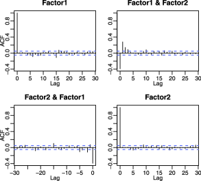
Figure 6: The cross-autocorrelations of the two estimated factors for Example 1.

With $p$ as large as 123, it is difficult to gain insightful interpretation on the estimated factors by looking through the coefficients in $\widehat{\mathbf{A}}$ [see (2)]. To link our fitted factor model with some classical asset pricing theory in finance, we wonder if the market index (i.e., the S&P500 index) is a factor in our fitted model, or more precisely, if it can be written as a linear combination of the two estimated factors. When this is true, ${\mathbf{P}}{\mathbf{u}}=0$, where ${\mathbf{u}}$ is the $1642\times 1$ vector consisting of the returns of the S&P500 index over the same time period, and ${\mathbf{P}}$ denotes the projection matrix onto the orthogonal complement of the linear space spanned by the two component series $\widehat{\mathbf{x}}_{t}$, which is a 1640-dimensional subspace in $R^{1642}$. This S&P500 return series is plotted together with the two component series $\widehat{\mathbf{x}}_{t}$ in Figure 5. It turns out that $\|{\mathbf{P}}{\mathbf{u}}\|^{2}$ is not exactly 0 but $\|{\mathbf{P}}{\mathbf{u}}\|^{2}/\|{\mathbf{u}}\|^{2}=0.023$, that is, the 97.7% of the S&P500 returns can be expressed as a linear combination of the two estimated factors. Thus our analysis suggests the following model for ${\mathbf{y}}_{t}$—the daily returns of the 123 stocks:

$${\mathbf{y}}_{t}={\mathbf{a}}_{1}u_{t}+{\mathbf{a}}_{2}v_{t}+\bolds\varepsilon_{t},$$

where $u_{t}$ denotes the return of the S&P500 on the day $t$, $v_{t}$ is another factor, and $\bolds\varepsilon_{t}$ is a $123\times 1$ vector white-noise process.

Figure 5 shows that there is an early period with big sparks in the two estimated factor processes. Those sparks occurred around 24 September 2002 when the markets were highly volatile and the Dow Jones Industrial Average had lost 27% of the value it held on 1 January 2001. However, those sparks are significantly less extreme in the returns of the S&P500 index; see the third panel in Figure 5. In fact the projected S&P500 return ${\mathbf{P}}{\mathbf{u}}$ is the linear combination of those two estimated factors with the coefficients ($-0.0548,0.0808$). Two observations may be drawn from the opposite signs of those two coefficients: (i) there is an indication that those two factors draw the energy from the markets with opposite directions, and (ii) the portfolio S&P500 index hedges the risks across different markets.

Example 2.

We analyze a set of monthly average sea surface air pressure records (in Pascal) from January 1958 to December 2001 (i.e., 528 months in total) over a $10\times 44$ grid in a range of $22.5^{\circ}$–$110^{\circ}$ longitude in the North Atlantic Ocean. Let $P_{t}(u,v)$ denote the air pressure in the $t$th month at the location $(u,v)$, where $u=1,\ldots,10,v=1,\ldots,44$ and $t=1,\ldots,528$. We first subtract each data point by the monthly mean over the 44 years at its location: $\frac{1}{44}\sum_{i=1}^{44}P_{12(i-1)+j}(u,v)$, where $j=1,\ldots,12$, representing the 12 different months over a year. We then line up the new data over $10\times 44=440$ grid points as a vector ${\mathbf{y}}_{t}$, so that ${\mathbf{y}}_{t}$ is a $p$-variate time series with $p=440$. We have $n=528$ observations.

To fit the factor model (1) to ${\mathbf{y}}_{t}$, we calculate the eigenvalues and the eigenvectors of the matrix $\widehat{\mathbf{M}}$ defined in (7) with $k_{0}=5$. Let $\widehat{\lambda}_{1}>\widehat{\lambda}_{2}>\cdots$ denote the eigenvalues of $\widehat{\mathbf{M}}$. The ratios $\widehat{\lambda}_{i+1}/\widehat{\lambda}_{i}$ are plotted against $i$ in the top panel of Figure 7 which indicates the ratio-based estimate for the number of factor is $\widehat{r}=1$; see (8). However, the second smallest ratio is $\widehat{\lambda}_{4}/\widehat{\lambda}_{3}$. This suggests that there may exist two weaker factors in addition; see Theorem 4(ii) and also Figure 3. We adopt the two-step estimation procedure presented in Section 4 to identify the factors of different strength. By removing the factor corresponding to the largest eigenvalue of $\widehat{\mathbf{M}}$,

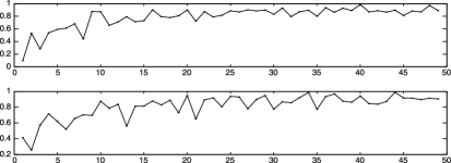
Figure 7: Plots of $\widehat{\lambda}_{i+1}/\widehat{\lambda}_{i}$—the ratio of the eigenvalues of $\widehat{\mathbf{M}}$ (the top panel) and $\widehat{\mathbf{M}}^{*}$ (the bottom panel), against $i$, for Example 2.

the resulting “residuals” are denoted as ${\mathbf{y}}_{t}^{*}$; see (15). Now we repeat the factor modeling for data ${\mathbf{y}}_{t}^{*}$, and plot the ratios of eigenvalues of matrix $\widehat{\mathbf{M}}^{*}$ in the second panel of Figure 7. It shows clearly the minimum value at 2, indicating further two (weaker) factors. Combining the above two steps together, we set $\widehat{r}=3$ in the fitted model. We repeated the above calculation with $k_{0}=1$ in (7). We still find three factors with the two-step procedure, and the estimated factors series are very similar to the case when $k_{0}=5$. This is consistent with the simulation results in LYB11 , where they showed empirically that the estimated factor models are not sensitive to the choice of $k_{0}$.

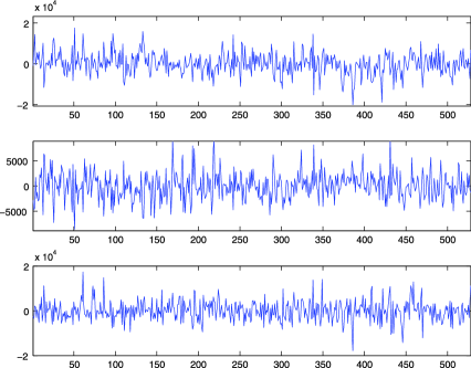
Figure 8: Time series plot of the three estimated factors for Example 2.

We present the time series plots for the three estimated factors $\widehat{\mathbf{x}}_{t}=\widetilde{\mathbf{A}}^{\prime}{\mathbf{y}}_{t}$ in Figure 8, where $\widetilde{\mathbf{A}}$ is a $440\times 3$ matrix with the first column being the unit eigenvector of $\widehat{\mathbf{M}}$ corresponding to its largest eigenvalue, and the other two columns being the orthonormal eigenvectors of $\widehat{\mathbf{M}}^{*}$ corresponding

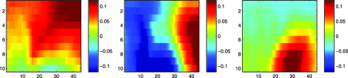
Figure 9: Factor loading surface of the first, second and third factors (from left to right) for Example 2.

to its two largest eigenvalues; see (16) and also (2). They collectively account for 85.3% of the total variation in ${\mathbf{y}}_{t}$ which has $440$ components. In fact each of the three factors accounts for, respectively, 57.5%, 18.2% and 9.7% of the total variation of ${\mathbf{y}}_{t}$. Figure 9 depicts the factor loading surfaces of the three factors. Some interesting regional patterns are observed from those plots. For example, the first factor is the main driving force for the dynamics in the north and especially the northeast. The second factor influences the dynamics in the east and the west in the opposite directions, and has little impact in the narrow void between them. The third factor impacts mainly the dynamics of the southeast region. We also notice that none of those factors can be seen as idiosyncratic components as each of them affects quite a large number of locations.

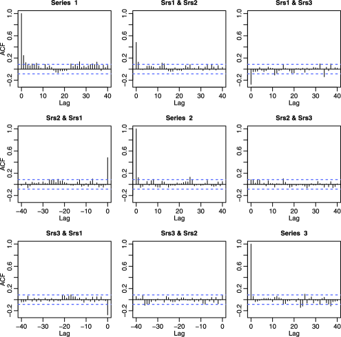
Figure 10: Example 2: sample cross-correlation functions for the three estimated factors.

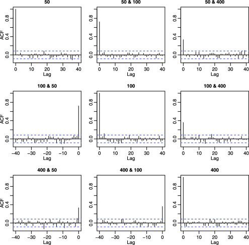
Figure 11: Example 2: sample cross-correlation functions for three residual series. 50 represents grid position (10, 5), 100 for (10, 10) and 400 for (10, 40).

Figure 10 presents the sample cross-correlations for the three estimated factors. It shows significant, though small, autocorrelations or cross-correlations at some nonzero lags. Figure 11 is the sample cross-correlations for three residuals series selected from three locations for which one is far apart from the other two spatially, showing little autocorrelations at nonzero lags. This indicates that our approach is capable to identify the factors based on serial correlations.

Finally we note that the BIC method of BN02 yields the estimate $\widehat{r}=n=528$ for this particular data set. We suspect that this may be due to the fact that BN02 requires all the eigenvalues of $\bolds{\Sigma}_{\varepsilon}$ be uniformly bounded when $p\to\infty$. This may not be the case for this particular data set, as the nearby locations are strongly spatially correlated, which may lead to very large and also very small eigenvalues for $\bolds{\Sigma}_{\varepsilon}$. Indeed, for this data set, the three largest eigenvalues of $\widehat{\bolds}{\Sigma}_{\varepsilon}$ are on the order of $10^{6}$, and the three smallest eigenvalues are practically 0. Since the typical magnitude of $\widehat{\bolds}\varepsilon_{t}$ is $10^{2}$ from our analysis, we have done simulations (not shown here) showing that the typical largest eigenvalues for $\widehat{\bolds}{\Sigma}_{{\varepsilon}}$, if $\{\bolds\varepsilon_{t}\}$ is weakly correlated white noise, should be around $10^{4}$ to $10^{5}$, and the smallest around $10^{2}$ to $10^{3}$ when $p=440$ and $n=528$. Such a huge difference in the magnitude of the eigenvalues suggests strongly that the components of the white-noise vector $\bolds\varepsilon_{t}$ are strongly correlated. Our method does not require the uniform boundedness of the eigenvalues of $\bolds{\Sigma}_{{\varepsilon}}$.

Appendix

Proof of Theorem 1 We present some notational definitions first. We denote by $\widehat{\lambda}_{j},\widehat{\bolds}{\gamma}_{j}$ the $j$th largest eigenvalue of $\widehat{\mathbf{M}}$ and the corresponding orthonormal eigenvector, respectively. The corresponding population values are denoted by $\lambda_{j}$ and ${\mathbf{a}}_{j}$ for the matrix ${\mathbf{M}}$. Hence $\widehat{\mathbf{A}}=(\widehat{\bolds}{\gamma}_{1},\ldots,\widehat{\bolds}{\gamma}_{r})$ and ${\mathbf{A}}=({\mathbf{a}}_{1},\ldots,{\mathbf{a}}_{r})$. We also have

$$\lambda_{j}={\mathbf{a}}_{j}^{\prime}{\mathbf{M}}{\mathbf{a}}_{j},\qquad\widehat{\lambda}_{j}=\widehat{\bolds}{\gamma}_{j}^{\prime}\widehat{\mathbf{M}}\widehat{\bolds}{\gamma}_{j},\qquad j=1,\ldots,p.$$

We show some intermediate results now. With conditions (C3) and (C5) and the fact that $\{\bolds\varepsilon_{t}\}$ is white noise, we have

$$\|\widehat{\bolds}{\Sigma}_{x}(k)-\bolds{\Sigma}_{x}(k)\| = O_{P}(p^{1-\delta}n^{-1/2}),$$

$$\|\widehat{\bolds}{\Sigma}_{x\epsilon}(k)-\bolds{\Sigma}_{x\epsilon}(k)\|,\qquad\|\widehat{\bolds}{\Sigma}_{\epsilon x}(k)\| = O_{P}(p^{1-\delta/2}n^{-1/2}),$$

where $k=0,1,\ldots,k_{0}$. Then following the proof of Theorem 1 of LYB11 , we have the following for $k=1,\ldots,k_{0}$:

$$\|\widehat{\mathbf{M}}-{\mathbf{M}}\|=O_{P}\bigl{(}\|\bolds{\Sigma}_{y}(k)\|\cdot\|\widehat{\bolds}{\Sigma}_{y}(k)-\bolds{\Sigma}_{y}(k)\|\bigr{)}$$

$$\qquad\mbox{where }\hskip 40.5pt\|\bolds{\Sigma}_{y}(k)\|=O(p^{1-\delta}),$$

$$\qquad\hphantom{\mbox{where }}\|\widehat{\bolds}{\Sigma}_{y}(k)-\bolds{\Sigma}_{y}(k)\|=O_{P}\bigl{(}p^{1-\delta}n^{-1/2}+p^{1-\delta/2}n^{-1/2}+\|\widehat{\bolds}{\Sigma}_{\epsilon}(k)\|\bigr{)}$$

$$\qquad\hphantom{\mbox{where }\|\widehat{\bolds}{\Sigma}_{y}(k)-\bolds{\Sigma}_{y}(k)\|}=O_{P}\bigl{(}p^{1-\delta/2}n^{-1/2}+\|\widehat{\bolds}{\Sigma}_{\epsilon}(k)\|\bigr{)}.$$

Now $\|\widehat{\bolds}{\Sigma}_{\epsilon}(k)\|\leq\|\widehat{\bolds}{\Sigma}_{\epsilon}(k)\|_{F}=O_{P}(pn^{-1/2})$, where $\|{\mathbf{M}}\|_{F}=\operatorname{trace}({\mathbf{M}}{\mathbf{M}}^{\prime})$ denotes the Frobenius norm of ${\mathbf{M}}$. Hence from (Appendix),

$$\|\widehat{\bolds}{\Sigma}_{y}(k)-\bolds{\Sigma}_{y}(k)\| = O_{P}(pn^{-1/2})\quad\mbox{and }$$

$$\|\widehat{\mathbf{M}}-{\mathbf{M}}\| = O_{P}(p^{1-\delta}\cdot pn^{-1/2})=O_{P}(p^{2-\delta}n^{-1/2}).$$

For the main proof, consider for $j=1,\ldots,r$, the decomposition

$$\widehat{\lambda}_{j}-\lambda_{j}=\widehat{\bolds}{\gamma}_{j}^{\prime}\widehat{\mathbf{M}}\widehat{\bolds}{\gamma}_{j}-{\mathbf{a}}_{j}^{\prime}{\mathbf{M}}{\mathbf{a}}_{j}=I_{1}+I_{2}+I_{3}+I_{4}+I_{5}$$

$$\qquad\mbox{where }I_{1}=(\widehat{\bolds}{\gamma}_{j}-{\mathbf{a}}_{j})^{\prime}(\widehat{\mathbf{M}}-{\mathbf{M}})\widehat{\bolds}{\gamma}_{j},\qquad I_{2}=(\widehat{\bolds}{\gamma}_{j}-{\mathbf{a}}_{j})^{\prime}{\mathbf{M}}(\widehat{\bolds}{\gamma}_{j}-{\mathbf{a}}_{j}),$$

$$\qquad\hphantom{\mbox{where }}I_{3}=(\widehat{\bolds}{\gamma}_{j}-{\mathbf{a}}_{j})^{\prime}{\mathbf{M}}{\mathbf{a}}_{j},\qquad I_{4}={\mathbf{a}}_{j}^{\prime}(\widehat{\mathbf{M}}-{\mathbf{M}})\widehat{\bolds}{\gamma}_{j},$$

$$\qquad\hphantom{\mbox{where }}I_{5}={\mathbf{a}}_{j}^{\prime}{\mathbf{M}}(\widehat{\bolds}{\gamma}_{j}-{\mathbf{a}}_{j}).$$

For $j=1,\ldots,r$, since $\|\widehat{\bolds}{\gamma}_{j}-{\mathbf{a}}_{j}\|\leq\|\widehat{\mathbf{A}}-{\mathbf{A}}\|=O_{P}({h_{n}})$ where $h_{n}=p^{\delta}n^{-1/2}$, and $\|{\mathbf{M}}\|\leq\sum_{k=1}^{k_{0}}\|\bolds{\Sigma}_{y}(k)\|^{2}=O_{P}(p^{2-2\delta})$ by (Appendix), together with (Appendix) we have that

$$\|I_{1}\|,\|I_{2}\|=O_{P}(p^{2-2\delta}h_{n}^{2}),\qquad\|I_{3}\|,\|I_{4}\|,\|I_{5}\|=O_{P}(p^{2-2\delta}h_{n}),$$

so that $|\widehat{\lambda}_{j}-\lambda_{j}|=O_{P}(p^{2-2\delta}h_{n})=O_{P}(p^{2-\delta}n^{-1/2})$, which proves Theorem 1(i).

Now consider $j=r+1,\ldots,p$. Define

$$\widetilde{\mathbf{M}}=\sum_{k=1}^{k_{0}}\widehat{\bolds}{\Sigma}_{y}(k)\bolds{\Sigma}_{y}(k)^{\prime},\qquad\widehat{\mathbf{B}}=(\widehat{\bolds}{\gamma}_{r+1},\ldots,\widehat{\bolds}{\gamma}_{p}),\qquad{\mathbf{B}}=({\mathbf{a}}_{r+1},\ldots,{\mathbf{a}}_{p}).$$

Following the same proof of Theorem 1 of LYB11 , we can actually show that $\|\widehat{\mathbf{B}}-{\mathbf{B}}\|=O_{P}(h_{n})$, so that $\|\widehat{\bolds}{\gamma}_{j}-{\mathbf{a}}_{j}\|\leq\|\widehat{\mathbf{B}}-{\mathbf{B}}\|=O_{P}(h_{n})$.

Noting $\lambda_{j}=0$ for $j=r+1,\ldots,p$, consider the decomposition

$$\widehat{\lambda}_{j}=\widehat{\bolds}{\gamma}_{j}^{\prime}\widehat{\mathbf{M}}\widehat{\bolds}{\gamma}_{j}=K_{1}+K_{2}+K_{3}$$

$$\qquad\mbox{where }K_{1}=\widehat{\bolds}{\gamma}_{j}^{\prime}(\widehat{\mathbf{M}}-\widetilde{\mathbf{M}}-\widetilde{\mathbf{M}}^{\prime}+{\mathbf{M}})\widehat{\bolds}{\gamma}_{j},$$

(21)

$$\hphantom{\qquad\mbox{where }}K_{2}=2\widehat{\bolds}{\gamma}_{j}^{\prime}(\widetilde{\mathbf{M}}-{\mathbf{M}})(\widehat{\bolds}{\gamma}_{j}-{\mathbf{a}}_{j}),$$

$$\hphantom{\qquad\mbox{where }}K_{3}=(\widehat{\bolds}{\gamma}_{j}-{\mathbf{a}}_{j})^{\prime}{\mathbf{M}}(\widehat{\bolds}{\gamma}_{j}-{\mathbf{a}}_{j}).$$

Using (Appendix),

$$K_{1}=\sum_{k=1}^{k_{0}}\bigl{\|}\bigl{(}\widehat{\bolds}{\Sigma}_{y}(k)-\bolds{\Sigma}_{y}(k)\bigr{)}^{\prime}\widehat{\bolds}{\gamma}_{j}\bigr{\|}^{2}\leq\sum_{k=1}^{k_{0}}\|\widehat{\bolds}{\Sigma}_{y}(k)-\bolds{\Sigma}_{y}(k)\|^{2}=O_{P}(p^{2}n^{-1}).$$

Similarly, using (Appendix) and (Appendix), and $\|\widehat{\mathbf{B}}-{\mathbf{B}}\|=O_{P}(h_{n})$, we can show that

$$|K_{2}| = O_{P}(\|\widetilde{\mathbf{M}}-{\mathbf{M}}\|\cdot\|\widehat{\bolds}{\gamma}_{j}-{\mathbf{a}}_{j}\|)=O_{P}(\|\widehat{\mathbf{M}}-{\mathbf{M}}\|\cdot\|\widehat{\mathbf{B}}-{\mathbf{B}}\|)=O_{P}(p^{2}n^{-1}),$$

$$|K_{3}| = O_{P}(\|\widehat{\mathbf{B}}-{\mathbf{B}}\|^{2}\cdot\|{\mathbf{M}}\|)=O_{P}(p^{2-2\delta}h_{n}^{2})=O_{P}(p^{2}n^{-1}).$$

Hence $\widehat{\lambda}_{j}=O_{P}(p^{2}n^{-1})$, and the proof of the theorem is completed. Proof of Corollary 1 The proof of Theorem 1 of LYB11 has shown that (in the notation of this paper)

$$p^{2-2\delta}=O(\lambda_{r}).$$

But we also have

$$\lambda_{r}\leq\lambda_{1}=\|{\mathbf{M}}\|\leq\sum_{k=1}^{k_{0}}\|\bolds{\Sigma}_{y}(k)\|^{2}=O(p^{2-2\delta}),$$

where the last equality sign follows from $\|\bolds{\Sigma}_{y}(k)\|=O(p^{1-\delta})$ in (Appendix). Hence we have $\lambda_{i}\asymp p^{2-2\delta}$ for $i=1,\ldots,r$.

Letting $e_{i}=|\widehat{\lambda}_{i}-\lambda_{i}|$ for $i=1,\ldots,r$, we then have $e_{i}=O_{P}(p^{2-\delta}n^{-1/2})$ from Theorem 1(i). But since $h_{n}=p^{\delta}n^{-1/2}=o(1)$ implying that $p^{2-\delta}n^{-1/2}=p^{2-2\delta}h_{n}=o(p^{2-2\delta})$, we have $e_{i}=o_{P}(\lambda_{i})$. Hence we must have $\widehat{\lambda}_{i}\asymp\lambda_{i}\asymp p^{2-2\delta}$ for $i=1,\ldots,r$. This implies that $\widehat{\lambda}_{j+1}/\widehat{\lambda}_{j}\asymp 1$ for $j=1,\ldots,r-1$, and together with Theorem 1(ii),

$$\widehat{\lambda}_{r+1}/\widehat{\lambda}_{r}=O_{P}(p^{2}n^{-1}/p^{2-2\delta})=O_{P}(p^{2\delta}n^{-1})=O_{P}(h_{n}^{2}).$$

This completes the proof of the corollary.

In the following, we use $\sigma_{j}({\mathbf{M}})$ to denote the $j$th largest singular value of a matrix ${\mathbf{M}}$, so that $\sigma_{1}({\mathbf{M}})=\|{\mathbf{M}}\|$. We use $\lambda_{j}({\mathbf{M}})$ to denote the $j$th largest eigenvalue of ${\mathbf{M}}$. Proof of Theorem 2 The first part of the theorem is actually Theorem 2 of LYB11 . We prove the other parts of the theorem. From equation (22) of LYB11 , the sample lag-$k$ autocovariance matrix for $\bolds\varepsilon_{t}$ satisfies

$$\|\widehat{\bolds}{\Sigma}_{\epsilon}(k)\|=O_{P}(pn^{-1}).$$ (22)

Note that (Appendix) together with (22) implies

$$\|\widehat{\mathbf{M}}-{\mathbf{M}}\| = O_{P}\bigl{(}p^{1-\delta}(p^{1-\delta/2}n^{-1/2}+pn^{-1})\bigr{)}$$

$$= O_{P}\bigl{(}p^{2-2\delta}(p^{\delta/2}n^{-1/2}+p^{\delta}n^{-1})\bigr{)}=O_{P}(p^{2-2\delta}\ell_{n}),$$

since $\ell_{n}=p^{\delta/2}n^{-1/2}=o(1)$. We also have $\|\widehat{\mathbf{B}}-{\mathbf{B}}\|=O_{P}(\ell_{n})$, similar to the proof of Theorem 1.

With these, for $j=1,\ldots,r$, using decomposition (Appendix), we have

$$|\widehat{\lambda}_{j}-\lambda_{j}|=O_{P}(\|\widehat{\mathbf{M}}-{\mathbf{M}}\|)=O_{P}(p^{2-2\delta}\ell_{n})=O_{P}(p^{2-3\delta/2}n^{-1/2}),$$

which is Theorem 2(i). For $j=r+1,\ldots,(k_{0}+1)r$, using decomposition (Appendix), we have

$$K_{1} = O_{P}\bigl{(}(p^{1-\delta/2}n^{-1/2}+pn^{-1})^{2}\bigr{)}=O_{P}(p^{2-\delta}n^{-1}+p^{2}n^{-2})=O_{P}(p^{2-\delta}n^{-1}),$$

$$|K_{2}| = O_{P}(\|\widehat{\mathbf{M}}-{\mathbf{M}}\|\cdot\|\widehat{\mathbf{B}}-{\mathbf{B}}\|)=O_{P}(p^{2-2\delta}\ell_{n}^{2})=O_{P}(p^{2-\delta}n^{-1}),$$

$$|K_{3}| = O_{P}(\|\widehat{\mathbf{B}}-{\mathbf{B}}\|^{2}\cdot\|{\mathbf{M}}\|)=O_{P}(p^{2-2\delta}\ell_{n}^{2})=O_{P}(p^{2-\delta}n^{-1}).$$

Hence $\widehat{\lambda}_{j}=O_{P}(p^{2-2\delta}\ell_{n}^{2})=O_{P}(p^{2-\delta}n^{-1})$, which is Theorem 2(ii).

For part (iii), we define

$${\mathbf{W}}_{y}(k_{0})=(\bolds{\Sigma}_{y}(1),\ldots,\bolds{\Sigma}_{y}(k_{0})),\qquad\widehat{\mathbf{W}}_{y}(k_{0})=(\widehat{\bolds}{\Sigma}_{y}(1),\ldots,\widehat{\bolds}{\Sigma}_{y}(k_{0})),$$

so that ${\mathbf{M}}={\mathbf{W}}_{y}(k_{0}){\mathbf{W}}_{y}(k_{0})^{\prime}$ and $\widehat{\mathbf{M}}=\widehat{\mathbf{W}}_{y}(k_{0})\widehat{\mathbf{W}}_{y}(k_{0})^{\prime}$. We define similarly $\widehat{\mathbf{W}}_{x}(k_{0}),\widehat{\mathbf{W}}_{x\epsilon}(k_{0})$, $\widehat{\mathbf{W}}_{\epsilon x}(k_{0})$ and $\widehat{\mathbf{W}}_{\epsilon}(k_{0})$. Then we can write

$$\widehat{\mathbf{W}}_{y}(k_{0})=M_{1}+M_{2}+\widehat{\mathbf{W}}_{\epsilon}(k_{0}),$$

where $M_{1}={\mathbf{A}}(\widehat{\mathbf{W}}_{x}(k_{0})({\mathbf{I}}_{k_{0}}\otimes{\mathbf{A}}^{\prime})+\widehat{\mathbf{W}}_{x\epsilon}(k_{0}))$, $M_{2}=\widehat{\mathbf{W}}_{\epsilon x}(k_{0})({\mathbf{I}}_{k_{0}}\otimes{\mathbf{A}}^{\prime})$. It is easy to see that

$$\operatorname{rank}(M_{1})\leq r,\qquad\operatorname{rank}(M_{2})\leq k_{0}r,$$

so that rank$(M_{1}+M_{2})\leq(k_{0}+1)r$. This implies that

$$\sigma_{j}(M_{1}+M_{2})=0\qquad\mbox{for }j=(k_{0}+1)r+1,\ldots,p.$$

Then by Theorem 3.3.16(a) of HJ91 , for $j=(k_{0}+1)r+1,\ldots,p$,

$$\widehat{\lambda}_{j} = \lambda_{j}(\widehat{\mathbf{M}})=\sigma_{j}^{2}(\widehat{\mathbf{W}}_{y}(k_{0}))\leq\bigl{(}\sigma_{j}(M_{1}+M_{2})+\sigma_{1}(\widehat{\mathbf{W}}_{\epsilon}(k_{0}))\bigr{)}^{2}$$

$$= \sigma_{1}^{2}(\widehat{\mathbf{W}}_{\epsilon}(k_{0}))\leq\sum_{k=1}^{k_{0}}\|\widehat{\bolds}{\Sigma}_{\epsilon}(k)\|^{2}=O_{P}(p^{2}n^{-2}),$$

where the last equality sign follows from (22). This proves Theorem 2(iii).

We prove Theorem 2(ii)^′ now. Using Lemma 3 of LYB11 , with the same technique as in the proof of Theorem 1 in their paper, we can write

$$\widehat{\mathbf{B}}=({\mathbf{B}}+{\mathbf{A}}{\mathbf{P}})({\mathbf{I}}+{\mathbf{P}}^{\prime}{\mathbf{P}})^{-1/2}\qquad\mbox{with }\|{\mathbf{P}}\|=O_{P}(\ell_{n}).$$ (23)

With the definition of $\widehat{\mathbf{B}}$ as in the proof of Theorem 1, we can write $\widehat{\lambda}_{r+1}$, the $(r+1)$th largest eigenvalue of $\widehat{\mathbf{M}}$, as the $(1,1)$ element of the diagonal matrix $\widehat{\mathbf{D}}=\widehat{\mathbf{B}}^{\prime}\widehat{\mathbf{M}}\widehat{\mathbf{B}}$, where $\widehat{\mathbf{M}}\widehat{\mathbf{B}}=\widehat{\mathbf{B}}\widehat{\mathbf{D}}$. But from (23), we also have ${\mathbf{B}}^{\prime}\widehat{\mathbf{B}}={\mathbf{B}}^{\prime}({\mathbf{B}}+{\mathbf{A}}{\mathbf{P}})({\mathbf{I}}+{\mathbf{P}}^{\prime}{\mathbf{P}})^{-1/2}=({\mathbf{I}}+{\mathbf{P}}^{\prime}{\mathbf{P}})^{-1/2}$, hence

$$({\mathbf{I}}+{\mathbf{P}}^{\prime}{\mathbf{P}})^{1/2}{\mathbf{B}}^{\prime}\widehat{\mathbf{M}}\widehat{\mathbf{B}}=({\mathbf{I}}+{\mathbf{P}}^{\prime}{\mathbf{P}})^{1/2}{\mathbf{B}}^{\prime}\widehat{\mathbf{B}}\widehat{\mathbf{D}}=({\mathbf{I}}+{\mathbf{P}}^{\prime}{\mathbf{P}})^{1/2}({\mathbf{I}}+{\mathbf{P}}^{\prime}{\mathbf{P}})^{-1/2}\widehat{\mathbf{D}}=\widehat{\mathbf{D}}.$$

Further, by using Neumann series expansions of $({\mathbf{I}}+{\mathbf{P}}^{\prime}{\mathbf{P}})^{1/2}$ and $({\mathbf{I}}+{\mathbf{P}}^{\prime}{\mathbf{P}})^{-1/2}$, we see that the largest order term of $({\mathbf{I}}+{\mathbf{P}}^{\prime}{\mathbf{P}})^{1/2}{\mathbf{B}}^{\prime}\widehat{\mathbf{M}}\widehat{\mathbf{B}}$ is contributed from ${\mathbf{B}}^{\prime}\widehat{\mathbf{M}}({\mathbf{B}}+{\mathbf{A}}{\mathbf{P}})$, since from (23) we have $\|{\mathbf{P}}\|=O_{P}(\ell_{n})=o_{P}(1)$. Hence the rate of $\widehat{\lambda}_{r+1}$ can be analyzed using the $(1,1)$ element of ${\mathbf{B}}^{\prime}\widehat{\mathbf{M}}({\mathbf{B}}+{\mathbf{A}}{\mathbf{P}})$.

Some notation first. Define $\mathbf{1}_{k}$ the column vector of $k$ ones, and

$${\mathbf{E}}_{r,s}=(\bolds\varepsilon_{r},\ldots,\bolds\varepsilon_{s}),\qquad{\mathbf{X}}_{r,s}=({\mathbf{x}}_{r},\ldots,{\mathbf{x}}_{s})\qquad\mbox{for }r\leq s.$$

Since $k$ is finite and $\{\bolds\varepsilon_{t}\}$ and $\{{\mathbf{x}}_{t}\}$ are stationary, for convenience in this proof we take the sample lag-$k$ autocovariance matrix for $\{\bolds\varepsilon_{t}\}$, $\{{\mathbf{x}}_{t}\}$ and the cross lag-$k$ autocovariance matrix between $\{\bolds\varepsilon_{t}\}$ and $\{{\mathbf{x}}_{t}\}$ to be respectively, for $k>0$,

$$\widehat{\bolds}{\Sigma}_{\epsilon}(k) = n^{-1}\bigl{(}{\mathbf{E}}_{k+1,n}-(n-k)^{-1}{\mathbf{E}}_{k+1,n}\mathbf{1}_{n-k}\mathbf{1}_{n-k}^{\prime}\bigr{)}$$

$${}\times\bigl{(}{\mathbf{E}}_{1,n-k}-(n-k)^{-1}{\mathbf{E}}_{1,n-k}\mathbf{1}_{n-k}\mathbf{1}_{n-k}^{\prime}\bigr{)}^{\prime}$$

$$= n^{-1}{\mathbf{E}}_{k+1,n}\mathbf{T}_{n-k}{\mathbf{E}}_{1,n-k}^{\prime},$$

$$\widehat{\bolds}{\Sigma}_{x}(k) = n^{-1}{\mathbf{X}}_{k+1,n}\mathbf{T}_{n-k}{\mathbf{X}}_{1,n-k}^{\prime}$$

and

$$\widehat{\bolds}{\Sigma}_{x\epsilon}(k)=n^{-1}{\mathbf{X}}_{k+1,n}\mathbf{T}_{n-k}{\mathbf{E}}_{1,n-k}^{\prime},$$

where $\mathbf{T}_{j}={\mathbf{I}}_{j}-j^{-1}\mathbf{1}_{j}\mathbf{1}_{j}^{\prime}$. Then

$${\mathbf{B}}^{\prime}\widehat{\mathbf{M}}({\mathbf{B}}+{\mathbf{A}}{\mathbf{P}})=\sum_{k=1}^{k_{0}}{\mathbf{B}}^{\prime}\widehat{\bolds}{\Sigma}_{y}(k)\widehat{\bolds}{\Sigma}_{y}(k)^{\prime}({\mathbf{B}}+{\mathbf{A}}{\mathbf{P}})=\sum_{k=1}^{k_{0}}{\mathbf{F}}_{k}({\mathbf{F}}_{k}^{\prime}+{\mathbf{G}}_{k}),$$

where

$${\mathbf{F}}_{k} = n^{-1}{\mathbf{B}}^{\prime}{\mathbf{E}}_{k+1,n}\mathbf{T}_{n-k}{\mathbf{X}}_{1,n-k}^{\prime}{\mathbf{A}}^{\prime}+n^{-1}{\mathbf{B}}^{\prime}{\mathbf{E}}_{k+1,n}\mathbf{T}_{n-k}{\mathbf{E}}_{1,n-k}^{\prime},$$

$${\mathbf{G}}_{k} = n^{-1}{\mathbf{A}}{\mathbf{X}}_{1,n-k}\mathbf{T}_{n-k}{\mathbf{X}}_{k+1,n}^{\prime}{\mathbf{P}}^{\prime}+n^{-1}{\mathbf{E}}_{1,n-k}\mathbf{T}_{n-k}{\mathbf{X}}_{k+1,n}^{\prime}{\mathbf{P}}^{\prime}$$

$${}+n^{-1}{\mathbf{A}}{\mathbf{X}}_{1,n-k}\mathbf{T}_{n-k}{\mathbf{E}}_{k+1,n}^{\prime}{\mathbf{A}}{\mathbf{P}}^{\prime}+n^{-1}{\mathbf{E}}_{1,n-k}\mathbf{T}_{n-k}{\mathbf{E}}_{k+1,n}^{\prime}{\mathbf{A}}{\mathbf{P}}^{\prime}.$$

Some tedious algebra (omitted here) shows that the dominating term of the above product is $\sum_{k=1}^{k_{0}}n^{-2}{\mathbf{B}}^{\prime}{\mathbf{E}}_{k+1,n}\mathbf{T}_{n-k}{\mathbf{X}}_{1,n-k}^{\prime}{\mathbf{X}}_{1,n-k}\mathbf{T}_{n-k}{\mathbf{X}}_{k+1,n}^{\prime}{\mathbf{P}}^{\prime}$. Defining ${\mathbf{c}}_{1,k}^{\prime}=({\mathbf{a}}_{r+1}^{\prime}\bolds\varepsilon_{k+1},\ldots,{\mathbf{a}}_{r+1}^{\prime}\bolds\varepsilon_{n})$ and $\mathbf{p}_{1}$ the first column of ${\mathbf{P}}^{\prime}$, the $(1,1)$ element of the said term is then

$$\sum_{k=1}^{k_{0}}n^{-2}{\mathbf{c}}_{1,k}^{\prime}\mathbf{T}_{n-k}{\mathbf{X}}_{1,n-k}^{\prime}{\mathbf{X}}_{1,n-k}\mathbf{T}_{n-k}{\mathbf{X}}_{k+1,n}^{\prime}\mathbf{p}_{1}$$

$$\qquad\leq\sum_{k=1}^{k_{0}}n^{-2}\|{\mathbf{c}}_{1,k}^{\prime}\|\|\mathbf{p}_{1}\|\|\mathbf{T}_{n-k}\|^{2}\|{\mathbf{X}}_{1,n-k}\|^{2}\|{\mathbf{X}}_{k+1,n}\|$$

$$\qquad\leq 4\sum_{k=1}^{k_{0}}\|n^{-1/2}{\mathbf{c}}_{1,k}\|\|{\mathbf{P}}\|\|n^{-1/2}{\mathbf{X}}_{1,n-k}\|^{2}\|n^{-1/2}{\mathbf{X}}_{k+1,n}\|$$

$$\qquad=O_{P}\bigl{(}\|n^{-1/2}{\mathbf{c}}_{1,1}\|\cdot\ell_{n}\cdot p^{(3-3\delta)/2}\bigr{)}.$$

In the last line we used $\|n^{-1/2}{\mathbf{X}}_{1,n-k}\|=O_{P}(p^{(1-\delta)/2})$, by noting that

$$\|n^{-1/2}{\mathbf{X}}_{1,n-k}\|^{2} = \|n^{-1}{\mathbf{X}}_{1,n-k}{\mathbf{X}}_{1,n-k}^{\prime}\|\asymp\|n^{-1}{\mathbf{X}}_{1,n-k}\mathbf{T}_{n-k}{\mathbf{X}}_{1,n-k}^{\prime}\|$$

$$= \|\widehat{\bolds}{\Sigma}_{x}(0)\|\leq\|\widehat{\bolds}{\Sigma}_{x}(0)-\bolds{\Sigma}_{x}(0)\|+\|\bolds{\Sigma}_{x}(0)\|$$

$$= O_{P}(p^{1-\delta}n{-1/2})+O_{P}(p^{1-\delta})=O(p^{1-\delta}),$$

where $\|\widehat{\bolds}{\Sigma}_{x}(0)-\bolds{\Sigma}_{x}(0)\|=O_{P}(p^{1-\delta}n{-1/2})$ is from (Appendix) and $\|\bolds{\Sigma}_{x}(0)\|=O(p^{1-\delta})$ is assumed in condition (C5). With condition (C9), we can show that $\|n^{-1/2}{\mathbf{c}}_{1,1}\|=O_{P}(1)$, since

$$P(\|n^{-1/2}{\mathbf{c}}_{1,1}\|>x) = P\Biggl{(}n^{-1}\sum_{j=k+1}^{n}{\mathbf{a}}_{r+1}^{\prime}\bolds\varepsilon_{j}\bolds\varepsilon_{j}^{\prime}{\mathbf{a}}_{r+1}>x^{2}\Biggr{)}$$

$$\leq (n-k){\mathbf{a}}_{r+1}^{\prime}\bolds{\Sigma}_{\bolds\varepsilon}{\mathbf{a}}_{r+1}/(nx^{2})\leq\sigma_{\max}^{2}/x^{2},$$

where we used the Markov inequality with $\sigma_{\max}^{2}$ the maximum eigenvalue of $\bolds{\Sigma}_{\bolds\varepsilon}$, and the fact that ${\mathbf{a}}_{r+1}^{\prime}{\mathbf{a}}_{r+1}=1$. Hence the $(1,1)$ element of ${\mathbf{B}}^{\prime}\widehat{\mathbf{M}}({\mathbf{B}}+{\mathbf{A}}{\mathbf{P}})$ has rate $O_{P}(p^{(3-3\delta)/2}\ell_{n})=O_{P}(p^{3/2-\delta}n^{-1/2})$, which is also the rate of $\widehat{\lambda}_{j}$ for $j\geq r+1$. This completes the proof of the theorem.

We outline the proofs of Theorems 3 and 4 below. Detailed proofs can be found in the supplemental article (Lam and Yao LY12 ). Outline proof of Theorem 3 First, under model (14) and ${\mathbf{M}}$ defined in (6), with conditions (C1)–(C4), (C5)^′, (C6)^′, we can show that the rates of the eigenvalues of ${\mathbf{M}}$ are given by

$$\qquad\lambda_{j}\asymp\cases{p^{2},&\quad for $j=1,\ldots,r_{1}$;\vspace*{2pt}\cr p^{2-2\delta_{2}},&\quad if $\|{\mathbf{W}}_{21}\|_{\min}=o(p^{1-\delta_{2}})$ $(c=1)$\vspace*{2pt}\cr&\quad for $j=r_{1}+1,\ldots,r$;\vspace*{2pt}\cr p^{2-2c\delta_{2}},&\quad if $\|{\mathbf{W}}_{21}\|_{\min}\asymp p^{1-c\delta_{2}}$, $1/2\leq c<1$, and\vspace*{2pt}\cr&\quad$\|{\mathbf{W}}_{1}{\mathbf{W}}_{21}^{\prime}\|\leq q\|{\mathbf{W}}_{1}\|_{\min}\|{\mathbf{W}}_{21}\|,0\leq q<1$,\vspace*{2pt}\cr&\quad for $j=r_{1}+1,\ldots,r$.}$$ (24)

For model (14), and ${\mathbf{M}}^{*}$ defined in Section 4 by ${\mathbf{y}}_{t}^{*}$ in (15), we have

$$\lambda_{j}^{*}\asymp p^{2-2\delta_{2}}\qquad\mbox{for }j=1,\ldots,r_{2}.$$ (25)

We cannot use Lemma 3 of LYB11 to prove this theorem for the one-step estimation, since the condition $\|{\mathbf{E}}\|\leq\operatorname{sep}({\mathbf{D}}_{1},{\mathbf{D}}_{2})/5$ gives a restrictive condition on the growth rate of $p$, and also restricts the range of $\delta_{2}$ allowed. Instead, we use Theorem 4.1 of S73 .

Write ${\mathbf{M}}={\mathbf{X}}_{ij}{\mathbf{D}}_{ij}{\mathbf{X}}_{ij}^{\prime}$ for $i\neq j=1,2$, where ${\mathbf{X}}_{ij}=({\mathbf{A}}_{i}{\mathbf{A}}_{j}{\mathbf{B}})$, ${\mathbf{B}}$ is the orthogonal complement of ${\mathbf{A}}=({\mathbf{A}}_{1}{\mathbf{A}}_{2})$, and ${\mathbf{D}}_{ij}$ is diagonal with ${\mathbf{D}}_{ij}=\operatorname{diag}({\mathbf{D}}_{i},{\mathbf{D}}_{j},{\mathbf{0}})$ where ${\mathbf{D}}_{1}$ contains $\lambda_{j}$ for $j=1,\ldots,r_{1}$ and ${\mathbf{D}}_{2}$ contains $\lambda_{j}$ for $j=r_{1}+1,\ldots,r$. With ${\mathbf{E}}=\widehat{\mathbf{M}}-{\mathbf{M}}$, define

$${\mathbf{X}}^{\prime}{\mathbf{E}}{\mathbf{X}}=({\mathbf{E}}_{ij})\qquad\mbox{for }{1\leq i,j\leq 3},$$

where ${\mathbf{E}}_{ij}={\mathbf{A}}_{i}^{\prime}{\mathbf{E}}{\mathbf{A}}_{j}$ if we denote ${\mathbf{B}}={\mathbf{A}}_{3}$.

Define $\operatorname{sep}({\mathbf{M}}_{1},{\mathbf{M}}_{2})={\min_{\lambda\in\lambda({\mathbf{M}}_{1}),\mu\in\lambda({\mathbf{M}}_{2})}}|\lambda-\mu|$. If we can show that

$$\|({\mathbf{E}}_{ij},{\mathbf{E}}_{i3})\|=o_{P}(\gamma_{ij})\qquad\qquad$$ (27)

$$\eqntext{\mbox{with }\gamma_{ij}=\operatorname{sep}\left({\mathbf{D}}_{i}+{\mathbf{E}}_{ii},\pmatrix{{\mathbf{D}}_{j}+{\mathbf{E}}_{jj}&{\mathbf{E}}_{j3}\cr{\mathbf{E}}_{3j}&{\mathbf{E}}_{33}}\right),}$$

then condition (4.2) in S73 is satisfied asymptotically, so that we can use their Theorem 4.1 to conclude that for $i\neq j=1,2$,

$$\|\widehat{\mathbf{A}}_{i}-{\mathbf{A}}_{i}\|=O_{P}\bigl{(}\|({\mathbf{E}}_{ij},{\mathbf{E}}_{i3})\|/\gamma_{ij}\bigr{)}.$$ (28)

Since we can show that $\|{\mathbf{E}}_{12}\|=O_{P}(\|{\mathbf{E}}_{13}\|)=O_{P}(p^{2}n^{-1/2})$, we have $\|({\mathbf{E}}_{12}$, ${\mathbf{E}}_{13})\|=O_{P}(p^{2}n^{-1/2})$. We can also show that $\gamma_{12}\asymp p^{2}$ using (24). Hence (27) is satisfied, and (28) implies that

$$\|\widehat{\mathbf{A}}_{1}-{\mathbf{A}}_{1}\|=O_{P}(p^{2}n^{-1/2}/p^{2})=O_{P}(n^{-1/2}).$$

Also, we can show that $\|{\mathbf{E}}_{23}\|=O_{P}({\mathbf{E}}_{21})=O_{P}(p^{2-\delta_{2}/2}n^{-1/2})$, implying that $\|({\mathbf{E}}_{21},{\mathbf{E}}_{23})\|=O_{P}(p^{2-\delta_{2}/2}n^{-1/2})$. We can also show that $\gamma_{21}\asymp p^{2-2c\delta_{2}}$ using (24), provided $p^{c\delta_{2}}n^{-1/2}\to 0$. Hence (27) is satisfied since we assumed $\nu_{n}\to 0$, and so (28) implies that

$$\|\widehat{\mathbf{A}}_{2}-{\mathbf{A}}_{2}\|=O_{P}(p^{2-\delta_{2}/2}n^{-1/2}/p^{2-2c\delta_{2}})=O_{P}\bigl{(}p^{(2c-1/2)\delta_{2}}n^{-1/2}\bigr{)}=O_{P}(\nu_{n}),$$

which completes the proof for the one-step estimation.

For the two-step estimation, write ${\mathbf{M}}^{*}=({\mathbf{A}}_{2}{\mathbf{B}}^{*}){\mathbf{D}}^{*}({\mathbf{A}}_{2}{\mathbf{B}}^{*})^{\prime}$, where ${\mathbf{B}}^{*}$ is the orthogonal complement of ${\mathbf{A}}_{2}$, and ${\mathbf{D}}^{*}$ is diagonal with ${\mathbf{D}}^{*}=\operatorname{diag}({\mathbf{D}}_{2}^{*},\mathbf{0})$. The matrix ${\mathbf{D}}_{2}^{*}$ contains $\lambda_{j}^{*}$ for $j=1,\ldots,r_{2}$, so that (25) implies $\operatorname{sep}({\mathbf{D}}_{2}^{*},\mathbf{0})\asymp p^{2-2\delta_{2}}$.

We can show that $\|{\mathbf{E}}^{*}\|=\|\widehat{\mathbf{M}}^{*}-{\mathbf{M}}^{*}\|=O_{P}(p^{2-2\delta_{2}}\kappa_{n})$, hence $\|{\mathbf{E}}^{*}\|=o_{P}(\operatorname{sep}({\mathbf{D}}_{2}^{*},\mathbf{0}))$, as $\kappa_{n}\to 0$. Hence we can use Lemma 3 of LYB11 to conclude that

$$\|\widetilde{\mathbf{A}}_{2}-{\mathbf{A}}_{2}\|=O_{P}\bigl{(}\|{\mathbf{E}}_{21}^{*}\|/\operatorname{sep}({\mathbf{D}}_{2}^{*},\mathbf{0})\bigr{)}.$$

Since we can show that $\|{\mathbf{E}}_{21}^{*}\|=O_{P}(p^{2-3\delta_{2}/2}n^{-1/2})$, we then have

$$\|\widetilde{\mathbf{A}}_{2}-{\mathbf{A}}_{2}\|=O_{P}(p^{2-3\delta_{2}/2}n^{-1/2}/p^{2-2\delta_{2}})=O_{P}(p^{\delta_{2}/2}n^{-1/2}),$$

which completes the proof of the theorem.

To prove Theorem 4, we need two lemmas first.

Lemma 1

Under the same conditions and notations of Theorem 3, the following assertions hold:

[(iii)^′]

For $j=1,\ldots,r_{1}$, $|\widehat{\lambda}_{j}-\lambda_{j}|=O_{P}(p^{2}n^{-1/2})$.

For $j=r_{1}+1,\ldots,r$, $|\widehat{\lambda}_{j}-\lambda_{j}|=O_{P}(p^{2}(n^{-1/2}+\nu_{n}^{2}))$ provided $\nu_{n}\to 0$, $p^{c\delta_{2}}n^{-1/2}\to 0$.

For $j=r+1,\ldots,p$, $\widehat{\lambda}_{j}=O_{P}(p^{2}\nu_{n}^{2})$, provided $\nu_{n}\to 0$, $p^{c\delta_{2}}n^{-1/2}\to 0$.

For $j=1,\ldots,r_{2}$, $|\widehat{\lambda}_{j}^{*}-\lambda_{j}^{*}|=O_{P}(p^{2-2\delta_{2}}\kappa_{n})$.

For $j=r_{2}+1,\ldots,p$, $\widehat{\lambda}_{j}^{*}=O_{P}(p^{2-2\delta_{2}}\kappa_{n}^{2})$.

For $j=(k_{0}+1)r+1,\ldots,p$, $\widehat{\lambda}_{j},\widehat{\lambda}_{j}^{*}=O_{P}(p^{2}n^{-2})=O_{P}(p^{2-2\delta_{2}}\kappa_{n}^{4})$.

If in addition condition (C9) holds, then for $j=r+1,\ldots,p$, $\widehat{\lambda}_{j}=O_{P}(p^{3/2}\nu_{n})$, provided $\nu_{n}\to 0$, $p^{c\delta_{2}}n^{-1/2}\to 0$.

The proof of this lemma is left in the supplementary materials for this paper. Together with (24) and (25), we have the following lemma.

Lemma 2

Let conditions (C1)–(C4), (C5)^′, (C6)^′, (C7) and (C8) hold. Then as $n,p\to\infty$ with $n=O(p)$, and with $\nu_{n}$, $\kappa_{n}\to 0$ the same as in Theorem 3 and $p^{c\delta_{2}}n^{-1/2}\to 0$, we have

$$\widehat{\lambda}_{j+1}/\widehat{\lambda}_{j}\cases{\asymp 1,&\quad$j=1,\ldots,r_{1}-1$;\vspace*{2pt}\cr=O_{P}(n^{-1/2}+\nu_{n}^{2}+p^{-2\delta_{2}}),&\quad$j=r_{1}$, if $\|{\mathbf{W}}_{21}\|_{\min}=o(p^{1-\delta_{2}})$\vspace*{2pt}\cr&\quad$(c=1)$;\vspace*{2pt}\cr=O_{P}(n^{-1/2}+\nu_{n}^{2}+p^{-2c\delta_{2}}),&\quad$j=r_{1}$, if $\|{\mathbf{W}}_{21}\|_{\min}\asymp p^{1-c\delta_{2}}$\vspace*{2pt}\cr&\quad for $1/2\leq c<1$, and\vspace*{2pt}\cr&\quad$\|{\mathbf{W}}_{1}{\mathbf{W}}_{21}^{\prime}\|\leq q\|{\mathbf{W}}_{1}\|_{\min}\|{\mathbf{W}}_{21}\|$\vspace*{2pt}\cr&\quad for $0\leq q<1$.}$$

Furthermore, if $\|{\mathbf{W}}_{21}\|_{\min}=o(p^{1-\delta_{2}})$ and $p^{5\delta_{2}/2}n^{-1/2}\to 0$, we have

$$\widehat{\lambda}_{j+1}/\widehat{\lambda}_{j}\cases{\asymp 1,&\quad$j=r_{1}+1,\ldots,r-1$;\vspace*{2pt}\cr=O_{P}(p^{2\delta_{2}}\nu_{n}^{2}),&\quad$j=r$;\vspace*{2pt}\cr=O_{P}(p^{2\delta_{2}-1/2}\nu_{n}),&\quad$j=r$, and condition {(C9)} holds.}$$

If $\|{\mathbf{W}}_{21}\|_{\min}\asymp p^{1-c\delta_{2}}$ for $1/2\leq c<1$, $\|{\mathbf{W}}_{1}{\mathbf{W}}_{21}^{\prime}\|\leq q\|{\mathbf{W}}_{1}\|_{\min}\|{\mathbf{W}}_{21}\|$ for $0\leq q<1$, and $p^{(3c-1/2)\delta_{2}}n^{-1/2}\to 0$, we have

$$\widehat{\lambda}_{j+1}/\widehat{\lambda}_{j}\cases{\asymp 1,&\quad$j=r_{1}+1,\ldots,r-1$;\cr=O_{P}(p^{2c\delta_{2}}\nu_{n}^{2}),&\quad$j=r$;\vspace*{1pt}\cr=O_{P}(p^{2c\delta_{2}-1/2}\nu_{n}),&\quad$j=r$, and condition {(C9)} holds.}$$

For the two-step procedure, let conditions (C1)–(C4), (C5)^′, (C6)^′, (C7) and (C8) hold and $n=O(p)$. Then we have

$$\widehat{\lambda}_{j+1}^{*}/\widehat{\lambda}_{j}^{*}\cases{\asymp 1,&\quad$j=1,\ldots,r_{2}-1$;\cr=O_{P}(\kappa_{n}^{2}),&\quad$j=r_{2}$.}$$

We only need to find the asymptotic rate for each $\widehat{\lambda}_{j}$ and $\widehat{\lambda}_{j}^{*}$. The rate of each ratio can then be obtained from the results of Lemma 1.

For $j=1,\ldots,r_{1}$, from Lemma 1, $\|\widehat{\lambda}_{j}-\lambda_{j}\|=O_{P}(p^{2}n^{-1/2})=o_{P}(\lambda_{j})$, and hence $\widehat{\lambda}_{j}\asymp\lambda_{j}\asymp p^{2}$ from (24).

Consider the case $\|{\mathbf{W}}_{21}\|_{\min}\asymp p^{1-c\delta_{2}}$. For $j=r_{1}+1,\ldots,r$, since $|\widehat{\lambda}_{j}-\lambda_{j}|=O_{P}(p^{2}(n^{-1/2}+\nu_{n}^{2}))$, we have $\widehat{\lambda}_{j}\leq\lambda_{j}+O_{P}(p^{2}(n^{-1/2}+\nu_{n}^{2}))=O_{P}(p^{2-2c\delta_{2}}+p^{2}\nu_{n}^{2}+p^{2}n^{-1/2})$, and hence

$$\widehat{\lambda}_{r_{1}+1}/\widehat{\lambda}_{r_{1}}=O_{P}\bigl{(}(p^{2-2c\delta_{2}}+p^{2}\nu_{n}^{2}+p^{2}n^{-1/2})/p^{2}\bigr{)}=O_{P}(n^{-1/2}+\nu_{n}^{2}+p^{-2c\delta_{2}}).$$

The other case is proved similarly.

For $j=r_{1}+1,\ldots,r$, to make sure $\widehat{\lambda}_{j}$ will not be zero or close to zero, we need

$$|\widehat{\lambda}_{j}-\lambda_{j}|=O_{P}\bigl{(}p^{2}(n^{-1/2}+\nu_{n}^{2})\bigr{)}=o_{P}(\lambda_{j}),$$

where $\lambda_{j}\asymp p^{2-2c\delta_{2}}$ as in (24). Hence we need $p^{2}(n^{-1/2}+\nu_{n}^{2})=o(p^{2-2c\delta_{2}})$, which is equivalent to the condition $p^{(3c-1/2)\delta_{2}}n^{-1/2}\to 0$. With this condition satisfied, then $\widehat{\lambda}_{j}\asymp\lambda_{j}\asymp p^{2-2c\delta_{2}}$ for $j=r_{1}+1,\ldots,r$. Since $\widehat{\lambda}_{j}=O_{P}(p^{2}\nu_{n}^{2})$ for $j=r+1,\ldots,p$, we then have

$$\widehat{\lambda}_{r+1}/\widehat{\lambda}_{r}=O_{P}(p^{2}\nu_{n}^{2}/p^{2-2c\delta_{2}})=O_{P}(p^{2c\delta_{2}}\nu_{n}^{2}).$$

All other rates can be proved similarly, and thus are omitted. Proof of Theorem 4 With Lemma 2, Theorem 4(i) is obvious. For Theorem 4(ii), note that the range of $\delta_{2}$ and the rates given in the theorem ensure that $n^{-1/2}+\nu_{n}^{2}+p^{-2c\delta_{2}}=o(p^{2c\delta_{2}-1/2}\nu_{n})=o(p^{2c\delta_{2}}\nu_{n}^{2})$. Hence Lemma 2 implies a better rate of convergence for $\widehat{\lambda}_{r_{1}+1}/\widehat{\lambda}_{r_{1}}$ no matter whether condition (C9) holds or not. We can use a similar argument to prove part (iii), and details are thus omitted.

References

• (1) {barticle}[mr] \bauthor\bsnmAnderson, \bfnmT. W.\binitsT. W. (\byear1963). \btitleThe use of factor analysis in the statistical analysis of multiple time series. \bjournalPsychometrika \bvolume28 \bpages1–25. \bidissn=0033-3123, mr=0165648 \bptokimsref \endbibitem
• (2) {barticle}[mr] \bauthor\bsnmBai, \bfnmJushan\binitsJ. and \bauthor\bsnmNg, \bfnmSerena\binitsS. (\byear2002). \btitleDetermining the number of factors in approximate factor models. \bjournalEconometrica \bvolume70 \bpages191–221. \biddoi=10.1111/1468-0262.00273, issn=0012-9682, mr=1926259 \bptokimsref \endbibitem
• (3) {barticle}[mr] \bauthor\bsnmBai, \bfnmJushan\binitsJ. and \bauthor\bsnmNg, \bfnmSerena\binitsS. (\byear2007). \btitleDetermining the number of primitive shocks in factor models. \bjournalJ. Bus. Econom. Statist. \bvolume25 \bpages52–60. \biddoi=10.1198/073500106000000413, issn=0735-0015, mr=2338870 \bptokimsref \endbibitem
• (4) {barticle}[mr] \bauthor\bsnmBathia, \bfnmNeil\binitsN., \bauthor\bsnmYao, \bfnmQiwei\binitsQ. and \bauthor\bsnmZiegelmann, \bfnmFlavio\binitsF. (\byear2010). \btitleIdentifying the finite dimensionality of curve time series. \bjournalAnn. Statist. \bvolume38 \bpages3352–3386. \biddoi=10.1214/10-AOS819, issn=0090-5364, mr=2766855 \bptokimsref \endbibitem
• (5) {bbook}[mr] \bauthor\bsnmBrillinger, \bfnmDavid R.\binitsD. R. (\byear1981). \btitleTime Series: Data Analysis and Theory, \bedition2nd ed. \bpublisherHolden-Day, \baddressOakland, CA. \bidmr=0595684 \bptokimsref \endbibitem
• (6) {barticle}[mr] \bauthor\bsnmChamberlain, \bfnmGary\binitsG. and \bauthor\bsnmRothschild, \bfnmMichael\binitsM. (\byear1983). \btitleArbitrage, factor structure, and mean-variance analysis on large asset markets. \bjournalEconometrica \bvolume51 \bpages1281–1304. \biddoi=10.2307/1912275, issn=0012-9682, mr=0736050 \bptokimsref \endbibitem
• (7) {bbook}[mr] \bauthor\bsnmFan, \bfnmJianqing\binitsJ. and \bauthor\bsnmYao, \bfnmQiwei\binitsQ. (\byear2003). \btitleNonlinear Time Series: Nonparametric and Parametric Methods. \bpublisherSpringer, \baddressNew York. \biddoi=10.1007/b97702, mr=1964455 \bptokimsref \endbibitem
• (8) {barticle}[auto:STB—2012/03/12—15:33:09] \bauthor\bsnmForni, \bfnmM.\binitsM., \bauthor\bsnmHallin, \bfnmM.\binitsM., \bauthor\bsnmLippi, \bfnmM.\binitsM. and \bauthor\bsnmReichlin, \bfnmL.\binitsL. (\byear2000). \btitleThe generalized dynamic-factor model: Identification and estimation. \bjournalThe Review of Economics and Statistics \bvolume82 \bpages540–554. \bptokimsref \endbibitem
• (9) {barticle}[mr] \bauthor\bsnmHallin, \bfnmMarc\binitsM. and \bauthor\bsnmLis̆ka, \bfnmRoman\binitsR. (\byear2007). \btitleDetermining the number of factors in the general dynamic factor model. \bjournalJ. Amer. Statist. Assoc. \bvolume102 \bpages603–617. \biddoi=10.1198/016214506000001275, issn=0162-1459, mr=2325115 \bptokimsref \endbibitem
• (10) {bbook}[mr] \bauthor\bsnmHannan, \bfnmE. J.\binitsE. J. (\byear1970). \btitleMultiple Time Series. \bpublisherWiley, \baddressNew York. \bidmr=0279952 \bptokimsref \endbibitem
• (11) {bbook}[mr] \bauthor\bsnmHorn, \bfnmRoger A.\binitsR. A. and \bauthor\bsnmJohnson, \bfnmCharles R.\binitsC. R. (\byear1991). \btitleTopics in Matrix Analysis. \bpublisherCambridge Univ. Press, \baddressCambridge. \bidmr=1091716 \bptokimsref \endbibitem
• (12) {bmisc}[auto:STB—2012/03/12—15:33:09] \bauthor\bsnmLam, \bfnmC.\binitsC. and \bauthor\bsnmYao, \bfnmQ.\binitsQ. (\byear2012). \bhowpublishedSupplement to “Factor modeling for high-dimensional time series: Inference for the number of factors.” DOI:\doiurl10.1214/12-AOS970SUPP. \bptokimsref \endbibitem
• (13) {barticle}[auto:STB—2012/03/12—15:33:09] \bauthor\bsnmLam, \bfnmC.\binitsC., \bauthor\bsnmYao, \bfnmQ.\binitsQ. and \bauthor\bsnmBathia, \bfnmN.\binitsN. (\byear2011). \btitleEstimation of latent factors for high-dimensional time series. \bjournalBiometrika \bvolume98 \bpages901–918. \bptokimsref \endbibitem
• (14) {bbook}[mr] \bauthor\bsnmLütkepohl, \bfnmHelmut\binitsH. (\byear1993). \btitleIntroduction to Multiple Time Series Analysis, \bedition2nd ed. \bpublisherSpringer, \baddressBerlin. \bidmr=1239442 \bptokimsref \endbibitem
• (15) {bmisc}[auto:STB—2012/03/12—15:33:09] \bauthor\bsnmPan, \bfnmJ.\binitsJ., \bauthor\bsnmPeña, \bfnmD.\binitsD., \bauthor\bsnmPolonik, \bfnmW.\binitsW. and \bauthor\bsnmYao, \bfnmQ.\binitsQ. (\byear2011). \bhowpublishedModelling multivariate volatilities via common factors. Available at http://stats.lse.ac.uk/q.yao/ qyao.links/paper/pppy.pdf. \bptokimsref \endbibitem
• (16) {barticle}[mr] \bauthor\bsnmPan, \bfnmJiazhu\binitsJ. and \bauthor\bsnmYao, \bfnmQiwei\binitsQ. (\byear2008). \btitleModelling multiple time series via common factors. \bjournalBiometrika \bvolume95 \bpages365–379. \biddoi=10.1093/biomet/asn009, issn=0006-3444, mr=2521589 \bptokimsref \endbibitem
• (17) {barticle}[mr] \bauthor\bsnmPéché, \bfnmSandrine\binitsS. (\byear2009). \btitleUniversality results for the largest eigenvalues of some sample covariance matrix ensembles. \bjournalProbab. Theory Related Fields \bvolume143 \bpages481–516. \biddoi=10.1007/s00440-007-0133-7, issn=0178-8051, mr=2475670 \bptokimsref \endbibitem
• (18) {barticle}[mr] \bauthor\bsnmPeña, \bfnmDaniel\binitsD. and \bauthor\bsnmBox, \bfnmGeorge E. P.\binitsG. E. P. (\byear1987). \btitleIdentifying a simplifying structure in time series. \bjournalJ. Amer. Statist. Assoc. \bvolume82 \bpages836–843. \bidissn=0162-1459, mr=0909990 \bptokimsref \endbibitem
• (19) {barticle}[mr] \bauthor\bsnmPeña, \bfnmDaniel\binitsD. and \bauthor\bsnmPoncela, \bfnmPilar\binitsP. (\byear2006). \btitleNonstationary dynamic factor analysis. \bjournalJ. Statist. Plann. Inference \bvolume136 \bpages1237–1257. \biddoi=10.1016/j.jspi.2004.08.020, issn=0378-3758, mr=2253761 \bptokimsref \endbibitem
• (20) {bbook}[auto:STB—2012/03/12—15:33:09] \bauthor\bsnmPriestley, \bfnmM. B.\binitsM. B. (\byear1981). \btitleSpectral Analysis and Time Series. \bpublisherAcademic Press, \baddressNew York. \bptokimsref \endbibitem
• (21) {barticle}[auto:STB—2012/03/12—15:33:09] \bauthor\bsnmPriestley, \bfnmM. B.\binitsM. B., \bauthor\bsnmRao, \bfnmT. S.\binitsT. S. and \bauthor\bsnmTong, \bfnmH.\binitsH. (\byear1974). \btitleApplications of principal component analysis and factor analysis in the identification of multivariable systems. \bjournalIEEE Trans. Automat. Control \bvolume19 \bpages703–704. \bptokimsref \endbibitem
• (22) {bbook}[mr] \bauthor\bsnmReinsel, \bfnmGregory C.\binitsG. C. (\byear1997). \btitleElements of Multivariate Time Series Analysis, \bedition2nd ed. \bpublisherSpringer, \baddressNew York. \bidmr=1451875 \bptokimsref \endbibitem
• (23) {bmisc}[auto:STB—2012/03/12—15:33:09] \bauthor\bsnmShapiro, \bfnmD. E.\binitsD. E. and \bauthor\bsnmSwitzer, \bfnmP.\binitsP. (\byear1989). \bhowpublishedExtracting time trends from multiple monitoring sites. Technical Report 132, Dept. Statistics, Stanford Univ. \bptokimsref \endbibitem
• (24) {barticle}[mr] \bauthor\bsnmStewart, \bfnmG. W.\binitsG. W. (\byear1973). \btitleError and perturbation bounds for subspaces associated with certain eigenvalue problems. \bjournalSIAM Rev. \bvolume15 \bpages727–764. \bidissn=0036-1445, mr=0348988 \bptokimsref \endbibitem
• (25) {bmisc}[auto:STB—2012/03/12—15:33:09] \bauthor\bsnmSwitzer, \bfnmP.\binitsP. and \bauthor\bsnmGreen, \bfnmA. A.\binitsA. A. (\byear1984). \bhowpublishedMin/Max autocorrelation factors for multivariate spatial imagery. Technical Report 6, Dept. Statistics, Stanford Univ. \bptokimsref \endbibitem
• (26) {barticle}[auto:STB—2012/03/12—15:33:09] \bauthor\bsnmTao, \bfnmM.\binitsM., \bauthor\bsnmWang, \bfnmY.\binitsY., \bauthor\bsnmYao, \bfnmQ.\binitsQ. and \bauthor\bsnmZou, \bfnmJ.\binitsJ. (\byear2011). \btitleLarge volatility matrix inference via combining low-frequency and high-frequency approaches. \bjournalJ. Amer. Statist. Assoc. \bvolume106 \bpages1025–1040. \bptokimsref \endbibitem
• (27) {barticle}[mr] \bauthor\bsnmTiao, \bfnmGeorge C.\binitsG. C. and \bauthor\bsnmTsay, \bfnmRuey S.\binitsR. S. (\byear1989). \btitleModel specification in multivariate time series (with discussion). \bjournalJ. Roy. Statist. Soc. Ser. B \bvolume51 \bpages157–213. \bidissn=0035-9246, mr=1007452 \bptokimsref \endbibitem
• (28) {bmisc}[auto:STB—2012/03/12—15:33:09] \bauthor\bsnmWang, \bfnmH.\binitsH. (\byear2010). \bhowpublishedFactor profiling for ultra high dimensional variable selection. Available at http://ssrn.com/abstract=1613452. \bptokimsref \endbibitem