Vortex solutions of the Lifshitz-Chern-Simons theory

Abstract

We study vortex-like solutions to the Lifshitz-Chern-Simons theory. We find that such solutions exists and have a logarithmically divergent energy, which suggests that a Kostelitz-Thouless transition may occur, in which voxtex-antivortex pairs are created above a critical temperature. Following a suggestion made by Callan and Wilzcek for the global $U(1)$ scalar field model, we study vortex solutions of the Lifshitz-Chern-Simons model formulated on the hyperbolic plane, finding that, as expected, the resulting configurations have finite energy. For completeness, we also explore Lifshitz-Chern-Simons vortex solutions on the sphere.

1 Introduction

First proposed in [1], Lifshitz-Chern-Simons (LCS) theory can be understood as a modification of the 2+1 dimensional $z=2$ Lifshitz scalar theory [2],[3] by the addition of a non-local term. The action is obtained by dualizing the scalar field into a gauge vector and then deforming the resulting Lagrangian with a Chern-Simons three-form. In terms of the original scalar field, the Chern-Simons term corresponds to a non-local deformation.

As originally presented, the Lifshitz-Chern-Simons theory models a system that experiences an isotropic to anisotropic phase transition at zero temperature. In the anisotropic phase, the $SO(2)$ rotational symmetry enjoyed by the action is spontaneously broken by the electric field acquiring a non-zero vacuum expectation value.

In [4], the LCS action was shown to be equivalent to the model introduced in [5],[6] to describe the low energy behavior of a charged spinless $2d$ fluid in the presence of an external perpendicular magnetic field. The anisotropic phase appears through renormalization of the free parameters of the theory, and reproduces the phenomenology in the presence of a parallel magnetic field [7].

In the present work, we study vortex solutions of the Lifshitz-Chern-Simons action. We find that such solutions exist and have a logarithmically divergent energy. An heuristic argument then suggest that they may be entropically favored at high temperatures, leading to a Kosterlitz-Thoules like transition.

It was suggested in [8] that the logarithmically divergent energy of the global vortex solution to the charged scalar field model, could be cured by formulating the model in a negatively curved space. Following such suggestion we study vortex solutions to the LCS model in the hyperbolic plane. For completeness we also analyze the vortex solution on the sphere. We find that the resulting configurations have finite energy. At this point, one may wonder whether it makes sense to formulate the theory in curved space. We would like to point out that a scalar theory in curved space, that reduces to a Lifshitz scalar with $z=2$ on a flat metric, turns out to describe the off-plane fluctuations of a tensionless membrane [15].

The plan of the paper is the following: in section II we present the Lifshitz-Chern-Simons theory defined on a general curved manifold. In section III we show that vortex solutions exist in this model by solving numerically the Euler-Lagrange equations, the relevant properties of the solution are also discussed in this section. In section IV we give a brief summary of our results. In the appendix A we review the relation between the Lifshitz-Chern-Simons theory and the Lifshitz scalar one.

2 The Lifshitz-Chern-Simons action

The Lifshitz-Chern-Simons action in an arbitrary 2-dimensional curved space with metric $g_{ij}$ is defined as

$$S = \int\!dt\,d^{2}\!x\sqrt{g}\left(e_{i}(\partial_{t}a_{i}-\partial_{i}a_{t})-\frac{1}{2}\left({\kappa^{2}}(\nabla_{i}e_{j})^{2}+b^{2}\phantom{\frac{1}{2}}\!\!\!\!\right)-\phantom{\frac{1}{2}}\!\!\!\!\right.$$ (1)

$$\ \ \ \ \ \ \ \ \ \ \ \ \ \ \ \ \left.\phantom{\frac{1}{2}}\!\!\!\!+{k}\left(a_{t}b-\frac{\epsilon^{ij}}{2{\sqrt{g}}}\,a_{i}\partial_{t}a_{j}\right)-\frac{1}{2}\left({m^{2}}\,(e_{i})^{2}+\frac{\lambda}{2}(e_{i})^{4}\right)\right)\,,$$

where repeated (or squared) lower latin indexes are understood to be contracted with the curved inverse metric $g^{ij}$, i.e. $x_{i}y_{i}\equiv g^{ij}x_{i}y_{j}$. $\nabla_{i}$ is the standard covariant derivative, and $b$ is a shorthand for $b=\epsilon^{ij}\partial_{i}a_{j}/\sqrt{g}$ with $\epsilon^{ij}$ the Levi-Civita symbol $\epsilon^{00}=\epsilon^{11}=0$ and $\epsilon^{01}=-\epsilon^{10}=1$. The couplings $\kappa^{2},k,\lambda$ are dimensionless, while $[m^{2}]=1/L^{2}$. Stated differently, the Weyl (scale) transformation of the metric $g_{ij}\to\Omega^{2}g_{ij}$ is a symmetry of the first three parentheses and the $\lambda$-deformation provided one simultaneously scales the time coordinates as $t\to\Omega^{2}t$, $a_{t}\to\Omega^{-2}a_{t}$.

By electric/magnetic duality the first two parentheses are mapped to the Lifshitz scalar action, while the third one, representing a Chern-Simons deformation, leads to a non-local term for the Lifshitz scalar field (see appendix A). Finally, the last parentheses in (1) takes into account possible deformations of the theory.

The equations of motion derived from the above action read

$$\nabla_{i}e_{i}+kb=0\,,$$ (2)

$$\partial_{t}a_{i}-\partial_{i}a_{t}+\kappa^{2}\nabla^{2}e_{i}-\left(m^{2}+\lambda(e_{j})^{2}\right)e_{i}=0\,,$$ (3)

$$g^{ij}\partial_{t}e_{j}+\frac{\epsilon^{ij}}{\sqrt{g}}\left(\partial_{j}b+k(\partial_{t}a_{j}-\partial_{j}a_{t})\right)=0\,,$$ (4)

where $\nabla^{2}=g^{ij}\nabla_{i}\nabla_{j}$. The first equation can be used to obtain the magnetic field $b$ once the electric field $e_{i}$ is known. The second equation on the other hand defines the electric field in terms of the vector potentials $a_{t},a_{j}$. Combining the first and second equations to eliminate $b$ and $a_{t},a_{j}$ from the third, we find

$$kg^{ij}\partial_{t}e_{j}=\frac{\epsilon^{ij}}{\sqrt{g}}\left(\nabla_{j}\nabla_{k}e_{k}+k^{2}\left(\kappa^{2}\nabla^{2}e_{j}-\left(m^{2}+\lambda(e_{k})^{2}\right)e_{j}\right)\right)\,.$$ (5)

Since we are interested in static solutions, we will drop the time derivative appearing on the left hand side. In the following sections we will solve for $e_{i}$ using (5) and obtain $b$ from (2).

For static configurations, the energy functional takes the form

$$E = \frac{1}{2}\int\!d^{2}\!x\sqrt{g}\left({\kappa^{2}}(\nabla_{i}e_{j})^{2}+\frac{1}{k^{2}}(\nabla_{i}e_{i})^{2}+m^{2}(e_{i})^{2}+\frac{\lambda}{2}(e_{i})^{4}+E_{o}\right)\,,$$ (6)

where we have added a zero point (constant) contribution $E_{o}$, which will be adjusted below.

3 Solutions

3.1 Flat space

In flat space $g_{ij}=\delta_{ij}$ and the Weyl rescalling mentioned in the previous section can be realized by the coordinate transformation $x^{i}\to\Omega x^{i}$: the combined transformation $(t,x^{i})\to(\Omega^{2}t,\Omega x^{i})$ and $(a_{t},a_{i},e_{i})\to(\Omega^{-2}a_{t},\Omega^{-1}a_{i},\Omega^{-1}e_{i})$ is a symmetry of the first three parentheses of action (1). We therefore conclude that the first three parentheses in (1) describe a critical point with $z=2$ dynamical scaling exponent.

The last parentheses in (1) amounts to possible local deformations of the Lifshitz action (see appendix A to see its expressions in terms of the Lifshitz scalar $\phi$). It is immediate to see that the term ${m^{2}}\,(e_{i})^{2}$ is relevant, dominating in the IR. When $m^{2}>0$ the $(\partial_{i}e_{j})^{2}$ can be ignored and the theory flows to a $z=1$ infrared fixed point. If $m^{2}<0$, a $(e_{i}^{2})^{2}$ term with positive coefficient $\lambda$ becomes mandatory to stabilize the theory. In this situation, a classical expectation value for $e_{i}$ will appear (see [16],[17] for related computations involving the $\lambda$-term).

As discussed above, the order parameter of the theory is a vector on the 2-dimensional plane. We shall classify the topological disjoint classes of solutions by the winding of the vector $e_{i}$ on the circle at infinity. Explicitly, for solutions approaching infinity as $(e_{1},e_{2})\to(\cos(n\theta),\sin(n\theta))\,e_{0}$, the topological charge can be defined as

$$n=\frac{1}{2\pi}\oint_{C}{\epsilon^{ij}\,\check{e}_{i}\,d\check{e}_{j}}\,,$$ (7)

where $C$ is the circle at infinity and $\check{e}_{i}$ is the electric field normalized by its vacuum expectation value. Note that $n$ takes integer values.

3.1.1 Vacuum solution:

The true vacuum of the theory corresponds to the lowest energy static solution of (3)-(4) and its symmetry will depend on the sign of $m^{2}$. For $m^{2}>0$ the minimum energy solution to (5) is $e_{i}=0$, we call this the “isotropic” phase. For $m^{2}<0$, a uniform vacuum expectation value develops $e_{i}=\sqrt{-m^{2}/\lambda}\ u_{i}$, with $u_{i}$ an arbitrary unit constant vector. This solution breaks the global $SO(2)$ symmetry enjoyed by the flat space action (1) and we name it the “anisotropic” phase. It has $n=0$ winding number, and vanishing energy provided $E_{o}=\lambda m^{4}/2$.

3.1.2 Vortex solution:

In what follows we will consider solutions with $n=1$ for the $m^{2}=-|m|^{2}<0$ case and write the flat metric in polar coordinates as

$$ds^{2}=dr^{2}+r^{2}d\theta^{2}\,.$$ (8)

To simplify the equations it is useful to rescale $r=R_{o}\rho$ where $R_{o}=\sqrt{1+k^{2}\kappa^{2}}\,\tilde{R}_{o}$ with $\tilde{R}_{o}=1/|m|k$. The $n=1$ static vortex ansatz corresponds to

$$e_{\rho}(\rho,\theta)=\frac{|m|R_{o}}{\sqrt{\lambda}}\,f(\rho)\,,\ \ \ \ \ \ \ e_{\theta}(\rho,\theta)=0.$$ (9)

Plugging it into (5) the resulting equation of motion reads

$$f^{\prime\prime}+\frac{1}{\rho}f^{\prime}-\frac{1}{\rho^{2}}f-f\left(f^{2}-1\right)=0.$$ (10)

Remarkably, this equation coincides with the relativistic $n=1$ global $U(1)$ vortex equation [10]. The appropriate boundary conditions for a vortex configuration are

$$f(\rho)\to 0, \rho\to 0,$$ (11)

$$f(\rho)\to 1, \rho\to\infty\,.$$ (12)

A power series expansion close to the origin shows two independent behaviors $f(\rho)\sim\rho^{\pm 1}$, the linear one being the proper choice for a non-singular vortex,

$$f(\rho)=\beta\rho+{\cal O}(\rho^{3}),\qquad\qquad\qquad\ \ \ \;\rho\ll 1\,.$$ (13)

At infinity the radial profile asymptotes its vacuum expectation value as

$$f(\rho)\approx 1-\frac{1}{2\rho^{2}}+{\cal O}\left(\frac{1}{\rho^{4}}\right),\qquad\qquad\rho\gg 1,$$ (14)

in this last expression we have dropped the exponentially decaying homogeneous piece that arises upon linearizing (10) at infinity.

We numerically explored the space of solutions of eq.(10) shooting from the origin for different values of $\beta$ looking for the asymptotics (14). The solution we found is plotted in fig.(1) with the slope of $f$ at the origin being $\beta\approx 0.58319$.

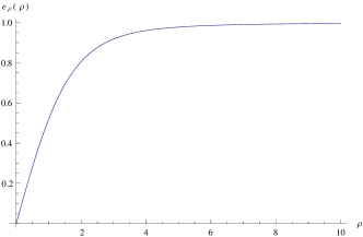
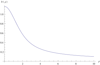
Figure 1: Profile of the radial electric and magnetic fields as funcions of $\rho$: the slope at the origin for $f$ (see eqn.(13)) obtained by our numerical shooting method is $\beta\approx 0.58319$. The electric and magnetic fields in the plots have been rescaled appropriately.

At this point, it is important to stress that the vortex solution for the present model does not exist in the absence of the Chern-Simons term. Indeed, a glimpse at equation (2) shows that the Chern-Simon coupling $k$ induces a charge density proportional to the magnetic field $b$, which turns out to be crucial to source the vortex electric field.

3.1.3 Energy, entropy and free energy:

In the previous section we have shown the existence of vortex solution in the system. A natural question to ask is whether the system will choose it as its ground state or not. In order to answer this question, we write the expression for the energy (6) in the form

$$E_{v} = \frac{\pi|m|^{4}R_{o}^{2}}{\lambda}\int_{a}^{L}\!\!d\rho\rho\left(f^{\prime 2}+\frac{f^{2}}{\rho^{2}}+\frac{1}{2}(f^{2}-1)^{2}\right)\,,$$ (15)

where $a$ is a UV cutoff, and $L$ the size of the system. The vortex is regular at the origin, so we do not expect any singularity in the $a\to 0$ limit. Taking into account the asymptotic behavior (14) one immediately finds that

$$E_{v}\approx E_{core}(R)+\frac{\pi|m|^{4}}{\lambda}\ln\left(\frac{L}{R}\right),$$ (16)

where $E_{core}(R)$ is the finite contribution arising from the energy density integrated up to a distance $R$ bigger than the core radius $R_{o}$.

Since the vortex energy diverges logarithmically with the size of the system, the standard Kosterlitz-Thouless argument follows [11]: energetic considerations imply that at negligible temperatures the system will never choose the vortex configuration, but at finite temperatures, the choice of background is governed by the Helmholtz free energy $F=E-T\,S$ and the entropic contribution could favor vortices for high enough $T$. In our vortex example, this entropic contribution arises from the number of possible places on the plane in which the vortex can sit,

$$S=2k_{B}\ln\left(\frac{L}{a}\right)\,.$$ (17)

The similar logarithmic behavior for both the energy and entropy contributions will compete on the free energy,

$$F = E-TS=$$ (18)

$$= E_{core}(R)+\frac{\pi|m|^{4}}{\lambda}\ln\left(\frac{L}{R}\right)-2k_{B}T\ln\left(\frac{L}{a}\right)\,.$$

As a result, Kosterlitz and Thouless argued that a temperature should exists above which the system lowers its free energy by popping vortex-antivortex pairs out of the anisotropic vacuum [11],[12]. This phenomenon is described in the literature as vortex unbinding and named topological phase transition. The critical temperature $T_{KT}$ for this phase transition can be estimated from the $F=0$ condition, Taking into account the $L$ dependence we find for the present case

$$T_{KT}\approx\frac{\pi|m|^{4}}{2k_{B}\lambda}\,.$$ (19)

Below this critical temperature the system will be in a quasi-long-range ordered anisotropic phase. As soon as the system reaches $T_{KT}$ it will be energetically favored to produce vortices and the quasi-long-range order will be destroyed.

3.2 Hyperbolic plane

Negative curvature spaces have been proposed as interesting setups to cure infrared divergences. The argument is pretty simple [8]: since the volume of space grows exponentially with the distance to the origin, Gauss’ law implies an exponential decay for massless fields. In this section we will analyze the modifications that arise on the vortex solution when we formulate the LCS model on the $2d$-hyperbolic plane[9].

As in the previous section, the vortex solution is easily found when writting the metric in polar coordinates,

$$ds^{2}=R^{2}(d\rho^{2}+\sinh^{2}\!\rho\,d\theta^{2})\,,$$ (20)

here $R$ is the curvature radius of the space. Inserting the static radial ansatz (9) into the equations of motion (5) again with $m^{2}=-|m|^{2}$ leads to

$$f^{\prime\prime}+\frac{1}{\tanh\rho}f^{\prime}-\frac{1}{\tanh^{2}\rho}f-f\left(f^{2}-f_{o}^{2}\right)=0\,,$$ (21)

where $f_{o}^{2}=(R^{2}+\tilde{R}_{o}^{2})/R_{o}^{2}$. The existence of curvature in the $2$-dimensional space results in an equation of motion now depending on a parameter $f_{o}^{2}$ which cannot be re-absorbed.

The behavior for $f$ near the origin coincides with that of flat space (13), but the large distance behavior changes drastically. The relevant case for us is $f_{o}^{2}>1$ which results in a non-zero value at infinity for the electric field and an asymptotic radial profile given by

$$f(\rho)=\sqrt{f_{o}^{2}-1}\left(1-\frac{2}{{f_{o}^{2}-2}}e^{-2\rho}+{\cal O}\left(e^{-4\rho}\right)\right)\,,$$ (22)

Notice that the exponential decay for the profile is independent of the parameters of the model. We have depicted in Fig.(2) the numerical solutions we find for different values of $f_{o}^{2}$.

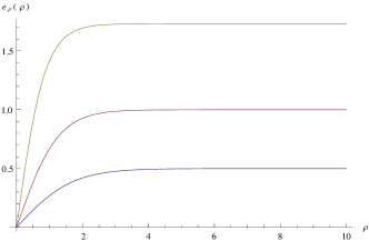
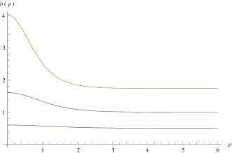
Figure 2: Profile of the electric and magnetic fields in the hyperbolic plane as functions of $\rho$. For $f_{o}^{2}=4,2,1.25$ the corresponding slopes of the electric field at the origin, obtained by our numerical shooting method, are $\beta\approx 2.01093,0.80291,0.30023$ respectively.

The vortex energy functional in the hyperbolic plane case takes the form

$$E_{v}^{{}^{(hyp)}} = \frac{\pi|m|^{4}R_{o}^{4}}{\lambda R^{2}}\int_{a}^{L}d\rho\sinh\rho\left(f^{\prime}\,\!{}^{2}+\frac{f^{2}}{\tanh^{2}\rho}+2\frac{\tilde{R}_{o}^{2}}{R_{o}^{2}}\,\frac{ff^{\prime}}{\tanh\rho}\ +\right.$$ (23)

$$\left.\ \ \ \ \ \ \ \ \ \ \ \ \ \ \ \ \ \ \ \ \ \ \ \ \ \ \ \ \ \ \ \ \ \ \ \ \ \ \ \ \ \ \ \ \ \ \ \ \ +\ \frac{1}{2}{f^{4}}-\frac{R^{2}}{R_{o}^{2}}f^{2}+\tilde{E}_{o}\right),$$

with $a,L$ being respectively UV and IR cutoffs. The energy density behavior near the origin coincides with that of flat space and far away from the origin, although the volume element grows exponentially fast at large distances, the electric field decays more rapidly (see (22)) and overwhelms the divergence. Taking the asymptotic behaviors into account we find that the vortex logarithmic divergence present in flat space is cured by the spatial negative curvature. We have therefore found that the $n=1$ solution is a true soliton (finite energy) for the hyperbolic space case. The appropriate value for $\tilde{E}_{o}$ results

$$\tilde{E}_{o} = \frac{(R^{2}-R_{o}^{2}-\tilde{R}_{o}^{2})(R^{2}-R_{o}^{2}-3\tilde{R}_{o}^{2})}{2m^{4}\tilde{R}_{o}^{4}R_{o}^{4}}\,.$$ (24)

3.3 Sphere

For completeness we will now consider the LCS model formulated on a sphere with metric

$$ds^{2}=R^{2}\left(d\rho^{2}+\sin^{2}\rho\,d\theta^{2}\right)\,,$$ (25)

here $R$ is the radius of the sphere. Introducing the ansatz (9) into (5), the equation of motion with $m^{2}=-|m|^{2}$ results in

$$f^{\prime\prime}+\frac{1}{\tan\rho}f^{\prime}-\frac{1}{\tan^{2}\rho}f-f\left(f^{2}-f_{o}^{2}\right)=0\,,$$ (26)

with $f_{o}^{2}=(R^{2}-\tilde{R}_{o}^{2})/R_{o}^{2}$. To avoid singularities, we should demand the electric field to vanish at the north and south pole of the $2$-sphere. The appropriate boundary conditions in the sphere case result

$$e_{\rho}(\rho,\theta)|_{\rho=0,\pi}=0\Rightarrow f(0)=f(\pi)=0\,.$$ (27)

The asymptotic behavior at the poles coincide with the flat space case and the configurations we obtain with these boundary conditions correspond to a vortex and an antivortex located at antipodes on the 2-sphere. This last fact is a consequence of (2): no net charge can be supported on a compact manifold. Therefore the flux lines emanating from the north pole should end on an equally opposite charge located in our case at the south pole. Some typical profiles are plotted in Fig.(3).

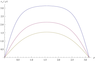
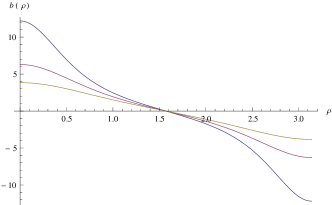
Figure 3: Profile of the electric and magnetic fields for the sphere as function of the azimuthal angle $\rho$ (see eqn.(25)). For $f_{o}^{2}=3,5,10$, the slope of the electric field at the origin are $\beta\approx 1.91747,3.143601,6.090353$.

The energy for the vortex-antivortex configuration on the 2-sphere takes the form

$$E_{v\bar{v}}^{(sph)} = \frac{\pi|m|^{4}R_{o}^{4}}{\lambda R^{2}}\int_{0}^{\pi}d\rho\sin\rho\left(f^{\prime}\,\!{}^{2}+\frac{f^{2}}{\tan^{2}\rho}+\frac{2\tilde{R}_{o}^{2}}{R_{o}^{2}}\frac{ff^{\prime}}{\tan\rho}+\frac{1}{2}{f^{4}}-\frac{R^{2}}{R_{o}^{2}}f^{2}\right)\,,$$ (28)

In the sphere case the energy of the solution is finite due to the compactness of the spatial manifold and the regularity of the solution, there is no need for a compensating constant $E_{o}$.

4 Closing Remarks

We found vortex-like solutions to the Lifshitz-Chern-Simons theory. The presence of the Chern-Simons term is crucial to the existence of such solutions, since it sources the Gauss law (2). The logarithmically divergent energy suggests that a Kostelitz-Thouless transition may occur on the system. To fully clarify the nature of this phase transition a renormalization group analysis along the lines of [13] should be performed, this is currently underway and will be presented elsewhere. Unlike the $U(1)$ global vortex case, extensions to higher winding are non trivial, due to the vector character of the electric field.

Following a suggestion made in [8], we studied vortex solutions of the Lifshitz-Chern-Simons model formulated on the hyperbolic plane. We found, as expected, that the resulting configurations have finite energy. For completeness, we also explore Lifshitz-Chern-Simons vortex solutions on the sphere. In this last case, as in any compact manifold, the solution we found consisted in a vortex-antivortex pair. An open point is to study the stability of such solution.

An important question is whether the flat space version of action (1) at $m=0$ is the most general action describing the critical point. In principle, higher order terms like the introduced in [14] could be added, without breaking the $z=2$ scaling symmetry. We will explore this issue in a separate publication.

References

Appendix A Electromagnetic duality in Lifshitz systems

In this appendix we will shortly review the electromagnetic duality mapping the $k=0$ action (1) into a $z=2$ scalar field theory [1],[17].

We start with the flat space action (1) without the Chern-Simons deformation,

$$S = \int\!dt\,d^{2}\!x\left(e_{i}(\partial_{t}a_{i}-\partial_{i}a_{t})-\frac{1}{2}\left({\kappa^{2}}(\nabla_{i}e_{j})^{2}+b^{2}\phantom{\frac{1}{2}}\!\!\!\!\right)-\frac{1}{2}\left({m^{2}}\,(e_{i})^{2}+\frac{\lambda}{2}(e_{i})^{4}\right)\right).$$

The equations of motion following from the action are

$$(\kappa^{2}\nabla^{2}-m^{2}-\lambda e_{j}^{2})e_{i}=\partial_{i}a_{t}-\partial_{t}a_{i},$$ (30)

$$\partial_{i}e^{i}=0,$$ (31)

$$\epsilon_{ij}\partial_{j}b+\partial_{t}e_{i}=0.$$ (32)

Written in terms of the gauge invariant fields $e_{i},b$ they read

$$(\kappa^{2}\nabla^{2}-m^{2})\epsilon_{ij}\partial_{i}e_{j}-\lambda\epsilon_{ij}\partial_{i}(e_{k}^{2}\,e_{j})=-\partial_{t}b,$$ (33)

$$\partial_{i}e^{i}=0,$$ (34)

$$\epsilon_{ij}\partial_{j}b+\partial_{t}e_{i}=0.$$ (35)

The duality transformation is defined by solving Gauss law (34) as

$$e^{i}=\epsilon^{ij}\partial_{j}\phi.$$ (36)

and then plugging (36) into equation (35). This implies that $b$ can be written in terms of $\phi$ as

$$b=-\partial_{t}\phi.$$ (37)

where a time dependent integration “constant” has been reabsorbed in $\phi$. Replacing (36)-(37) into (33) leads to

$$-(\kappa^{2}\nabla^{2}-m^{2})\nabla^{2}\phi+\lambda\partial_{i}((\nabla\phi)^{2}\partial_{i}\phi)=\partial_{t}^{2}\phi.$$ (38)

This equation of motion for the scalar field can be derived from the action

$$S[\phi]=\int\!dt\,d^{2}\!x\frac{1}{2}\left((\partial_{t}\phi)^{2}-\kappa^{2}(\nabla^{2}\phi)^{2}-m^{2}(\nabla\phi)^{2}-\frac{\lambda}{2}(\nabla\phi)^{4}\right)$$ (39)

The first two terms correspond to the $z=2$ Lifshitz action for a scalar field. As it happens in its electromagnetic dual, the $m^{2}$ term drives the theory away from its $z=2$ fixed point into a $z=1$ IR fixed point. Note that the gauge vector $a_{i},a_{t}$ decouples from $\phi$ and can be integrated out.

In the presence of a CS term, the dualization described above leads to a non-local action for the scalar field [1]. An alternative non-local duality transformation leading to a local equation of motion for the scalar field can be found in [18].

References

- [1] M. Mulligan, C. Nayak and S. Kachru, “An Isotropic to Anisotropic Transition in a Fractional Quantum Hall State,”, Phys. Rev. B 82, 085102 (2010), arXiv:1004.3570 [cond-mat.str-el].
- [2] E. Ardonne, P. Fendley and E. Fradkin, “Topological order and conformal quantum critical points,” Annals Phys. 310 (2004) 493, arXiv:cond-mat/0311466.
- [3] P. Ghaemi, A. Vishwanath, T. Senthil, “Finite temperature properties of quantum Lifshitz transitions between valence bond solid phases: An example of ‘local’ quantum criticality,” Phys. Rev. B 72, 024420 (2005), arXiv:cond-mat/0412409.
- [4] M. Mulligan, C. Nayak, S. Kachru, “Effective Field Theory of Fractional Quantized Hall Nematics,” Phys. Rev. B 84, 195124 (2011), arXiv:1104.0256 [cond-mat.str-el].
- [5] S. C. Zhang, T. H. Hansson, and S. Kivelson, “Effective-Field-Theory Model for the Fractional Quantum Hall Effect,” Phys. Rev. Lett. 62, 82 (1989)
- [6] S. C. Zhang, “The Chern-Simons-Landau-Ginzburg theory of the fractional quantum Hall effect,” Int. J. Mod. Phys. B, (1992)
- [7] Jing Xia, J.P. Eisenstein, L.N. Pfeiffer, and K.W. West, “Evidence for a fractional quantum Hall state with anisotropic longitudinal transport,” arXiv:1109.3219 [cond-mat.str-el].
- [8] C. G. Callan, Jr. and F. Wilczek, “Infrared Behavior At Negative Curvature,” Nucl. Phys. B 340 (1990) 366.
- [9] Local vortices on the hyperbolic plane have appeared in the context of cylindrical instanton solutions in: E. Witten, “Some Exact Multi - Instanton Solutions of Classical Yang-Mills Theory,” Phys. Rev. Lett. 38 (1977) 121.
- [10] A. Vilenkin and E.P.S. Shellard, Cosmic Strings and Other Topological Defects (Cambridge Monographs on Mathematical Physics), Ch. 4, CUP, 2000.
- [11] J. M. Kosterlitz, D. J. Thouless, “Long range order and metastability in two dimensional solids and superfluids,” J. Phys. C 5 (1972) L124.
- [12] J. M. Kosterlitz, D. J. Thouless, “Ordering, metastability and phase transitions in two-dimensional systems,” J. Phys. C C6 (1973) 1181-1203.
- [13] J. V. Jose, L. P. Kadanoff, S. Kirkpatrick and D. R. Nelson, “Renormalization, vortices, and symmetry breaking perturbations on the two-dimensional planar model,” Phys. Rev. B 16, 1217 (1977).
- [14] S. Deser and R. Jackiw, “Higher derivative Chern-Simons extensions,” Phys. Lett. B 451, 73 (1999) arXiv:hep-th/9901125.
- [15] Francois David, “Geometry and field theory of random surfaces and membranes”, included in D. Nelson, T. Piran, S, Weinberg (Eds) “Statistical mechanics of membranes and surfaces”, World Scientific (2004) ISBN 981-238-760-9
- [16] Eduardo Fradkin, David A. Huse, R. Moessner, V. Oganesyan, S. L. Sondhi, On bipartite Rokhsar-Kivelson points and Cantor deconfinement, Phys. Rev. B 69, 224415 (2004), arXiv:cond-mat/0311353.
- [17] A. Vishwanath, L. Balents and T. Senthil, Quantum Criticality and Deconfinement in Phase Transitions Between Valence Bond Solids, Phys. Rev. B69 (2004) 224416.
- [18] S. Deser, R. Jackiw and S. Templeton, “Topologically Massive Gauge Theories,” Annals Phys. 140 (1982) 372 [Erratum-ibid. 185 (1988) 406] [Annals Phys. 185 (1988) 406] [Annals Phys. 281 (2000) 409].