Coexistence of spin-triplet superconductivity with magnetic ordering in an orbitally degenerate system: Hartree-Fock-BCS approximation revisited

Abstract

The Hund’s-rule-exchange induced and coexisting spin-triplet paired and magnetic states are considered within the doubly degenerate Hubbard model with interband hybridization. The Hartree-Fock approximation combined with the Bardeen-Cooper-Schrieffer (BCS) approach is analyzed for the case of square lattice. The calculated phase diagram contains regions of stability of the spin-triplet superconducting phase coexisting with either ferromagnetism or antiferromagnetism, as well as a pure superconducting phase. The influence of the inter-site hybridization on the stability of the considered phases, as well as the temperature dependence of both the magnetic moment and the superconducting gaps, are also discussed. Our approach supplements the well known phase diagrams containing only magnetic phases with the paired triplet states treated on the same footing. We also discuss briefly how to include the spin fluctuations within this model with real space pairing.

I Introduction

The spin-triplet superconducting phase is believed to appear in Sr₂RuO₄ Maeno1994 , UGe₂ Saxena2000 , and URhGe Tateiwa2001 . In the last two compounds the considered type of superconducting phase occurs as coexisting with ferromagnetism. Additionally, even though U atoms in this compounds contain 5f electrons responsible for magnetism, this multiple-band system can be regarded as weakly or moderately correlated electron system, particularly at higher pressure. Originally it has been suggested via a proper quantitative analysis Klejnberg1999 ^-Zegrodnik2011 , that the the intra atomic Hund’s rule exchange can lead in a natural manner to the coexistence of superconductivity with magnetic ordering - ferromagnetism or antiferromagnetism.

The coexisting superconducting and magnetic phases are discussed in this work within an orbitally degenerate two-band Hubbard model using the Hartree-Fock approximation (HF), here combined with the Bardeen-Cooper-Schrieffer (BCS) approach, i.e., in the vicinity of the ferromagnetism disappearance, where also the superconductivity occurs. The particular emphasis is put on the appearance of superconductivity near the Stoner threshold, where the Hartree-Fock-BCS approximation can be regarded as realistic. This type of approach can be formulated also for other systems Puetter2003 .

The alternative suggested mechanism for appearance of superconductivity in those systems is the pairing mediated by ferromagnetic spin fluctuations, which can also appear in the paramagnetic or weakly ferromagnetic phase Anderson . Here, the mean-field approximation provides not only the starting magnetic phase diagram but also a related discussion of the superconducting states treated on equal footing. In this approach the spin-fluctuation contribution appears as a next-order contribution. This is the reason for undertaking a revision of the standard Hartree-Fock approximation. Namely, we concentrate here on the spin triplet states, pure and coexisting with either ferromagnetism or antiferromagnetism, depending on the relative magnitude of microscopic parameters: the Hubbard intra- and inter-orbital interactions, $U$ and $U^{\prime}$, respectively, the Hund’s rule ferromagnetic exchange integral $J$, the relative magnitude of hybridization $\beta_{h}$, and the band filling $n$. The bare band width $W$ is taken as unit of energy. In the concluding Section we discuss briefly, how to outline the approach to include also the quantum fluctuations around this HF-BCS (saddle point) state, as a higher-order contribution.

The role of exchange interactions is crucial in both the so-called t-J model of high temperature superconductivity Spalek1988(2) and in the so-called Kondo-mediated pairing in heavy fermion systems Spalek1988 . In this and the following papers we discuss the idea of real space pairing for the triplet-paired states in the regime of weakly correlated particles and include both the inter-band hybridization and the corresponding Coulomb interactions. We think that this relatively simple approach is relevant to the mentioned at the beginning ferromagnetic superconductors because of the following reasons. Although the effective exchange (Weiss-type) field acts only on the spin degrees of freedom, it is important in determining the second critical field of ferromagnetic superconductor in the so-called Pauli limit Clagton , as the orbital effects in the Cooper-pair breaking process are then negligible. The appearance of a stable coexistent ferromagnetic-superconducting phase means, that either Pauli limiting situation critical field has not been reached in the case of spin-singlet pairing or else, the pairing has the spin-triplet nature, without the component with spin $S^{z}=0$, and then the Pauli limit is not operative.

The present model with local spin-triplet pairing has its precedents of the same type in the case of spin-singlet pairing, i.e., the Hubbard model with $U<0$ Micnas , which played the central role in singling out a nontrivial character of pairing in real space. Here, the same role is being played by the intra-atomic (but inter-orbital) ferromagnetic exchange. We believe that this area of research unexplored so far in detail opens up new possibilities of studies of weakly and moderately correlated magnetic superconductors Nomura2002 .

The structure of this paper is as follows. In Section 2 we define the model and the full Hartee-Fock-BCS approximation (i. e. mean field approximation for magnetic ordering with the concomitant BCS-type decoupling) for the coexistent two-sublattice antiferromagnetic and spin-triplet superconducting phase (cf. also Appendix A for details). For completeness, in Appendix B we include also the analysis of a simpler coexistant superconducting-ferromagnetic phase. In Section 3 we provide a detailed numerical analysis and construct the full phase diagram on the Hund’s rule coupling-band filling plane. We describe also the physical properties of the coexistent phases. In Appendix C we sketch a systematic approach of going beyond Hartree-Fock approximation, i.e., including the spin fluctuations, starting from our Hartree-Fock-BCS state.

II Model and coexistent antiferromagnetic-spin-triplet superconducting phase: mean-field-BCS approximation

We start with the extended orbitally degenerate Hubbard Hamiltonian, which has the form

$$\begin{split}\hat{H}&=\sum_{ij(i\neq j)ll^{\prime}\sigma}t^{ll^{\prime}}_{ij}a_{il\sigma}^{{\dagger}}a_{jl^{\prime}\sigma}+(U^{\prime}+J)\sum_{i}\hat{n}_{i1}\hat{n}_{i2}\\ &+U\sum_{il}\hat{n}_{il\uparrow}\hat{n}_{il\downarrow}-J\sum_{ill^{\prime}(l\neq l^{\prime})}\bigg{(}\mathbf{\hat{S}}_{il}\cdotp\mathbf{\hat{S}}_{il^{\prime}}+\frac{3}{4}\hat{n}_{il}\hat{n}_{il^{\prime}}\bigg{)},\end{split}$$ (1)

where $l=1,2$ label the orbitals and the first term describes electron hopping between atomic sites $i$ and $j$. For $l\neq l^{\prime}$ this term represents electron hopping with change of the orbital (inter-site, inter-orbital hybridization). Next two terms describe the Coulomb interaction between electrons on the same atomic site. However as one can see the second term contains the contribution that originates from the exchange interaction ($J$). The last term expresses the (Hund’s rule) ferromagnetic exchange between electrons localized on the same site, but on different orbitals. This term is regarded as responsible for the local spin-triplet pairing in the subsequent discussion. The components of the spin operator $\mathbf{\hat{S}}_{il}=(\hat{S}^{x}_{il},\hat{S}^{y}_{il},\hat{S}^{z}_{il})$ used in (1) aquire the form

$$\hat{S}^{x,y,z}_{il}=\frac{1}{2}\mathbf{\hat{h}}_{il}^{\dagger}\mathbf{\sigma}_{x,y,z}\mathbf{\hat{h}}_{il},$$ (2)

where $\sigma_{x,y,z}$ are the Pauli matrices and $\mathbf{h}_{il}^{\dagger}\equiv(a^{\dagger}_{il\uparrow},a^{\dagger}_{il\downarrow})$. In our considerations we neglect the interaction-induced intra-atomic singlet-pair hopping ($Ja^{{\dagger}}_{i1\uparrow}a^{{\dagger}}_{i1\downarrow}a_{i2\downarrow}a_{i2\uparrow}+H.c.$) and the correlation induced hopping ($Vn_{1\bar{\sigma}}(a^{\dagger}_{1\bar{\sigma}}a_{2\bar{\sigma}}+a^{\dagger}_{2\bar{\sigma}}a_{1\bar{\sigma}})+1\leftrightarrow 2$ ) Nomura2002 , as they should not introduce any important new qualitative feature in the considered here spin-triplet paired states. What is more important, we assume that $t^{12}_{ij}=t^{21}_{ij}$ and $t^{11}_{ij}=t^{22}_{ij}\equiv t_{ij}$, i.e., the starting degenerate bands have the same width (the extreme degeneracy limit), as we are interested in establishing new qualitative features to the overall phase diagram, that are introduced by the magnetic pairing.

As has already been said, the aim of this work is to examine the spin-triplet superconductivity coexisting with ferromagnetism and antiferromagnetism as well as the pure spin-triplet superconducting phase and the pure magnetically ordered phases. Labels defining the spin-triplet paired phases (A and A1) that are going to be used in this work correspond to those defined for superfluid ³He according to the Refs. Vollhardt and Anderson . Namely in the A phase the superconducting gaps that correspond to Cooper pairs with total spin up and down are equal ($\Delta_{1}=\Delta_{-1}\neq 0$, $\Delta_{0}=0$), whereas in the A1 phase the only nonzero superconducting gap is the one that corresponds to the Cooper pair with total spin up ($\Delta_{1}\neq 0$, $\Delta_{-1}=\Delta_{0}=0$). In this section we show the method of calculations that is appropriate for the superconducting phase coexisting with antiferromagnetism, as well as pure superconducting phase of type A and pure antiferromagnetic phase. The corresponding considerations for the case of ferromagnetically ordered phases and superconducting phase A1 are deferred to the Appendix B.

From the start we make use of the fact that the full exchange term can be represented by the real-space spin-triplet pairing operators, in the following manner

$$J\sum_{ill^{\prime}(l\neq l^{\prime})}\bigg{(}\mathbf{\hat{S}}_{il}\cdotp\mathbf{\hat{S}}_{il^{\prime}}+\frac{3}{4}\hat{n}_{il}\hat{n}_{il^{\prime}}\bigg{)}\equiv 2J\sum_{i,m}\hat{A}^{\dagger}_{im}\hat{A}_{im},$$ (3)

which are of the form

$$\hat{A}^{\dagger}_{i,m}\equiv\left\{\begin{array}[]{cl}a^{\dagger}_{i1\uparrow}a^{\dagger}_{i2\uparrow}&m=1,\\ a^{\dagger}_{i1\downarrow}a^{\dagger}_{i2\downarrow}&m=-1,\\ \frac{1}{\sqrt{2}}(a^{\dagger}_{i1\uparrow}a^{\dagger}_{i2\downarrow}+a^{\dagger}_{i1\downarrow}a^{\dagger}_{i2\uparrow})&m=0.\\ \end{array}\right.$$ (4)

Furthermore the inter-orbital Coulomb repulsion term can be expressed with the use of spin-triplet pairing operators and the spin-singlet pairing operators in the following manner

$$(U^{\prime}+J)\sum_{i}\hat{n}_{i1}\hat{n}_{i2}=(U^{\prime}+J)(\sum_{i}\hat{B}^{\dagger}_{i}\hat{B}_{i}+\sum_{im}\hat{A}^{\dagger}_{im}\hat{A}_{im}),$$ (5)

where

$$\hat{B}^{\dagger}_{i}=\frac{1}{\sqrt{2}}(a^{\dagger}_{i1\uparrow}a^{\dagger}_{i2\downarrow}-a^{\dagger}_{i1\downarrow}a^{\dagger}_{i2\uparrow}),$$ (6)

are the inter-orbital, intra-atomic spin-singlet pairing operators in real space. Using Eq. (3) and (5) one can write down our model Hamiltonian in the form

$$\begin{split}\hat{H}&=\sum_{ij(i\neq j)ll^{\prime}\sigma}t^{ll^{\prime}}_{ij}a_{il\sigma}^{{\dagger}}a_{jl^{\prime}\sigma}+U\sum_{il}\hat{n}_{il\uparrow}\hat{n}_{il\downarrow}\\ &+(U^{\prime}+J)\sum_{i}\hat{B}_{i}^{\dagger}\hat{B}_{i}-(J-U^{\prime})\sum_{im}\hat{A}^{\dagger}_{im}\hat{A}_{im}.\end{split}$$ (7)

It should be noted here that for $J<U^{\prime}$, the inter-orbital Coulomb repulsion suppresses the spin-triplet pairing mechanism and the superconducting phases will not appear in the system in the weak-coupling (Hartree-Fock) limit. For $3d$ electrons Sugano , $U^{\prime}=U-2J$, thus the necessary condition for the pairing to occur in our model is $U<3J$. Usually, for 3d metals we have $U\sim 3J$, so it represents a rather stringent condition for the superconductivity to appear in that situation. We use this relation to fix the parameters for modeling purposes, not limited to 3d systems. This is also because e.g. 5f electrons in uranium compounds lead to a similar behavior as do 3d electrons. One should note that the considered here pairing is based on the intra-atomic inter-orbital ferromagnetic Hund’s rule exchange. A simple extension to the situation with nonlocal J has been considered by X. Dai et al. Puetter2003 . Also, as we consider only weakly correlated regime, where the metallic state is stable, no orbital ordering is expected (cf. Klejnberg and Spałek in Spalek2001 ).

In our considerations the antiferromagnetic state represents the simplest example of the spin-density-wave state. In this state, we can divide our system into two interpenetrating sublattices $A$ and $B$. The average staggered magnetic moment of electrons on each of the $N/2$ sublattice $A$ sites is equal, $<S_{i}^{z}>=<S^{z}_{A}>$, whereas on the remaining $N/2$ sublattice $B$ sites we have $<S_{i}^{z}>=<S^{z}_{B}>\equiv-<S^{z}_{A}>$. In accordance with this division into two sublattices, we define different annihilation operators for each sublattice, namely

$$a_{il\sigma}=\left\{\begin{array}[]{cl}a_{il\sigma A}\quad\textrm{for i}\in A,\\ a_{il\sigma B}\quad\textrm{for i}\in B.\\ \end{array}\right.$$ (8)

The same holds for the creation operators, $a^{\dagger}_{il\sigma}$. We assume that the charge ordering is absent. In this situation, we can write that

$$<S^{z}_{i1A}>=<S^{z}_{i2A}>\equiv\bar{S}^{z}_{s},\quad<S^{z}_{i1B}>=<S^{z}_{i2B}>\equiv-\bar{S}^{z}_{s},$$ (9)

$$<n_{i1A}>=<n_{i2A}>=<n_{i1B}>=<n_{i2B}>\equiv n/2,\quad$$ (10)

where $n$ is the band filling. In what follows, we treat the pairing and the Hubbard parts in the combined mean-field-BCS approximation. In effect, we can write down the Hamiltonian transformed in reciprocal ($\mathbf{k}$) space in the form:

$$\begin{split}\hat{H}_{HF}-\mu\hat{N}&=\sum_{\mathbf{k}l\sigma}\bigg{[}\epsilon_{\mathbf{k}}(a^{\dagger}_{\mathbf{k}l\sigma A}a_{\mathbf{k}l\sigma B}+a^{\dagger}_{\mathbf{k}l\sigma B}a_{\mathbf{k}l\sigma A})-\sigma I\bar{S}^{z}_{s}(\hat{n}_{\mathbf{k}l\sigma A}-\hat{n}_{\mathbf{k}l\sigma B})\bigg{]}\\ &+\sum_{kll^{\prime}(l\neq l^{\prime}\sigma)}\epsilon_{\mathbf{k}12}(a^{\dagger}_{\mathbf{k}l\sigma A}a_{\mathbf{k}l^{\prime}\sigma B}+a^{\dagger}_{\mathbf{k}l\sigma B}a_{\mathbf{k}l^{\prime}\sigma A})+\sum_{\mathbf{k}l\sigma}\bigg{[}\frac{n}{8}(U+2U^{\prime}-J)-\mu\bigg{]}(\hat{n}_{\mathbf{k}l\sigma A}+\hat{n}_{\mathbf{k}l\sigma B})\\ &+\sum_{\mathbf{k},m=\pm 1}(\Delta_{mA}^{*}\hat{A}_{\mathbf{k}mA}+\Delta_{mA}\hat{A}^{\dagger}_{\mathbf{k}mA})+\sum_{\mathbf{k},m=\pm 1}(\Delta_{mB}^{*}\hat{A}_{\mathbf{k}mB}+\Delta_{mB}\hat{A}^{\dagger}_{\mathbf{k}mB})\\ &+\sqrt{2}\sum_{\mathbf{k}}(\Delta_{0A}^{*}\hat{A}_{\mathbf{k}0A}+\Delta_{0A}\hat{A}^{\dagger}_{\mathbf{k}0A})+\sqrt{2}\sum_{\mathbf{k}}(\Delta_{0B}^{*}\hat{A}_{\mathbf{k}0B}+\Delta_{0B}\hat{A}^{\dagger}_{\mathbf{k}0B})-N\frac{n^{2}}{16}(U+2U^{\prime}-J)\\ &+2NI(\bar{S}^{z}_{s})^{2}-\frac{N}{2(J-U^{\prime})}(|\Delta_{1A}|^{2}+|\Delta_{-1A}|^{2}+|\Delta_{1B}|^{2}+|\Delta_{-1B}|^{2}+2|\Delta_{0A}|^{2}+2|\Delta_{0B}|^{2}),\end{split}$$ (11)

where $I\equiv U+J$ is the effective magnetic coupling constant and $\epsilon_{\mathbf{k}1}=\epsilon_{\mathbf{k}2}\equiv\epsilon_{\mathbf{k}}$ is the dispersion relation. The results presented in the next section have been carried out for square lattice with nonzero hopping $t$ between nearest neighbors only. The corresponding bare dispersion relation in a nonhybridized band acquires the form:

$$\epsilon_{\mathbf{k}}=-2t\cos k_{x}-2t\cos k_{y}.$$ (12)

As we are considering the doubly degenerate band model situation, we make a simplifying assumption that the hybridization matrix element $\epsilon_{12\mathbf{k}}=\beta_{h}\epsilon_{\mathbf{k}}$, where $\beta_{h}\in[0,1]$ is the parameter, which specifies the hybridization strength (i.e. represents a second scale of electron energies, in addition to $\epsilon_{\mathbf{k}}$). This means that we have just one active atom per unit cell with a doubly degenerate orbital of the same kind (their spatial asymmetry is disregarded). One should note that the sums in (11) (and in all corresponding equations below) is taken over N/2 independent $\mathbf{k}$ states. In the Hamiltonian written above we have also introduced the superconducting spin-triplet sublattice gap parameters

$$\begin{split}\Delta_{\pm 1A(B)}&\equiv-\frac{2(J-U^{\prime})}{N}\sum_{\mathbf{k}}<\hat{A}_{\mathbf{k},\pm 1A(B)}>,\\ \Delta_{0A(B)}&\equiv-\frac{2(J-U^{\prime})}{\sqrt{2}N}\sum_{\mathbf{k}}<\hat{A}_{\mathbf{k},0A(B)}>.\end{split}$$ (13)

The terms: $N\frac{n^{2}}{16}(U+2U^{\prime}-J)$ and $\frac{n}{8}(U+2U^{\prime}-J)$ in (11 ) can be neglected, as they lead only to a shift of the reference point of the system energy. One should note that since the real-space pairing mechanism is of intra-atomic nature, there is no direct conflict with either ferro- or antiferro-magnetic ordering coexisting with it.

II.1 Antiferromagnetic (Slater) subbands

The diagonalization of the Hamiltonian (11) can be carried out in two steps. In the first step we diagonalize the one particle part of the Hartree-Fock Hamiltonian (the first two sums of (11)). Note that we have to carry out this step first, since we assume the bands are both hybridized and contain pairing part. By introducing the four-composite fermion operator $\mathbf{f}^{\dagger}_{\mathbf{k}\sigma}\equiv(a^{\dagger}_{\mathbf{k}1\sigma A},a^{\dagger}_{\mathbf{k}2\sigma A},a^{\dagger}_{\mathbf{k}1\sigma B},a^{\dagger}_{\mathbf{k}2\sigma B})$, we can express the one particle Hamiltonian in the following form

$$\hat{H}^{0}_{HF}=\sum_{\mathbf{k}\sigma}\mathbf{f}_{\mathbf{k}\sigma}^{\dagger}\mathbf{H}^{0}_{\mathbf{k}\sigma}\mathbf{f}_{\mathbf{k}\sigma},$$ (14)

where $\mathbf{f}_{\mathbf{k}}\equiv(\mathbf{f}^{\dagger}_{\mathbf{k}})^{\dagger}$, and

$$\mathbf{H}^{0}_{\mathbf{k}\sigma}=\left(\begin{array}[]{cccc}-\sigma I\bar{S}^{z}_{s}&0&\epsilon_{\mathbf{k}}&\epsilon_{\mathbf{k}12}\\ 0&-\sigma I\bar{S}^{z}_{s}&\epsilon_{\mathbf{k}12}&\epsilon_{\mathbf{k}}\\ \epsilon_{\mathbf{k}}&\epsilon_{\mathbf{k}12}&\sigma I\bar{S}^{z}_{s}&0\\ \epsilon_{\mathbf{k}12}&\epsilon_{\mathbf{k}}&0&\sigma I\bar{S}^{z}_{s}\end{array}\right).$$ (15)

To diagonalize this Hamiltonian we introduce a generalized Bogoliubov transformation to new operators $\tilde{a}_{kl\sigma A}$ and $\tilde{a}_{kl\sigma B}$ in the following manner

$$\left(\begin{array}[]{cl}a_{\mathbf{k}1\sigma A}\\ a_{\mathbf{k}2\sigma A}\\ a_{\mathbf{k}1\sigma B}\\ a_{\mathbf{k}2\sigma B}\end{array}\right)=\left(\begin{array}[]{cccc}-U^{+}_{\mathbf{k}\sigma}&U^{-}_{\mathbf{k}\sigma}&V^{+}_{\mathbf{k}\sigma}&-V^{-}_{\mathbf{k}\sigma}\\ -U^{+}_{\mathbf{k}\sigma}&-U^{-}_{\mathbf{k}\sigma}&V^{+}_{\mathbf{k}\sigma}&V^{-}_{\mathbf{k}\sigma}\\ V^{+}_{\mathbf{k}\sigma}&-V^{-}_{\mathbf{k}\sigma}&U^{+}_{\mathbf{k}\sigma}&-U^{-}_{\mathbf{k}\sigma}\\ V^{+}_{\mathbf{k}\sigma}&V^{-}_{\mathbf{k}\sigma}&U^{+}_{\mathbf{k}\sigma}&U^{-}_{\mathbf{k}\sigma}\\ \end{array}\right)\left(\begin{array}[]{cl}\tilde{a}_{\mathbf{k}1\sigma A}\\ \tilde{a}_{\mathbf{k}2\sigma A}\\ \tilde{a}_{\mathbf{k}1\sigma B}\\ \tilde{a}_{\mathbf{k}2\sigma B}\end{array}\right),$$ (16)

where

$$\begin{split}U^{(\pm)}_{\mathbf{k}\sigma}=\frac{1}{\sqrt{2}}\bigg{(}1+\frac{\sigma I\hat{S}^{z}_{s}}{\sqrt{(\epsilon_{\mathbf{k}}\pm\epsilon_{\mathbf{k}12})^{2}+(I\bar{S}^{z}_{s})^{2}}}\bigg{)}^{1/2},\\ V^{(\pm)}_{\mathbf{k}\sigma}=\frac{1}{\sqrt{2}}\bigg{(}1-\frac{\sigma I\hat{S}^{z}_{s}}{\sqrt{(\epsilon_{\mathbf{k}}\pm\epsilon_{\mathbf{k}12})^{2}+(I\bar{S}^{z}_{s})^{2}}}\bigg{)}^{1/2}.\end{split}$$ (17)

One should note that the symbols $A$ and $B$ that appear as indexes of the new quasi-particle operators $\tilde{a}_{\mathbf{k}l\sigma A}$ and $\tilde{a}_{\mathbf{k}l\sigma B}$, single out the new, hybridized, quasi-particle sub-bands and do not correspond to the sublattices indices $A$ and $B$ as in the case of operators $a_{\mathbf{k}l\sigma A}$ and $a_{\mathbf{k}l\sigma B}$. The dispersion relations in the new quasi-particle representation acquire the form

$$\begin{split}\tilde{\epsilon}_{\mathbf{k}1A}&=-\sqrt{(\epsilon_{\mathbf{k}}+\epsilon_{\mathbf{k}12})^{2}+(I\bar{S}^{z}_{s})^{2}},\\ \tilde{\epsilon}_{\mathbf{k}1B}&=\sqrt{(\epsilon_{\mathbf{k}}+\epsilon_{\mathbf{k}12})^{2}+(I\bar{S}^{z}_{s})^{2}},\\ \tilde{\epsilon}_{\mathbf{k}2A}&=-\sqrt{(\epsilon_{\mathbf{k}}-\epsilon_{\mathbf{k}12})^{2}+(I\bar{S}^{z}_{s})^{2}},\\ \tilde{\epsilon}_{\mathbf{k}2B}&=\sqrt{(\epsilon_{\mathbf{k}}-\epsilon_{\mathbf{k}12})^{2}+(I\bar{S}^{z}_{s})^{2}}.\end{split}$$ (18)

As one can see, the new dispersion relations do not depend on the spin quantum numbers of the quasi-particle. In general if $\epsilon_{\mathbf{k}12}$ is not $\sim\epsilon_{\mathbf{k}}$, we may have four non-degenerate Slater subbands, which is not the case considered here. To express the pairing operators that are present in the Hamiltonian (11) in terms of the new quasi-particle operators, one can use relations (16) and the definitions (4). The explicit form of the original pairing operators in terms of the newly created quasi-particle operators is provided in Appendix A.

II.2 Quasiparticle states for the coexistent antiferromagnetic and superconducting phase

In the second step of the diagonalization of (11), a generalized Nambu-Bogolubov-De Gennes scheme is introduced to write down the complete H-F Hamiltonian again in the matrix form, which allows for an easy determination of its eigenvalues. With the help of composite creation operator $\mathbf{\tilde{f}}^{\dagger}_{\mathbf{k}\sigma}\equiv(\tilde{a}^{\dagger}_{\mathbf{k}1\sigma A},\tilde{a}_{-\mathbf{k}2\sigma A},\tilde{a}^{\dagger}_{\mathbf{k}1\sigma B},\tilde{a}_{-\mathbf{k}2\sigma B})$, we can construct this new 4x4 Hamiltonian matrix and write

$$\hat{H}_{HF}-\mu\hat{N}=\sum_{\mathbf{k}\sigma}\mathbf{\tilde{f}}_{\mathbf{k}\sigma}^{\dagger}\mathbf{H}_{\mathbf{k}\sigma}\mathbf{\tilde{f}}_{\mathbf{k}\sigma}+2\sum_{\mathbf{k}}(\tilde{\epsilon}_{\mathbf{k}2A}+\tilde{\epsilon}_{\mathbf{k}2B})-2\mu N+C,$$ (19)

with

$$\mathbf{H}_{\mathbf{k}\sigma}\equiv\left(\begin{array}[]{cccc}\tilde{\epsilon}_{\mathbf{k}1A}-\mu&\delta_{1\mathbf{k}\sigma}&0&\delta_{3\mathbf{k}\sigma}\\ \delta_{1\mathbf{k}\sigma}^{*}&-\tilde{\epsilon}_{\mathbf{k}2A}+\mu&\delta_{4\mathbf{k}\sigma}&0\\ 0&\delta_{4\mathbf{k}\sigma}^{*}&\tilde{\epsilon}_{\mathbf{k}1B}-\mu&\delta_{2\mathbf{k}\sigma}\\ \delta_{3\mathbf{k}\sigma}^{*}&0&\delta_{2\mathbf{k}\sigma}^{*}&-\tilde{\epsilon}_{\mathbf{k}2B}+\mu\end{array}\right),$$ (20)

and $\mathbf{\tilde{f}}_{\mathbf{k}}\equiv(\mathbf{\tilde{f}}^{\dagger}_{\mathbf{k}})^{\dagger}$. The parameters $\delta_{l\mathbf{k}\sigma}$ are defined as follows

$$\begin{split}\delta_{1\mathbf{k}\sigma}&=\Delta_{\sigma A}U^{+}_{\mathbf{k}\sigma}U^{-}_{\mathbf{k}\sigma}+\Delta_{\sigma B}V^{+}_{\mathbf{k}\sigma}V^{-}_{\mathbf{k}\sigma},\\ \delta_{2\mathbf{k}\sigma}&=\Delta_{\sigma A}V^{+}_{\mathbf{k}\sigma}V^{-}_{\mathbf{k}\sigma}+\Delta_{\sigma B}U^{-}_{\mathbf{k}\sigma}U^{+}_{\mathbf{k}\sigma},\\ \delta_{3\mathbf{k}\sigma}&=-\Delta_{\sigma A}U^{+}_{\mathbf{k}\sigma}V^{-}_{\mathbf{k}\sigma}+\Delta_{\sigma B}U^{-}_{\mathbf{k}\sigma}V^{+}_{\mathbf{k}\sigma},\\ \delta_{4\mathbf{k}\sigma}&=-\Delta_{\sigma A}V^{+}_{\mathbf{k}\sigma}U^{-}_{\mathbf{k}\sigma}+\Delta_{\sigma B}V^{-}_{\mathbf{k}\sigma}U^{+}_{\mathbf{k}\sigma}.\end{split}$$ (21)

Constant $C$ contains the last two terms of the r. h. s. of expression (11). Hamiltonian (19) and matrix (20) have been written under the assumption that $\Delta_{0A}=\Delta_{0B}\equiv 0$. Calculations for the more general case of nonzero gap parameters for $m=0$ have been also done, but no stable coexisting superconducting and antiferromagnetic solutions have been found numerically. The only coexisting solutions that have been found, fulfill the relation $\Delta_{0A}=\Delta_{0B}\equiv 0$. This fact can be understood by the following argument. As in the antiferromagnetic state all lattice sites have nonzero magnetic moment, the Cooper pairs in the spin-triplet state for $m=0$ (i.e. with the total spin $S^{z}=0$, corresponding $<\hat{A}_{\mathbf{k}0}>$) are not likely to appear. Nevertheless, we present the matrix form of the Hamiltonian (11) for the mentioned most general case, in Appendix A. In our considerations here, we limit also to the situation with the real gap parameters $\Delta_{\pm 1A(B)}^{*}=\Delta_{\pm 1A(B)}$. Then, the straightforward diagonalization of (20) yields to the following Hamiltonian

$$\begin{split}\hat{H}_{HF}-\mu\hat{N}&=\sum_{\mathbf{k}l\sigma}(-1)^{l+1}(\lambda_{\mathbf{k}l\sigma A}\alpha^{\dagger}_{\mathbf{k}l\sigma A}\alpha_{\mathbf{k}l\sigma A}\\ &+\lambda_{\mathbf{k}l\sigma B}\alpha^{\dagger}_{\mathbf{k}l\sigma B}\alpha_{\mathbf{k}l\sigma B})+2\sum_{\mathbf{k}}(\tilde{\epsilon}_{\mathbf{k}2A}+\tilde{\epsilon}_{\mathbf{k}2B})\\ &+\sum_{\mathbf{k}\sigma}(\lambda_{\mathbf{k2\sigma A}}+\lambda_{\mathbf{k2\sigma B}})-2\mu N+C,\end{split}$$ (22)

where $\lambda_{\mathbf{k}l\sigma A(B)}$ are the eigenvalues of the matrix (20) and $\alpha_{\mathbf{k}l\sigma A(B)}$ ($\alpha^{\dagger}_{\mathbf{k}l\sigma A(B)}$) are the quasi-particle annihilation (creation) operators, related to the original annihilation and creation operators $\tilde{a}_{\mathbf{k}l\sigma}$, $\tilde{a}^{\dagger}_{\mathbf{k}l\sigma}$ from the first step of our diagonalization, via generalized Bogoliubov transformation of the form

$$\mathbf{\tilde{f}}_{\mathbf{k}\sigma}=\mathbf{U}^{\dagger}_{\mathbf{k}\sigma}\mathbf{g}_{\mathbf{k}\sigma},$$ (23)

with $\mathbf{g}^{\dagger}_{\mathbf{k}\sigma}\equiv(\alpha^{\dagger}_{\mathbf{k}1\sigma A},\alpha_{-\mathbf{k}2\sigma A},\alpha^{\dagger}_{\mathbf{k}1\sigma B},\alpha_{-\mathbf{k}2\sigma B})$. Eigenvectors of the Hamiltonian matrix (20) are the columns of the diagonalization matrix $\mathbf{U}^{\dagger}_{\mathbf{k}}$. Using the definitions of gap parameters $\Delta_{\pm 1A}$, $\Delta_{\pm 1B}$, the average number of particles per atomic site $n=\sum_{l}<\hat{n}_{il\uparrow A}+\hat{n}_{il\downarrow A}>$, and the average magnetic moment per band per site $\bar{S}^{z}=<\hat{n}_{il\uparrow A}-\hat{n}_{il\downarrow A}>/2$, we can construct the set of self-consistent equations for the mean-field parameters ($\Delta_{\pm 1A}$, $\Delta_{\pm 1B}$, $\bar{S}^{z}$) and for the chemical potential. The averages that appear in the set of self-consistent equations, $<\alpha^{\dagger}_{\mathbf{k}l\sigma A(B)}\alpha_{\mathbf{k}l\sigma A(B)}>$, can be replaced by the corresponding Fermi distribution functions

$$f((-1)^{l+1}\lambda_{\mathbf{k}l\sigma A(B)})=1/[\exp(\beta(-1)^{l+1}\lambda_{\mathbf{k}l\sigma A(B)})+1],$$ (24)

where $\beta=1/k_{B}T$. The eigenvalues and the eigenvectors of (20) are evaluated numerically while executing the numerical procedure of solving the set of self-consistent equations. For a given set of microscopic parameters $n$, $J$, $U$, $U^{\prime}$ and temperature $T$, the set of self-consistent equations has several solutions that correspond to different phases. Free energy can be evaluated for each of the solutions that have been found and the one that corresponds to the lowest value of the free energy is regarded as the stable phase. The expression for the free energy functional in the considered case has the form

$$\begin{split}F&=-\frac{1}{\beta}\sum_{\mathbf{k}l\sigma}\bigg{[}\ln\bigg{(}1+\exp(-\beta(-1)^{l+1}\lambda_{\mathbf{k}l\sigma A})\bigg{)}\\ &+\ln\bigg{(}1+\exp(-\beta(-1)^{l+1}\lambda_{\mathbf{k}l\sigma B})\bigg{)}\bigg{]}\\ &+2\sum_{\mathbf{k}}(\tilde{\epsilon}_{\mathbf{k}2A}+\tilde{\epsilon}_{\mathbf{k}2B})+\sum_{\mathbf{k}\sigma}(\lambda_{\mathbf{k}2\sigma A}\\ &+\lambda_{\mathbf{k}2\sigma B})-\mu(2-n)N+C.\end{split}$$ (25)

Numerical results are carried out for square lattice with nonzero hopping $t$ between the nearest neighbors only.
The described above numerical scheme is executed for the following selection of phases:

• normal state (NS): $\Delta_{\pm 1A(B)}=0$, $\bar{S}^{z}_{s}=0$

• pure superconducting phase type A (A): $\Delta_{\pm 1A(B)}\equiv\Delta\neq 0$, $\bar{S}^{z}_{s}=0$

• pure antiferromagnetic phase (AF): $\Delta_{\pm 1A(B)}=0$, $\bar{S}^{z}_{s}\neq 0$

• coexistent superconducting and antiferromagnetic phase (SC+AF): $\Delta_{\pm 1A(B)}\neq 0$, $\bar{S}^{z}_{s}\neq 0$

The ferromagnetically ordered phases, that will also be included in our considerations in the following Sections, are listed below:

• pure saturated ferromagnetic phase (SFM): $\Delta_{\pm 1A(B)}=0$, $\bar{S}^{z}_{u}=\bar{S}^{z}_{u(max)}\neq 0$

• pure nonsaturated ferromagnetic phase (FM): $\Delta_{\pm 1A(B)}=0$, $0<\bar{S}^{z}_{u}<\bar{S}^{z}_{u(max)}$

• saturated ferromagnetic phase coexistent with superconductivity of type A1 (A1+SFM):
  $\Delta_{1A(B)}\equiv\Delta_{1}\neq 0$, $\Delta_{-1A(B)}=0$, $\bar{S}^{z}_{u}=\bar{S}^{z}_{u(max)}\neq 0$

• nonsaturated ferromagnetic phase coexistent with superconductivity of type A1 (A1+FM):
  $\Delta_{1A(B)}\equiv\Delta_{1}\neq 0$, $\Delta_{-1A(B)}=0$, $0<\bar{S}^{z}_{u}<\bar{S}^{z}_{u(max)}$

It should be noted that $\bar{S}^{z}_{u}$ refers to the uniform magnetic moment per band, per site in the ferromagnetically ordered phases, whereas $\bar{S}^{z}_{s}$ is the staggered magnetic moment that corresponds to the antiferromagnetic phases. One could also consider the so called superconducting phase of type B for which all superconducting gaps (including $\Delta_{0A(B)}$) are equal and different from zero. However this phase never coexists with magnetic ordering. What is more important in the absence of magnetic ordering the superconducting phase A has always lower free energy than the B phase. Therefore the superconducting B phase is absent in the following discussion.

III Results and Discussion

We assume that $U^{\prime}=U-2J$ and $U=2.2J$, so there are actually two independent parameters in the considered model - $n$ and $J$. The energies have been normalized to the bare band-width $W=8|t|$, and $T$ expresses the reduced temperature, $T\equiv k_{B}T/W$.

III.1 Overall phase diagram: coexistent magnetic-paired states

In Fig. 1 a-d we present the complete phase diagrams in coordinates $(n,J)$ for different values of the hybridization parameter $\beta_{h}$. They comprise sizeable regions of stable spin-triplet superconducting phase coexisting with either ferromagnetism or antiferromagnetism, as well as pure superconducting phase A. In the phase SC+AF the calculated gap parameters fulfill the relations

$$\Delta_{+1A}=\Delta_{-1B}\equiv\Delta_{+},$$

$$\Delta_{-1A}=\Delta_{+1B}\equiv\Delta_{-},$$ (26)

$$\Delta_{+}>\Delta_{-}.$$

For the singlet paired state one would have $\Delta_{+1A}=-\Delta_{-1A}$, which is not the case here. For the case of half filled band, $n=2$, the superconducting gaps $\Delta_{+}$ and $\Delta_{-}$ vanish and only pure (Slater type) AF survives. The appearance of the AF state for $n=2$ corresponds to the fact that the bare Fermi-surface topology has a rectangular structure with $Q=(\pi,\pi)$ nesting. This feature survives also for $\beta_{h}\neq 0$. Also, the symmetry of the phase diagrams with respect to half-filled band situation is a manifestation of the particle-hole symmetry, since the bare density of states is symmetric with respect to the middle point of the band.

(a)		(b)
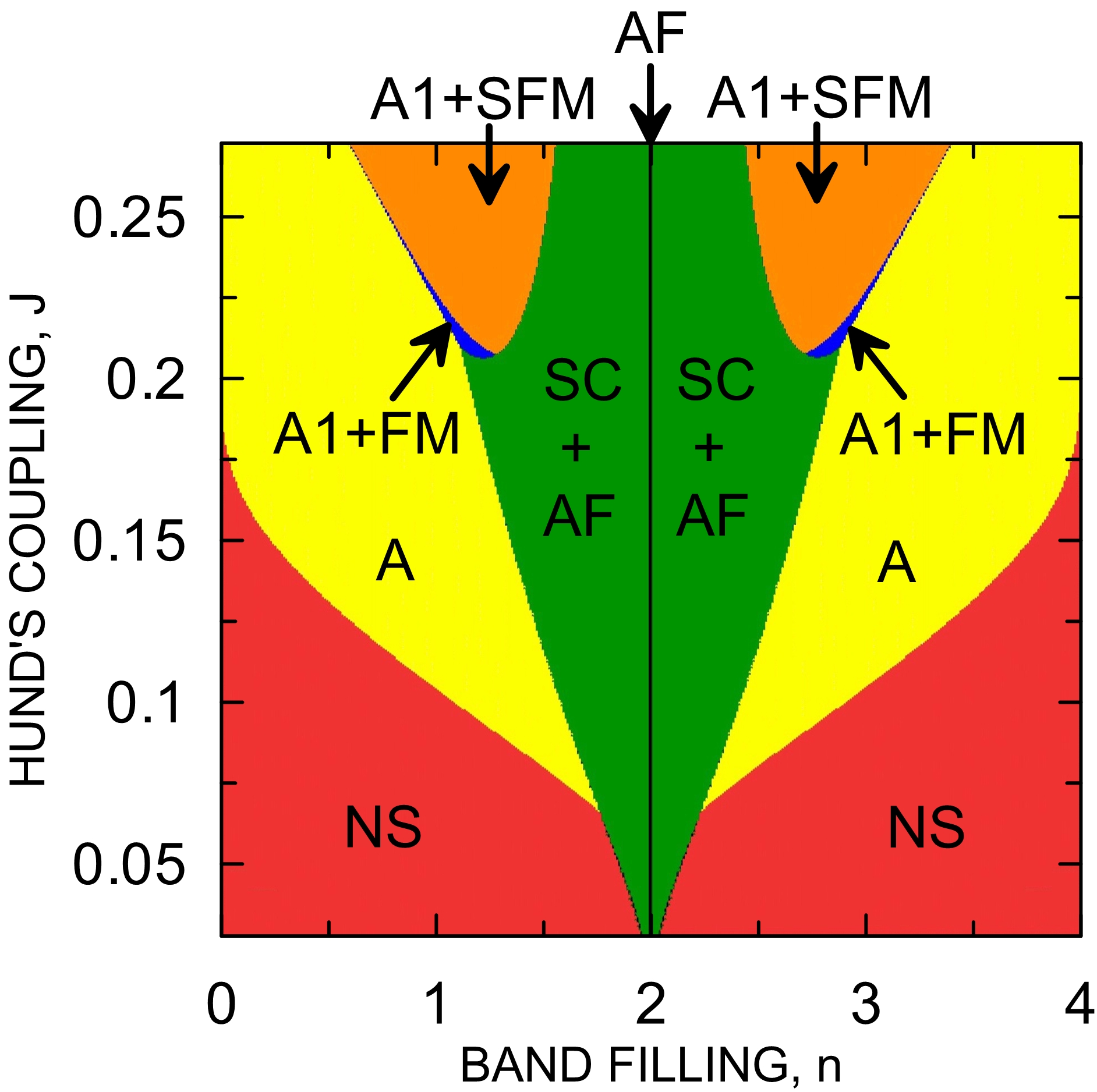
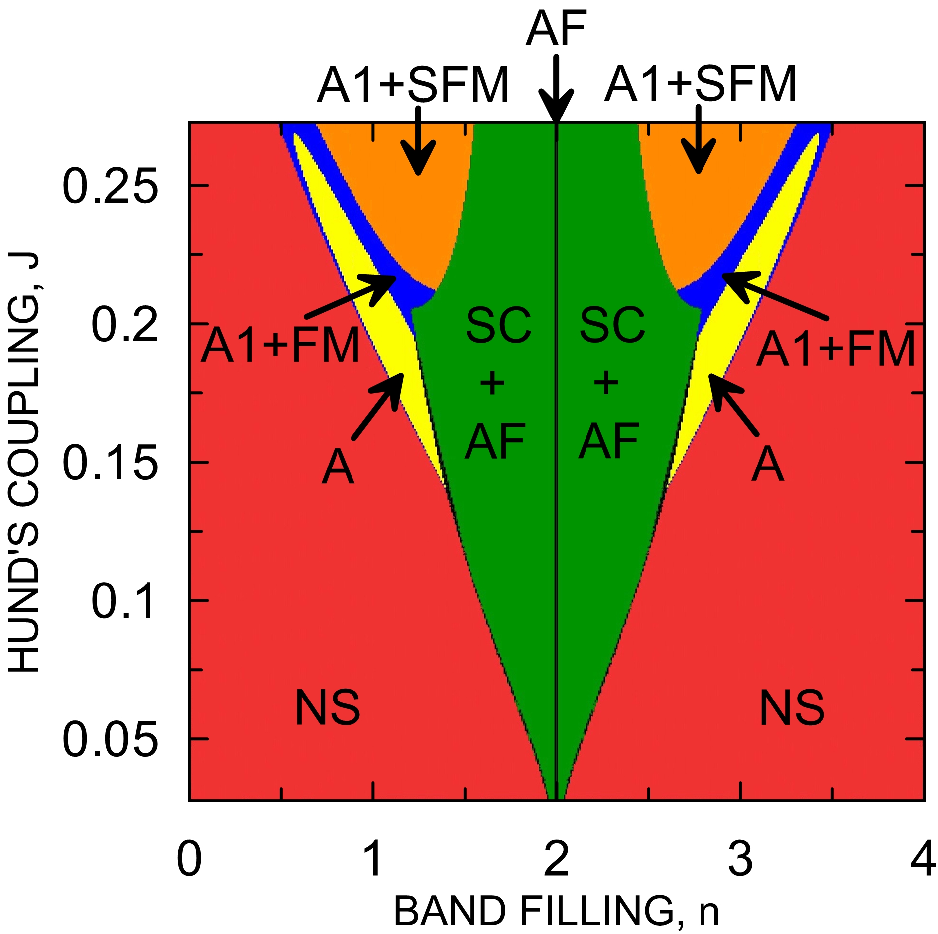
(c)		(d)

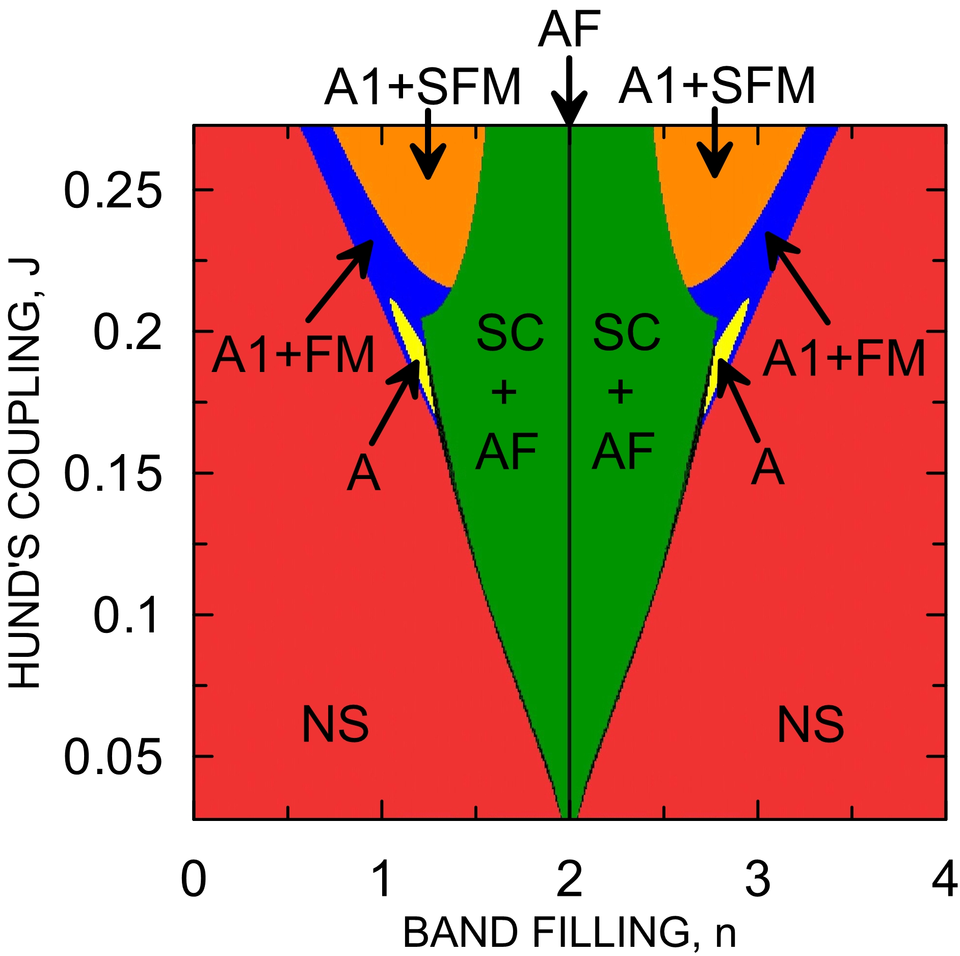
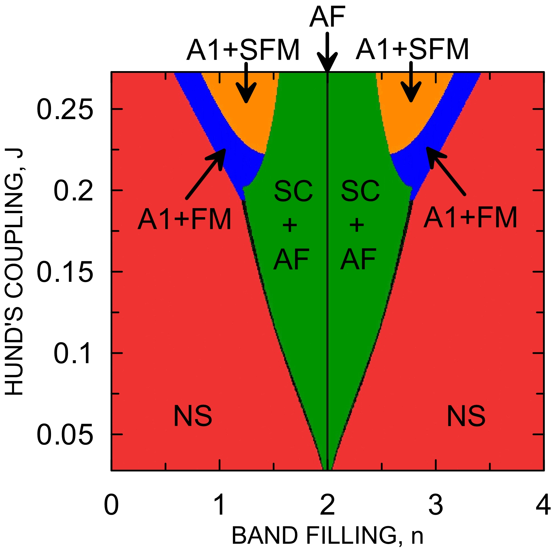
Figure 1: (Color online) Phase diagrams in space $(n,J)$ for $T=10^{-4}$ and for different values of the $\beta_{h}$ parameter: (a) $\beta_{h}=0.00$, (b) $\beta_{h}=0.04$, (c) $\beta_{h}=0.06$, (d) $\beta_{h}=0.11$. Labels representing different phases are described in main text. One sees that practically all magnetic phases here are in fact the coexistent phases with superconductivity except the half filled situation where we have pure AF phase

This feature of the problem provides an additional test for the correctness of the numerical results. It is clearly seen from the presented figures that the influence of hybridization is significant quantitatively when it comes to the superconducting phase A, as the region of its stability narrows down rapidly with the increase of $\beta_{h}$.

The stability areas of A1+FM and NS phases expand on the expense of A and A1+SFM phases. With the further increase of the hybridization, the stability of A phase is completely suppressed, as shown in Fig. 1 d. The regions of stable antiferromagnetically ordered phase do not alter significantly with the increasing hybridization.

(a)
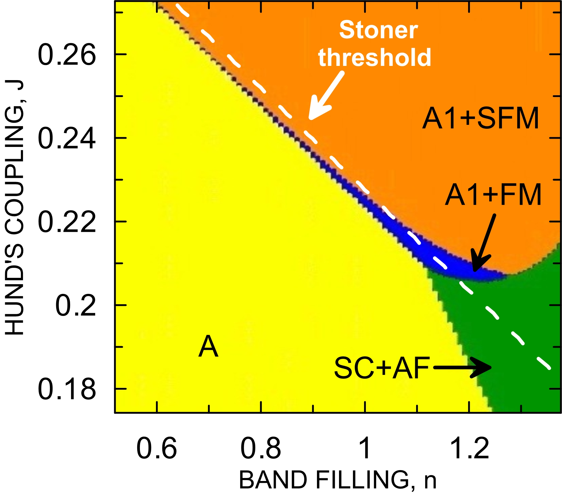
(b)

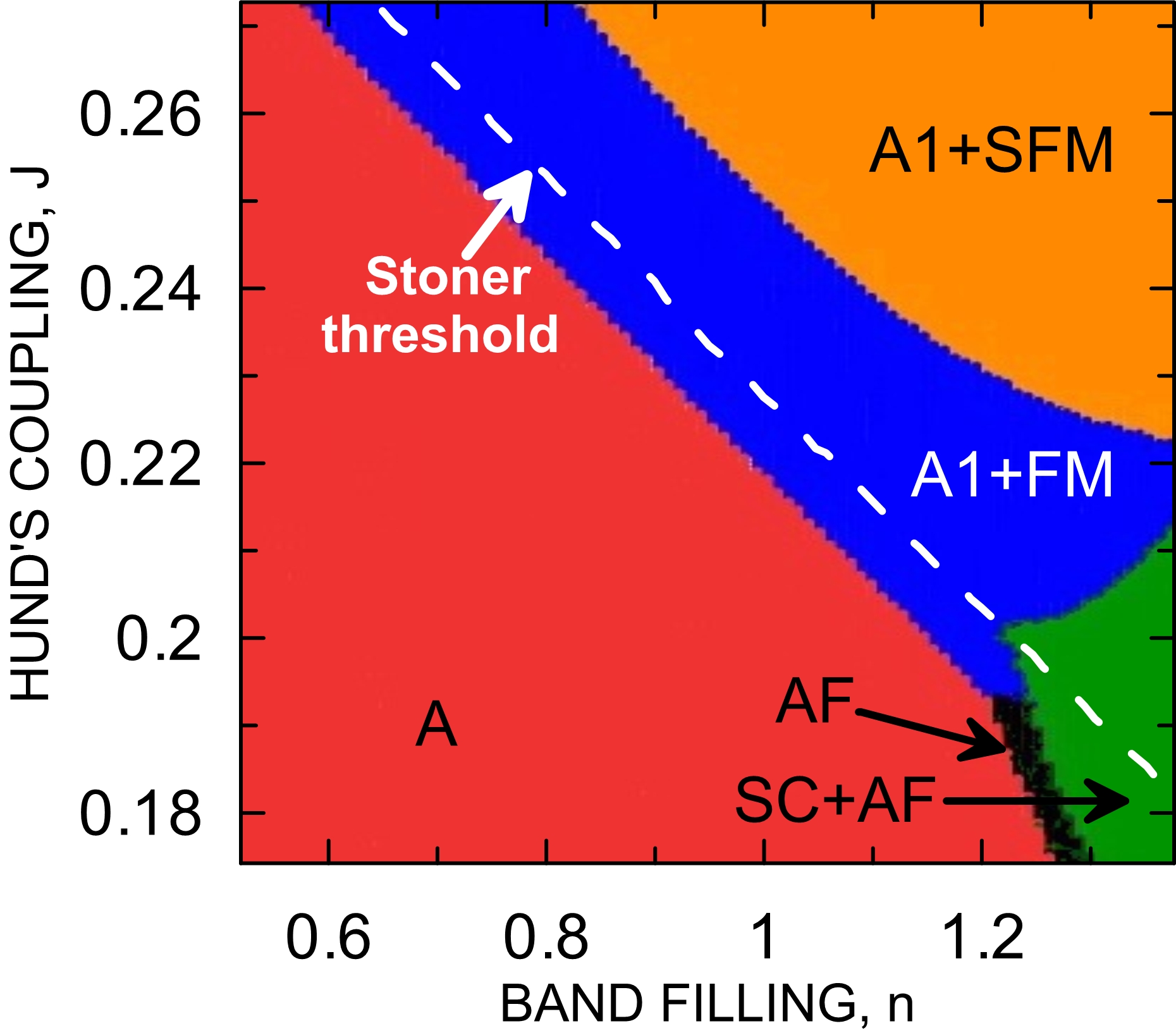
Figure 2: (Color online) Phase diagrams zoomed in space $(n,J)$ with the dashed line marking the Stoner threshold for the onset of pure ferromagnetism. The values of the hybridization parameter are $\beta_{h}$: (a) $\beta_{h}=0.00$, (b) $\beta_{h}=0.11$, while the temperature is $T=10^{-4}$.

To relate the appearance of superconductivity with the onset of ferromagnetism we have marked explicitly in Fig. 2 the Stoner threshold on the phase diagram. One sees clearly that only the A1 phase appearance is related to the onset of ferromagnetism. What is more important, the FM phase coexisting with the paired A1 phase, becomes stable for slightly lower $J$ values than the Stoner threshold for appearance of pure FM phase. The A1+FM coexistence near the Stoner threshold can be analyzed by showing explicitly the magnetization and superconducting gap evolution with increasing $J$. This is shown in Figs. 3 and 4. One sees explicitly that the nonzero magnetization appears slightly below the Stoner threshold and is thus induced by the onset of A1 paired state. In other words, superconductivity enhances magnetism. But opposite is also true, i.e., the gap increases rapidly in this regime, where magnetization changes. The situation is preserved for nonzero hybridization. The transition A$\rightarrow$A1+FM is sharp, as detailed free-energy plot shows. For $\beta_{h}=0.11$ in a certain range of $J$ the superconducting solutions A1+FM and A cannot be found by the numerical procedure. That is why the curves representing the gap parameters $\Delta$ and free energy suddenly break. The most important and surprising conclusion is that in A1+FM phase only the electrons in spin-majority subband are paired. This conclusion may have important practical consequences for spin filtering across NS/A1+FM interface, as discussed at the end. Nevertheless, one should note that the partially polarized (FM) state appears only in a narrow window of $J$ values near the Stoner threshold, at least for the selected density of states.

(a)
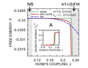
(b)

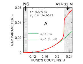
Figure 3: (Color online) Magnetic moment (per orbital per site), ground state energy and superconducting gap as a function of $J$ near the Stoner threshold for $n=1$ and $\beta_{h}=0.0$. Black vertical line in the inset marks the onset of saturated magnetism at the Stoner threshold.

(a)
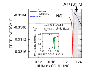
(b)

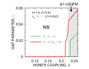
Figure 4: (Color online) Magnetic moment (per orbital per site), ground state energy and superconducting gap as a function of $J$ near the Stoner threshold for $n=1$ and $\beta_{h}=0.11$. Black vertical line in the inset marks the onset of magnetism at the Stoner threshold.

Summarizing, we have supplemented the well known magnetic phase diagrams with the appropriate stable and spin-triplet paired states. A relatively weak hybridization of band states destabilizes pure paired states but stabilizes coexistent superconducting-magnetic phases except for the half-filled band case, when the appearance of the Slater gap at the Fermi level excludes any superconducting state. A very interesting phenomenon of pairing for one-spin (majority) electrons occurs near the Stoner threshold for the onset of FM phase and extends to the regime slightly below threshold.

III.2 Detailed physical properties

In Figs. 5 and 6 we show the low-temperature values of superconducting gaps and the staggered magnetic moment as a function of band filling. In the SC+AF phase both gap parameters $\Delta_{+}$ and $\Delta_{-}$ decrease continuously to zero as the system approaches the half filling. On the contrary, the staggered magnetic moment $\bar{S}^{z}_{s}$ reaches then the maximum. For the case of $\beta_{h}=0.0$, below the critical value of band filling, $n_{c}\approx 1.45$ , the gap parameters $\Delta_{+}$ and $\Delta_{-}$ are equal and the staggered magnetic moment vanishes. In this regime the superconducting phase of type A is the stable one. For A phase the superconducting gap decreases with the band-filling decrease and becomes zero for some particular value of $n$. Below that value the NS (paramagnetic state) is stable. It is clearly seen that the appearance of two gap parameters above $n_{c}$ is connected with the onset of the staggered-moment structure, as above $n_{c}$ we have $S_{s}^{z}\neq 0$ (cf. Fig. 5b). For comparison, we also show the staggered moment for pure AF in Figs. 5b and 6b (dashed line). As one can see, the appearance of SC increases slightly the staggered moment in SC+AF phase. For $\beta_{h}=0.11$ below some critical value of band filling $n_{c}\approx 1.473$ in a very narrow range of $n$, a pure AF phase is stable. The inset in Fig. 6a shows that there is aweak first-order transition between the AF+SC and SC phases as a function of doping. The A phase is not stable in this case.

(a)
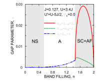
(b)

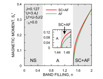
Figure 5: (Color online) Low temperature values of the superconducting gaps and the staggered magnetic moment both as a function of band filling for $\beta_{h}=0$ and $J=0.175$. The stable phases are appropriately labelled in the regimes of their stability. Note that $\Delta_{-}<<\Delta_{+}$, i.e., the paired state is closer to A1 state than to A state in the coexistent regime.

(a)
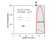
(b)

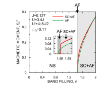
Figure 6: (Color online) Low temperature values of the superconducting gaps and the staggered magnetic moment as a function of band filling for $\beta_{h}=0.11$ and $J=0.175$. Note the disappearance of the pure A phase and that again $\Delta_{-}<<\Delta_{+}$. The inset in (b) illustrates the fact that, a pure AF phase appears in a very narrow regime of $n$ before the SC+AF phase becomes stable, whereas the inset in (a) shows the free energy of those two phases for $n$ close to $n_{C}$ when a weak first-order transition occurs.

One should mention that the easiness, with which the superconducting triplet state is accommodated within the antiferromagnetic phase stems from the fact that the SC gaps have an intra-atomic origin and the corresponding spins have then the tendency to be parallel. Therefore, the pairs respect the Hund’s rule and do not disturb largely the staggered-moment structure, which is of interatomic character.

In Fig. 7 we show temperature dependence of the free energy for the six considered phases, for the set of microscopic parameters selected to make the SC+AF phase stable at $T=0$ and for $\beta_{h}=0$. Because the free-energy values of the A and NS phases are very close, we exhibit their temperature dependences zoomed in Fig. 7b. The same is done for the free energy of phases A1+FM and FM. For the same values of $n$, $J$, $U$ and $U^{\prime}$, the temperature dependence of the superconducting gaps and the staggered magnetic moment in SC+AF phase are shown in Fig. 8, for selected $\beta_{h}$ values. For given $\beta_{h}$ below the superconducting critical temperature $T_{S}$, the staggered magnetic moment and the superconducting gaps have all nonzero values which means, that we are dealing with the coexistence of superconductivity and antiferromagnetism in this range of temperatures. Both $\Delta_{+}$ and $\Delta_{-}$ vanish at $T_{S}$, while the staggered magnetic moment vanishes at the Néel temperature, $T_{N}>>T_{S}$. In Fig. 9 one can observe that there are two typical mean-field discontinuities in the specific-heat at $T_{S}$ and $T_{N}$ for a given $\beta_{h}$. The first of them, at $T_{S}$, corresponds to the phase transition from the SC+AF phase to the pure AF phase, while the second, at $T_{N}$, corresponds to the transition from the AF phase to the NS phase. The values of the ratios of the specific heat jump ($\Delta c/c_{N}$) at $T_{C}$ that correspond to $\beta_{h}=0.0$, $0.4$, $0.6$, are 15.075, 16.298, 17.375 respectively. No antiferromagnetic gap is created, since we have number of electrons $n<2$. The specific heat discontinuity at AF transition is due to the change of spin entropy near $T_{N}$. For $n=2$ the formation of the Slater gap at $T_{N}$ makes the superconducting transition to disappear. As one can see form Figs. 8 and 9, with the increase of $\beta_{h}$ the critical temperature $T_{S}$ is decreasing slightly while the Néel temperature increases, but the ratio remains almost fixed, $T_{N}/T_{C}\approx 10$.

(a)
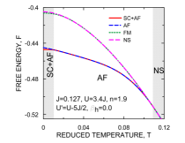
(b)

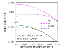
Figure 7: Color online) (a) Temperature dependence of the free energy for considered phases, for $n=1.9$ and $J=0.175$ when the SC+AF phase is stable at $T=0$. The free-energy values of A and NS phases are very close, so we exhibit their temperature dependence blown up in part (b).

(a)
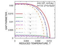
(b)

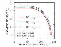
Figure 8: (Color online) Temperature dependences of the superconducting gaps $\Delta_{+}$, $\Delta_{-}$ and of the staggered magnetic moment for $n=1.9$, $J=0.175$ and for selected values of the $\beta_{h}$ parameter. Note that $T_{S}<<T_{N}$.

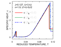
Figure 9: (Color online) Temperature dependence of the specific heat for $n=1.9$, $J=0.175$ and for selected values of $\beta_{h}$ parameter. The behavior is almost independent of $\beta_{h}$ value and the ratio $T_{N}/T_{S}\approx 10$.

Temperature dependence of free energies of relevant phases are presented in Fig. 10 ($\beta_{h}=0$) for the microscopic parameters selected to make the A1+FM phase stable at $T=0$. Free energies for A and A1+FM phases are drawn only in the low-$T$ regime (Fig. 10b) for the sake of clarity. The corresponding temperature dependence of the superconducting gaps, magnetic moment, and specific heat in A1+FM phase for three selected values of $\beta_{h}$ are shown in Fig. 11. Analogously as in the SC+AF case, the system undergoes two phase transitions. The influence of hybridization on the temperature dependences is also similar to that in the case of coexistence of superconductivity with antiferromagnetism. With the increasing $\beta_{h}$, the critical temperature-$T_{S}$ is decreasing slightly, whereas the Curie temperature, $T_{C}$ is slightly increasing, but still $T_{C}/T_{S}\approx 5$. The values of the ratios of the specific heat jump ($\Delta c/c_{N}$) at $T_{C}$ that correspond to $\beta_{h}=0.0$, $0.2$, $0.4$, are 1.329, 1.421, 0.793 respectively.

For the sake of completeness, in Fig. 12 we provide the temperature dependence of superconducting gap for the values of parameters that correspond to stable pure superconducting phase of type A at $T=0$ and for three different values of $\beta_{h}$. In this case, neither the antiferromagnetically ordered nor the pure ferromagnetic phases do exist. As in previous cases, the increasing hybridization decreases $T_{S}$. It should be noted that the values of $\beta_{h}$ are very close to zero. This is necessary to assume for the A phase to appear. The values of the ratios of the specific heat jump ($\Delta c/c_{N}$) at $T_{C}$ that correspond to $\beta_{h}=0.0$, $0.035$, $0.006$, are 1.382, 1.326, 1.202 respectively.

In Table 1 we have assembled the exemplary values of mean field parameters, chemical potential, as well as free energy for two different sets of values of microscopic parameters corresponding to the low-temperature stability of two considered here superconducting phases: SC+AF and A1+FM. For the two sets of values of $n$ and $J$, the free energy difference between the stable and first unstable phases is of order $10^{-3}$. The values for the stable phases are underlined.

(a)
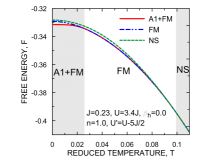
(b)

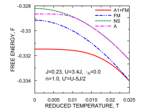
Figure 10: (Color online) Temperature dependence of the free energy for $n=1.0$ and $J=0.31625$ when the A1+FM phase is stable at $T=0$. AF phases does not appear in this case. Free energies for A and A1+FM phases are shown in the low-$T$ regime (b) for the sake of clarity.

(a)
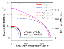
(b)

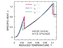
Figure 11: (Color online) Temperature dependence of the superconducting gaps $\Delta_{+}$, $\Delta_{-}$, magnetic moment (a), and specific heat (b), for $n=1.0$, $J=0.31625$ and for selected values of $\beta_{h}$. Qualitative features do not alter appreciably even for $\beta_{h}=0.4$. The ratio $T_{C}/T_{S}\approx 5$.

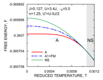
Figure 12: (Color online) Temperature dependences of the superconducting gaps $\Delta_{+}$, $\Delta_{-}$ (a), and the specific heat (b) for $n=1.25$, $J=0.175$ and for selected values of $\beta_{h}$ parameter.

Table 1: Exemplary values of the mean field parameters, the chemical potential, and the free energy of the considered phases at $T=10^{-4}$, for two different sets of values of microscopic parameters: $n$, $J$. The underlined values correspond the stable phases. The numerical accuracy is better than the last digit.

		$n=1.9$	$n=1.0$
parameter	phase	$J=0.175$	$J=0.31625$
$\Delta$	A	0.0097911	0.0208481
$\Delta$	A1+FM	0.0056821	0.0482677
$\Delta_{+}$	SC+AF	0.0210081	-
$\Delta_{-}$	SC+AF	0.0017366	-
$S^{z}_{u}$	A1+(S)FM	0.1134254	0.2500000
$S^{z}_{u}$	(S)FM	0.1144301	0.2500000
$S^{z}_{s}$	SC+AF	0.3340563	-
$S^{z}_{s}$	AF	0.3314687	-
$\mu$	A	-0.0107669	-0.1815757
$\mu$	NS	-0.0094009	-0.1799612
$\mu$	A1+(S)FM	-0.0175982	-0.2530000
$\mu$	(S)FM	-0.0178066	-0.253000
$\mu$	SC+AF	-0.1708890	-
$\mu$	AF	-0.1859011	-
$F$	A	-0.4050464	-0.3286443
$F$	NS	-0.4048522	-0.3282064
$F$	A1+(S)FM	-0.4062039	-0.3314652
$F$	(S)FM	-0.4061793	-0.3291425
$F$	SC+AF	-0.4489338	-
$F$	AF	-0.4469097	-

IV Conclusions and Outlook

We have carried out the Hartree-Fock-BCS analysis of the hybridized two-band Hubbard model with the Hund’s-rule induced magnetism and spin-triplet pairing. We have determined the regions of stability of the spin-triplet paired phases with $\Delta_{0}\equiv 0$, coexisting with either ferromagnetism (A1+FM) or antiferromagnetism (SC+AF), as well as pure paired phase (A). We have analyzed in detail the effect of inter band hybridization on stability of the those phases. The hybridization reduces significantly the stability regime of the superconducting phase A, mainly in favor of the paramagnetic (normal) phase, NS. For large enough value of $\beta_{h}$ ($\beta_{h}>0.08$), the A phase disappears altogether. When it comes to magnetism, with the increase of $\beta_{h}$, the stability regime of the saturated ferromagnetically ordered phase is reduced in favor of the non-saturated. The influence of the hybridization on the low-temperature stability of the SC+AF phase is not significant. When the system is close to the half filling, the SC+AF phase is the stable one. However, for the half filled band case ($n=2$), the superconductivity disappears and only pure antiferromagnetic state survives, since the nesting effect of the two-dimentional band structure prevails then.

We have also examined the temperature dependence of the order parameters and the specific heat. For both coexistent superconducting and magnetically ordered phases (SC+AF and A1+FM) one observes two separate phase transitions with the increasing temperature. The first of them, at substantially lower temperature ($T_{S}$), is the transition from the superconducting-magnetic coexistent phase to the pure magnetic phase and the second, occuring at much higher temperature ($T_{N}$ or $T_{C}$), is from the magnetic to the paramagnetic phase (NS). The hybridization has a negative influence on the spin-triplet superconductivity, since it reduces the critical temperature for each type of the spin-triplet superconducting phase considered here. On the other hand, the Curie ($T_{C}$) and the Néel ($T_{N}$) temperatures are increasing with the increase of the $\beta_{h}$ parameter, as it generally increases the density of states at the Fermi level (for appropriate band fillings).

One sholud note that since the pairing is intra-atomic in nature the spin-triplet gaps $\Delta_{m}$ are of the $s$ type. This constitutes one of the differences with the corresponding situation for superfluid ${}^{3}He$, where they are of $p$ type Anderson .

It is also important to note that the paired state appears both below and above the Stoner threshold for the onset of ferromagnetism (cf. Fig. 2), though its nature changes (A and A1 states, respectively). In the ferromagnetically ordered phase only the spin-majority carriers are paired. This is not the case for AF+SC phase. It would be very interesting to try to detect such highly unconventional SC phase. In particular the Andreev reflection and in general, the NS/SC conductance spectroscopy will have an unusual character. We should see progress along this line of research soon.

As mentioned before all the results presented in the previous section has been obtained assuming that $U=2.2J$ and $U^{\prime}=U-2J$. Having said that the value of $J^{H}=J-U^{\prime}$ determines the strength of the pairing mechanism while $I=U+J$ is the effective magnetic coupling constant, one can roughly predict how will the change in the relations between $U$, $U^{\prime}$, and $J$ result. It seems reasonable to say that the larger is $J$ with respect to $U^{\prime}$ the stronger the superconducting gap in the paired phases. This would also result in the increase of $T_{C}$ and a corresponding enlargement of the area occupied by the superconducting phases on the diagrams. Furthermore the increase of $U$ with respect to $J$ should result in the increase of the ratios $T_{C}/T_{S}$ and $T_{N}/T_{S}$. This is because in that manner we make the magnetic coupling stronger with respect to the pairing. If we however increase $U$ but do not change $J^{H}$, then the strength of the pairing would be the same but the magnetic coupling constant would be stronger so this would favor the coexistent magnetic and superconducting phases with respect to the pure superconducting phase. Quite stringent necessary condition for the pairing to appear $J>U^{\prime}$ (equivalent to $3J>U$ if we assume $U^{\prime}=U-2J$, as has been done here) indicates that only in specific materials one would expect for the Hund’s rule to create the superconducting phase. This may explain why only in very few compounds the coexistent ferromagnetic and superconducting phase has been indeed observed. Obviously, one still has to add the paramagnon pairing (cf. Appendix C).

It should be noted that more exotic magnetic phases may appear in the two-band model Inagaki1973 . Here, we neglect those phases because of two reasons. First the lattice selected for analysis is bipartite, with strong nesting (AF tendency). Second the additional ferrimagnetic, spiral, etc., phase might appear if we assumed that the second hopping integral $t^{\prime}\neq 0$. Inclusion of $t^{\prime}$ would require a separate analysis, as the lattice becomes frustrated then.

V Acknowledgments

M.Z. has been partly supported by the EU Human Capital Operation Program, Polish Project No. POKL.04.0101-00-434/08-00. J.S. acknowledges the financial support from the Foundation for Polish Science (FNP) within project TEAM and also, the support from the Ministry of Science and Higher Education, through Grant No. N N 202 128 736.

Appendix A. Hamiltonian matrix form in the coexistent SC+AF phase and quasiparticle operators

In this Appendix we show the general form of the Hamiltonian matrix $\mathbf{H}_{\mathbf{k}}$ and the pairing operators expressed in terms of the quasi-particle creation operators from the first step of the diagonalization procedure disscused in section 2.

For the case of nonzero gap parameters $\Delta_{0A(B)}$ we have to use eight element composite creation operator

$$\begin{split}\mathbf{\tilde{f}}^{\dagger}_{\mathbf{k}}\equiv(\tilde{a}^{\dagger}_{\mathbf{k}1\uparrow A},\tilde{a}^{\dagger}_{\mathbf{k}1\downarrow A},\tilde{a}_{-\mathbf{k}2\uparrow A},\tilde{a}_{-\mathbf{k}2\downarrow A},\tilde{a}^{\dagger}_{\mathbf{k}1\uparrow B},\\ \tilde{a}^{\dagger}_{\mathbf{k}1\downarrow B},\tilde{a}_{-\mathbf{k}2\uparrow B},\tilde{a}_{-\mathbf{k}2\downarrow B}),\end{split}$$

to write down the Hamiltonian (11) in the matrix form

$$\hat{H}_{HF}-\mu\hat{N}=\sum_{\mathbf{k}}\mathbf{\tilde{f}}_{\mathbf{k}}^{\dagger}\mathbf{H}_{\mathbf{k}}\mathbf{\tilde{f}}_{\mathbf{k}}+2\sum_{\mathbf{k}}(\tilde{\epsilon}_{\mathbf{k}2A}+\tilde{\epsilon}_{\mathbf{k}2B})-2\mu N+C,$$ (27)

where $\mathbf{\tilde{f}}_{\mathbf{k}}\equiv(\mathbf{\tilde{f}}^{\dagger}_{\mathbf{k}})^{\dagger}$ , and

$$\mathbf{H}_{\mathbf{k}}=\left(\begin{array}[]{cccccccc}\tilde{\epsilon}_{\mathbf{k}1A}-\mu&0&\delta_{1\mathbf{k}\uparrow\uparrow}&\delta_{1\mathbf{k}\uparrow\downarrow}&0&0&\delta_{3\mathbf{k}\uparrow\uparrow}&\delta_{3\mathbf{k}\uparrow\downarrow}\\ 0&\tilde{\epsilon}_{\mathbf{k}1A}-\mu&\delta_{1\mathbf{k}\downarrow\uparrow}&\delta_{1\mathbf{k}\downarrow\downarrow}&0&0&\delta_{3\mathbf{k}\downarrow\uparrow}&\delta_{3\mathbf{k}\downarrow\downarrow}\\ \delta^{*}_{1\mathbf{k}\uparrow\uparrow}&\delta^{*}_{1\mathbf{k}\downarrow\uparrow}&-\tilde{\epsilon}_{\mathbf{k}2A}+\mu&0&\delta_{4\mathbf{k}\uparrow\uparrow}&\delta_{4\mathbf{k}\downarrow\uparrow}&0&0\\ \delta^{*}_{1\mathbf{k}\uparrow\downarrow}&\delta^{*}_{1\mathbf{k}\downarrow\downarrow}&0&-\tilde{\epsilon}_{\mathbf{k}2A}+\mu&\delta_{4\mathbf{k}\uparrow\downarrow}&\delta_{4\mathbf{k}\downarrow\downarrow}&0&0\\ 0&0&\delta^{*}_{4\mathbf{k}\uparrow\uparrow}&\delta^{*}_{4\mathbf{k}\uparrow\downarrow}&\tilde{\epsilon}_{\mathbf{k}1B}-\mu&0&\delta_{2\mathbf{k}\uparrow\uparrow}&\delta_{2\mathbf{k}\uparrow\downarrow}\\ 0&0&\delta^{*}_{4\mathbf{k}\downarrow\uparrow}&\delta^{*}_{4\mathbf{k}\downarrow\downarrow}&0&\tilde{\epsilon}_{\mathbf{k}1B}-\mu&\delta_{2\mathbf{k}\downarrow\uparrow}&\delta_{2\mathbf{k}\downarrow\downarrow}\\ \delta^{*}_{3\mathbf{k}\uparrow\uparrow}&\delta^{*}_{3\mathbf{k}\downarrow\uparrow}&0&0&\delta^{*}_{2\mathbf{k}\uparrow\uparrow}&\delta^{*}_{2\mathbf{k}\downarrow\uparrow}&-\tilde{\epsilon}_{\mathbf{k}2B}+\mu&0\\ \delta^{*}_{3\mathbf{k}\uparrow\downarrow}&\delta^{*}_{3\mathbf{k}\downarrow\downarrow}&0&0&\delta^{*}_{2\mathbf{k}\uparrow\downarrow}&\delta^{*}_{2\mathbf{k}\downarrow\downarrow}&0&-\tilde{\epsilon}_{\mathbf{k}2B}+\mu\\ \end{array}\right).$$ (28)

The $\delta_{l\mathbf{k}\sigma\sigma^{\prime}}$ are the generalization of parameters introduced earlier in Eq. (16).

$$\begin{split}\delta_{1\mathbf{k}\sigma\sigma^{\prime}}&=\Delta_{\sigma\sigma^{\prime}A}U^{+}_{\mathbf{k}\sigma}U^{-}_{\mathbf{k}\sigma^{\prime}}+\Delta_{\sigma\sigma^{\prime}B}V^{+}_{\mathbf{k}\sigma}V^{-}_{\mathbf{k}\sigma^{\prime}},\\ \delta_{2\mathbf{k}\sigma\sigma^{\prime}}&=\Delta_{\sigma\sigma^{\prime}A}V^{+}_{\mathbf{k}\sigma}V^{-}_{\mathbf{k}\sigma^{\prime}}+\Delta_{\sigma\sigma^{\prime}B}U^{+}_{\mathbf{k}\sigma}U^{-}_{\mathbf{k}\sigma^{\prime}},\\ \delta_{3\mathbf{k}\sigma\sigma^{\prime}}&=-\Delta_{\sigma\sigma^{\prime}A}U^{+}_{\mathbf{k}\sigma}V^{-}_{\mathbf{k}\sigma^{\prime}}+\Delta_{\sigma\sigma^{\prime}B}V^{+}_{\mathbf{k}\sigma}U^{-}_{\mathbf{k}\sigma^{\prime}},\\ \delta_{4\mathbf{k}\sigma\sigma^{\prime}}&=-\Delta_{\sigma\sigma^{\prime}A}V^{+}_{\mathbf{k}\sigma}U^{-}_{\mathbf{k}\sigma^{\prime}}+\Delta_{\sigma\sigma^{\prime}B}U^{+}_{\mathbf{k}\sigma}V^{-}_{\mathbf{k}\sigma^{\prime}},\end{split}$$ (29)

where $\Delta_{\uparrow\uparrow A(B)}=\Delta_{+1A(B)}$, $\Delta_{\downarrow\downarrow A(B)}=\Delta_{-1A(B)}$, $\Delta_{\downarrow\uparrow A(B)}=\Delta_{\uparrow\downarrow A(B)}=\Delta_{0A(B)}$.

Below we present the pairing operators expressed in terms of the quasi-particle creation operators that we have introduced during the first step of the diagonalization procedure of the Hamiltonian (11).

$$\begin{split}\hat{A}^{\dagger}_{\mathbf{k}\sigma A}&=U^{+}_{\mathbf{k}\sigma}U^{-}_{\mathbf{k}\sigma}\tilde{a}^{\dagger}_{\mathbf{k}1\sigma A}\tilde{a}^{\dagger}_{-\mathbf{k}2\sigma A}+V^{+}_{\mathbf{k}\sigma}V^{-}_{\mathbf{k}\sigma}\tilde{a}^{\dagger}_{\mathbf{k}1\sigma B}\tilde{a}^{\dagger}_{-\mathbf{k}2\sigma B}\\ &-U^{+}_{\mathbf{k}\sigma}V^{-}_{\mathbf{k}\sigma}\tilde{a}^{\dagger}_{\mathbf{k}1\sigma A}\tilde{a}^{\dagger}_{-\mathbf{k}2\sigma B}-V^{+}_{\mathbf{k}\sigma}U^{-}_{\mathbf{k}\sigma}\tilde{a}^{\dagger}_{\mathbf{k}1\sigma B}\tilde{a}^{\dagger}_{-\mathbf{k}2\sigma A},\\ \hat{A}^{\dagger}_{\mathbf{k}\sigma B}&=U^{+}_{\mathbf{k}\sigma}U^{-}_{\mathbf{k}\sigma}\tilde{a}^{\dagger}_{\mathbf{k}1\sigma B}\tilde{a}^{\dagger}_{-\mathbf{k}2\sigma B}+V^{+}_{\mathbf{k}\sigma}V^{-}_{\mathbf{k}\sigma}\tilde{a}^{\dagger}_{\mathbf{k}1\sigma A}\tilde{a}^{\dagger}_{-\mathbf{k}2\sigma A}\\ &+U^{+}_{\mathbf{k}\sigma}V^{-}_{\mathbf{k}\sigma}\tilde{a}^{\dagger}_{\mathbf{k}1\sigma B}\tilde{a}^{\dagger}_{-\mathbf{k}2\sigma A}+V^{+}_{\mathbf{k}\sigma}U^{-}_{\mathbf{k}\sigma}\tilde{a}^{\dagger}_{\mathbf{k}1\sigma A}\tilde{a}^{\dagger}_{-\mathbf{k}2\sigma B},\end{split}$$ (30)

$$\begin{split}\hat{A}^{\dagger}_{\mathbf{k}0A}&=\frac{1}{\sqrt{2}}\sum_{\sigma}(U^{+}_{\mathbf{k}\sigma}U^{-}_{\mathbf{k}\bar{\sigma}}\tilde{a}^{\dagger}_{\mathbf{k}1\sigma A}\tilde{a}^{\dagger}_{-\mathbf{k}2\bar{\sigma}A}\\ &+V^{+}_{\mathbf{k}\sigma}V^{-}_{\mathbf{k}\bar{\sigma}}\tilde{a}^{\dagger}_{\mathbf{k}1\sigma B}\tilde{a}^{\dagger}_{-\mathbf{k}2\bar{\sigma}B}-V^{-}_{\mathbf{k}\sigma}U^{+}_{\mathbf{k}\bar{\sigma}}\tilde{a}^{\dagger}_{\mathbf{k}1\sigma B}\tilde{a}^{\dagger}_{-\mathbf{k}2\bar{\sigma}A}\\ &-U^{+}_{\mathbf{k}\sigma}V^{-}_{\mathbf{k}\bar{\sigma}}\tilde{a}^{\dagger}_{\mathbf{k}1\sigma A}\tilde{a}^{\dagger}_{-\mathbf{k}2\bar{\sigma}B}),\\ \hat{A}^{\dagger}_{\mathbf{k}0B}&=\frac{1}{\sqrt{2}}\sum_{\sigma}(V^{+}_{\mathbf{k}\sigma}V^{-}_{\mathbf{k}\bar{\sigma}}\tilde{a}^{\dagger}_{\mathbf{k}1\sigma A}\tilde{a}^{\dagger}_{-\mathbf{k}2\bar{\sigma}A}\\ &+U^{+}_{\mathbf{k}\sigma}U^{-}_{\mathbf{k}\bar{\sigma}}\tilde{a}^{\dagger}_{\mathbf{k}1\sigma B}\tilde{a}^{\dagger}_{-\mathbf{k}2\bar{\sigma}B}+U^{-}_{\mathbf{k}\sigma}V^{+}_{\mathbf{k}\bar{\sigma}}\tilde{a}^{\dagger}_{\mathbf{k}1\sigma B}\tilde{a}^{\dagger}_{-\mathbf{k}2\bar{\sigma}A}\\ &+V^{+}_{\mathbf{k}\sigma}U^{-}_{\mathbf{k}\bar{\sigma}}\tilde{a}^{\dagger}_{\mathbf{k}1\sigma A}\tilde{a}^{\dagger}_{-\mathbf{k}2\bar{\sigma}B}).\end{split}$$ (31)

Appendix B. Hamiltonian matrix and quasiparticle states for the coexistent ferromagnetic-spin-triplet superconducting phase

In this Appendix we show briefly the approach to the coexistent ferromagnetic-spin-triplet superconducting phase within the mean-field-BCS approximation. Inanalogy to the situation considered in Section 2, we make use of relations (3), (5) and transform our Hamiltonian into the reciprocal space to get

$$\begin{split}\hat{H}_{HF}-\mu\hat{N}&=\sum_{\underline{\mathbf{k}}l\sigma}(\epsilon_{\mathbf{k}}-\mu-\sigma IS^{z}_{u})\hat{n}_{\mathbf{k}l\sigma}\\ &+\sum_{\mathbf{k}ll^{\prime}(l\neq l^{\prime})\sigma}\epsilon_{12\mathbf{k}}a_{\mathbf{k}l\sigma}^{{\dagger}}a_{\mathbf{k}l^{\prime}\sigma}\\ &+\sum_{\mathbf{k},m=\pm 1}(\Delta_{m}^{*}\hat{A}_{\mathbf{k},m}+\Delta_{m}\hat{A}_{\mathbf{k},m}^{\dagger})\\ &+\sqrt{2}\sum_{\mathbf{k}}(\Delta_{0}^{*}\hat{A}_{\mathbf{k},0}+\Delta_{0}\hat{A}_{\mathbf{k},0}^{\dagger})\\ &+N\bigg{\{}\frac{|\Delta_{1}|^{2}+|\Delta_{-1}|^{2}+2|\Delta_{0}|^{2}}{J-U^{\prime}}+2I(S^{z}_{u})^{2}\bigg{\}},\end{split}$$ (32)

where $S^{z}_{u}$ is the uniform average magnetic moment and this time the sums are taken over all N independent $\mathbf{k}$ points, as here we do not need to perform the division into two sublattices. In the equation above we have omitted the terms that only lead to the shift of the reference energy. Next, we diagonalize the one particle part of the H-F Hamiltonian by introducing quaziparticle operators

$$\begin{split}\tilde{a}_{\mathbf{k}1\sigma}=\frac{1}{\sqrt{2}}(a_{\mathbf{k}1\sigma}+a_{\mathbf{k}2\sigma}),\\ \tilde{a}_{\mathbf{k}2\sigma}=\frac{1}{\sqrt{2}}(-a_{\mathbf{k}1\sigma}+a_{\mathbf{k}2\sigma}),\end{split}$$ (33)

with dispersion relations

$$\begin{split}\tilde{\epsilon}_{\mathbf{k}1\sigma}&=\epsilon_{\mathbf{k}}-\mu-\sigma IS^{z}+|\epsilon_{12\mathbf{k}}|,\\ \tilde{\epsilon}_{\mathbf{k}2\sigma}&=\epsilon_{\mathbf{k}}-\mu-\sigma IS^{z}-|\epsilon_{12\mathbf{k}}|.\end{split}$$ (34)

Using the 4-component composite creation operator $\mathbf{\tilde{f}}^{\dagger}_{\mathbf{k}}\equiv(\tilde{a}^{\dagger}_{\mathbf{k}1\uparrow},\tilde{a}^{\dagger}_{\mathbf{k}1\downarrow},\tilde{a}_{-\mathbf{k}2\uparrow},\tilde{a}_{-\mathbf{k}2\downarrow})$, we can construct the 4x4 Hamiltonian matrix and write it in the following form

$$\hat{H}_{HF}-\mu\hat{N}=\sum_{\mathbf{k}}\tilde{\mathbf{f}}_{\mathbf{k}}^{\dagger}\mathbf{\tilde{H}}_{\mathbf{k}}\tilde{\mathbf{f}}_{\mathbf{k}}+\sum_{\mathbf{k}\sigma}\tilde{\epsilon}_{\mathbf{k}2\sigma}+C,$$ (35)

where

$$\mathbf{\tilde{H}}_{\mathbf{k}}=\left(\begin{array}[]{cccc}\tilde{\epsilon}_{\mathbf{k}1\uparrow}&0&\Delta_{1}&\Delta_{0}\\ 0&\tilde{\epsilon}_{\mathbf{k}1\downarrow}&\Delta_{0}&\Delta_{-1}\\ \Delta_{1}^{*}&\Delta_{0}^{*}&-\tilde{\epsilon}_{\mathbf{k}2\uparrow}&0\\ \Delta_{0}^{*}&\Delta_{-1}^{*}&0&-\tilde{\epsilon}_{\mathbf{k}2\downarrow}\end{array}\right),$$ (36)

with $\mathbf{\tilde{f}}_{\mathbf{k}}\equiv(\mathbf{\tilde{f}}^{\dagger}_{\mathbf{k}})^{\dagger}$. Symbol $C$ refers to the last two terms of r. h. s. of expression (32). After making the diagonalization transformation of (36) we can write the H-F Hamiltonian as follows

$$\hat{H}_{HF}-\mu\hat{N}=\sum_{\mathbf{k}l\sigma}\lambda_{\mathbf{k}l\sigma}\alpha^{\dagger}_{\mathbf{k}l\sigma}\alpha_{\mathbf{k}l\sigma}+\sum_{\mathbf{k}\sigma}(\tilde{\epsilon}_{\mathbf{k}2\sigma}-\lambda_{\mathbf{k}2\sigma})+C,$$ (37)

where we have again introduced the quasiparticle operators $\alpha_{\mathbf{k}l\sigma}$ and $\alpha^{\dagger}_{\mathbf{k}l\sigma}$. Assuming that $\Delta_{0}=0$ and that the remaining gap parameters are real, we can write down the dispersion relations for the quasi-particles $\lambda_{\underline{\mathbf{k}}l\sigma}$ in the following way

$$\begin{split}\lambda_{\mathbf{k}1\uparrow}=\sqrt{(\epsilon_{\mathbf{k}}-\mu-IS^{z})^{2}+\Delta_{1}^{2}}+\beta_{h}|\epsilon_{\mathbf{k}}|,\\ \lambda_{\mathbf{k}1\downarrow}=\sqrt{(\epsilon_{\mathbf{k}}-\mu+IS^{z})^{2}+\Delta_{-1}^{2}}+\beta_{h}|\epsilon_{\mathbf{k}}|,\\ \lambda_{\mathbf{k}2\uparrow}=\sqrt{(\epsilon_{\mathbf{k}}-\mu-IS^{z})^{2}+\Delta_{1}^{2}}-\beta_{h}|\epsilon_{\mathbf{k}}|,\\ \lambda_{\mathbf{k}2\downarrow}=\sqrt{(\epsilon_{\mathbf{k}}-\mu+IS^{z})^{2}+\Delta_{-1}^{2}}-\beta_{h}|\epsilon_{\mathbf{k}}|.\\ \end{split}$$ (38)

In this manner we have obtained the fully diagonalized Hamiltonian analytically for the case of superconductivity coexisting with ferromagnetism. Next, in the similar way as for the antiferromagnetically ordered phases, we can construct the set of self consistent equations for the mean field parameters $\Delta_{\pm 1}$, $S^{z}_{u}$ and for the chemical potential, as well as construct the expression for the free energy.

Appendix C. Beyond the Hartree-Fock approximation: Hubbard-Stratonovich transformation

In outlining the systematic approach going beyond the Hartree-Fock approximation we start with Hamiltonian (7) with the singlet pairing part $\sim(U^{\prime}+J)\sum_{i}B_{i}^{\dagger}B_{i}$ neglected, i.e.

$$\hat{H}=\hat{H}_{0}+U\sum_{il}\hat{n}_{il\uparrow}\hat{n}_{il\downarrow}-J^{H}\sum_{im}\hat{A}^{\dagger}_{im}\hat{A}_{im},$$ (39)

where $\hat{H}_{0}$ contains the hopping term, and $J^{H}\equiv J-U^{\prime}$. We use the spin-rotationally invariant form of the Hubbard term

$$\hat{n}_{il\uparrow}\hat{n}_{il\downarrow}=\frac{\hat{n}^{2}_{il}}{4}-(\vec{\mu}_{il}\cdotp\mathbf{\hat{S}}_{il})^{2},$$ (40)

where $\hat{n}_{il}=\sum_{\sigma}\hat{n}_{il\sigma}$ and $\vec{\mu}_{i}$ is an arbitrary unit vector establishing local spin quantization axis. One should note that, strictly speaking we have to make the Hubbard-Stratonovich transformation twice, for each of the last two terms in (40) separately. The last term will be effectively transformed in the following manner

$$\begin{split}-J^{H}\sum_{im}\hat{A}^{\dagger}_{im}&\hat{A}_{im}\rightarrow\\ &-\sum_{im}(\hat{A}_{im}^{\dagger}\Delta_{im}+\hat{A}_{im}\Delta_{im}^{*}-|\Delta_{im}|^{2}/J^{H}),\end{split}$$ (41)

where $\Delta_{im}$ is the classical (Bose) field in the coherent-state representation. The term (40) can be represented in the standard form through the Poisson integral

$$\exp\bigg{(}\frac{\hat{\alpha}_{i}^{2}}{2}\bigg{)}=\frac{1}{\sqrt{2\pi}}\int_{-\infty}^{\infty}dx_{i}\bigg{(}-\frac{x_{i}^{2}}{2}+\hat{\alpha}_{i}x_{i}\bigg{)}.$$ (42)

In effect, the partition function for the Hamiltonian (39) will have the form in the coherent-state representation

$$\begin{split}\mathcal{Z}&=\int\mathcal{D}[a_{il\sigma},a^{\dagger}_{il\sigma},\Delta_{im},\Delta^{*}_{im},\lambda_{il}]\\ &\times\exp\bigg{\{}-\int_{0}^{\beta}d\tau\bigg{\{}\sum_{ijll^{\prime}\sigma}a^{\dagger}_{il\sigma}\bigg{[}t_{ij}^{ll^{\prime}}+\bigg{(}\frac{\partial}{\partial\tau}-\mu\bigg{)}\delta_{ij}\delta_{ll^{\prime}}\bigg{]}a_{jl^{\prime}\sigma}\\ &-\sum_{im}\bigg{[}\Delta_{im}(\tau)\hat{A}^{\dagger}_{im}(\tau)+\Delta^{*}_{im}(\tau)\hat{A}_{im}(\tau)-\frac{|\Delta_{im}(\tau)|^{2}}{J^{H}}\bigg{]}\\ &-\sum_{il}\sqrt{2}\lambda_{il}\vec{\mu}_{il}\cdotp\mathbf{\hat{S}}_{il}+\lambda_{il}^{2}\bigg{\}}\bigg{\}},\end{split}$$ (43)

where we have included only the spin and the pairing fluctuations. In the present paper $t_{ij}^{ll^{\prime}}=t_{ij}\delta_{ll^{\prime}}+(1-\delta_{ll^{\prime}})t_{ij}^{12}$. Also the integration takes place in imaginary time domain and the creation and anihilation operators are now Grassman variables Negele . In this formulation $\Delta_{im}$ and $\lambda_{i}$ represent local fields which can be regarded as mean (Hartree-Fock) fields with Gaussian fluctuations.

With the help of (43) we can define ”time dependent” effective Hamiltonian.

$$\begin{split}\hat{H}(\tau)&\equiv\sum_{ijll^{\prime}\sigma}t^{ll^{\prime}}_{ij}a^{\dagger}_{il\sigma}(\tau)a_{jl^{\prime}\sigma}(\tau)-J^{H}\sum_{im}\bigg{[}\Delta_{im}(\tau)\hat{A}^{\dagger}_{im}(\tau)\\ &+\Delta^{*}_{im}(\tau)\hat{A}_{im}(\tau)-|\Delta_{im}(\tau)|^{2}\bigg{]}\\ &-U\sum_{i}\bigg{[}\vec{\lambda}_{il}(\tau)\cdotp\mathbf{\hat{S}}_{il}(\tau)+\frac{\vec{\lambda}_{il}^{2}(\tau)}{2}\bigg{]},\end{split}$$ (44)

where now the fluctuating dimensionless fields are defined as

$$\vec{\lambda}_{il}(\tau)\equiv\frac{\sqrt{2}\vec{\mu}_{il}\lambda_{il}(\tau)}{U},\quad\Delta_{im}(\tau)\equiv\frac{\Delta_{im}(\tau)}{J^{H}}.$$ (45)

Note that the magnetic molecular field $\sim U\vec{\lambda}_{il}(\tau)$ is substantially stronger than the pairing field $\sim J^{H}\Delta_{im}(\tau)$. In the saddle point approximation $\vec{\lambda}_{il}(\tau)\equiv\lambda_{il}\mathbf{e}_{z}$, $\Delta_{im}(\tau)=\Delta^{*}_{im}(\tau)\equiv\Delta$, and we obtain the Hartree-Fock-type approximation. Therefore, the quantum fluctuations are described by the terms

$$\begin{split}-U\sum_{il}&\vec{\delta\lambda}_{il}(\tau)\cdotp\mathbf{\hat{S}}_{il}(\tau)\\ -&J^{H}\sum_{im}\bigg{[}\delta\Delta_{im}(\tau)\hat{A}^{\dagger}_{im}(\tau)+\delta\Delta^{*}_{im}(\tau)\hat{A}_{im}(\tau)\bigg{]}.\end{split}$$ (46)

The first term represents the quantum spin fluctuations of the amplitude $\vec{\delta\lambda}_{il}(\tau)\equiv\vec{\lambda}_{il}(\tau)-\lambda\mathbf{e}_{z}$, the second decribes pairing fluctuations. Both fluctuations are Gaussian due to the presence of the terms $\sim\vec{\delta\lambda}^{2}_{il}(\tau)$ and $|\delta\Delta_{im}(\tau)|^{2}$. In other words, they represent the higher-order contributions and will be treated in detail elswhere. In such manner, the mean-field part (real-space pairing) and the fluctuation part ( pairing in $\mathbf{k}$ space) can be incorporated thus into a single scheme.

References

• (1) Y. Maeno, H. Hashimoto, K. Yoshida, S. Nishizaki, T. Fujita, J, G. Bednorz and F. Lichtenberg, Nature 372, 532 (1994).
• (2) S. S. Saxena, P. Agarwal, K. Ahilan, F. M. Grosche, R. K. W. Haselwimmer, M. J. Steiner, E. Pugh, I. R. Walker, S. R. Julian, P. Monthoux, G. G. Lonzarich, A. Huxley, I. Sheikin, D. Braithwaite and J. Flouquet, Nature 406, 587 (2000);
A. Huxley, I. Sheikin, E. Ressouche, N. Kemovanois, D. Braithwaite, R. Calemczuk, J. Flouquet, Phys. Rev. B 63, 144519 (2001).
• (3) N. Tateiwa, T. C. Kobayashi, K. Hanazono, K. Amaya, Y. Haga, R. Settai and Y. Onuki, J. Phys.: Condens. Matter 13, 117 (2001)
• (4) K. Klejnberg and J. Spałek, J. Phys.: Condens. Matter 11, 6553 (1999).
• (5) J. Spałek, Phys. Rev. B 63, 104513 (2001);
J. Spałek, P. Wróbel, and W. Wójcik, Physica C 387, 1 (2003);
K. Klejnberg and J. Spałek, Phys. Rev. B 61, 15542 (2000).
• (6) M. Zegrodnik and J. Spałek, unpublished;
previous brief and qualitative speculation about ferromagnetism and spin-triplet superconductivity coexistence has been raised in: S-Q. Shen, Phys. Rev. 57, 6474 (1998).
• (7) C. M. Puetter, Emergent low temperature phases in strongly correlated multi-orbital and cold-atom systems, Ph.D Thesis, University of Toronto, 2012 (unpublished); K. Sano and Y. Ōno, J. Magn. Magn. Mat. 310, 319 (2007);
K. Sano and Y. Ōno, J. Phys. Soc. Jpn., 72, 1847 (2003);
J. E. Han, Phys. Rev. B 70, 054513 (2004);
J. Hotta and K. Ueda, Phys. Rev. Lett. 92, 107007 (2004);
X. Dai, Z. Fang, Y. Zhou, and F-C. Zhang, Phys. Rev. Lett 101, 057008 (2008);
P. A. Lee and X-G. Wen, Phys. Rev. B 78, 144517 (2008).
• (8) P. W. Anderson and W. F. Brinkman, The Helium Liquids, edited by J. G. M. Armitage and I. E. Farqutar (Academic Press, New York, 1975) pp. 315-416;
For discussion in the context of two-dimensional metals:
P. Monthoux and G. G. Lonzarich, Phys. Rev. B 59, 14598 (1999); ibid. 63, 05429 (2001)
• (9) J. Spałek, Phys. Rev. B 37, 533 (1988);
J. Kaczmarczyk and J. Spałek, Phys. Rev. B 84, 125140 (2011);
for recent review see e.g. P. A. Lee, N. G. Nagaosa, and X.-G. Wen, Rev. Mod. Phys. 78, 17 (2006).
• (10) J. Spałek, Phys. Rev. B 38, 208 (1988)
• (11) A. M. Clogston, Phys. Rev. Lett. 9, 266 (1962);
L. W. Gruenberg and L. Gunther, ibid. 16, 996 (1966);
K. Maki and T. Tsuento, Prog. Theor. Phys. 31, 945 (1964).
• (12) R. Micnas, J. Ranninger, and S. Robaszkiewicz, Rev. Mod. Phys. 62, 113 (1990)
• (13) T. Nomura and K. Yamada, J. Phys. Soc. Jpn. 71, 1993 (2002);
C. Noce, G. Busiello, and M. Cuocco, Europhys. Lett. 51, 195 (2000);
weak-coupling limit for triplet superconductors was also studied in:
J. Linder, I. B. Sperstad, A. H. Nievidomsky, M. Cuocco, and A. Sudbø, J, Phys. A 36, 9289 (2003);
B. J. Powell, J. F. Annett, and B.L. Györffy, and K. I Wysokiński, New. J. Phys. 11, 055063 (2009). Here we make a full analysis of coexistent phases and ascribe the main role to the Hund’s rule coupling in the pairing.
• (14) D. Vollhardt and P. Wölfle, The Superfluid Phases of Helium 3, Taylor & Francis, London, 1990.
• (15) S. Sugano, Y. Tanabe, and H. Kamimura, Multiplets of Transition Metal Ions in Crystals, Academic Press, New York and London, 1970.
• (16) J. Spałek, P. Wróbel, and W. Wójcik, Physica C 387, 1 (2003).
• (17) P. Wróbel, Ph.D. Thesis, Jagiellonian University, Kraków, (2004), unpublished
• (18) J. Dukelsky, C. Esebagg, and S. Pittel, Phys. Rev. Lett. 88, 062501, (2002).
• (19) S. Inagaki, R. Kubo, Int. J. Magnetism 4, 139, (1973).
• (20) J. W. Negele and H. Orland, Quantum Many-Particle Systems (Addison-Wesley, RedWood City, 1988), Chapter 8.