A physical universe from the universe of codes

Andrea Gregori^†
Abstract
We investigate the most general phase space of configurations, consisting of the collection of all possible ways of assigning elementary attributes, “energies”, to elementary positions, “cells”. We discuss how this space defines a “universe” with a structure that can be approximately described by a quantum-relativistic physical scenario in three space dimensions. In particular, we discuss how the Heisenberg’s Uncertainty and the bound on the speed of light arise, and what kind of mechanics rules on this space.

 ^†e-mail: agregori@libero.it

1 Introduction

The search for a unified description of quantum mechanics and general relativity, within a theory that should possibly describe also the evolution of the universe, is one of the long standing and debated open problems of modern theoretical physics. The hope is that, once such a theory has been found, it will open us a new perspective from which to approach, if not really answer, the fundamental question behind all that, that is “why the universe is what it is”. On the other hand, it is not automatic that, once such a unified theory has been found, it gives us also more insight on the reasons why the theory is what it is, namely, why it has to be precisely that one, and why no other choice could work. But perhaps it is precisely going first through this question that it is possible to make progress in trying to solve the starting problem, namely the one of unifying quantum mechanics and relativity. Indeed, after all we don’t know why do we need quantum mechanics, and relativity, or, equivalently, why the speed of light is a universal constant, or why there is the Heisenberg Uncertainty. We simply know that, in a certain regime, Quantum Mechanics and Relativity work well in describing physical phenomena.

In this work, we approach the problem from a different perspective. We do not assume quantum mechanics, nor relativity. The question we start with can be formulated as follows: is it possible that the physical world, as we see it, doesn’t proceed from a “selection” principle, whatever this can be, but it is just the collection of all the possible “configurations”, intended in the most general meaning? May the history of the Universe be viewed somehow as a path through these configurations, and what we call time ordering an ordering through the inclusion of sets, so that the universe at a certain time is characterized by its containing as subsets all previous configurations, whereas configurations which are not contained belong to the future of the Universe? What is the meaning of “configuration”, and how are then characterized configurations, in order to say which one is contained and which not? How do they contribute to build up what we observe?

Let us consider the most general possible phase space of “spaces of codes of information”. By this we mean products of spaces carrying strings of information of the type “1” or “0” (we will comment at the end of the paper about the generality of the choice of working with binary codes). If we interpret these as occupation numbers for cells that may bear or not a unit of energy, we can view the set of these codes as the set of assignments of a map $\Psi$ from a space of unit energy cells to a discrete target vector space, that can be of any dimensionality. If we appropriately introduce units of length and energy, we may ask what is the geometry of any of these spaces. Once provided with this interpretation, it is clear that the problem of classifying all possible information codes can be viewed as a classification of the possible geometries of space, of any possible dimension. If we consider the set of all these spaces, i.e. the set of all maps, $\left\{\Psi\right\}$, that we call the phase space of all maps, we may also ask whether some geometries occur more or less often in this phase space. In particular, we may ask this question about $\left\{\Psi(E)\right\}$, the set of all maps which assign a finite amount of energy units, $N\equiv E$. The frequency by which these spaces occur depends on the combinatorics of the energy assignments . Indeed, it turns out that not only there are configurations which occur more often than other ones, but that there are no two configurations with the same weight. If we call $\left\{\Psi(E)\right\}$ the “universe” at “energy” $E$, we can see that we can assign a time ordering in a natural way, because $\left\{\Psi(E^{\prime})\right\}$ “contains” $\left\{\Psi(E)\right\}$ if $E^{\prime}>E$, in the sense that $\forall\Psi\in\left\{\Psi(E)\right\}$ $\exists\Psi^{\prime}\in\left\{\Psi(E^{\prime})\right\}$ such that $\Psi\subsetneqq\Psi^{\prime}$. $E$ plays therefore the role of a time parameter, that we can call the age of the universe, ${\cal T}$. Our fundamental assumption is that, at any time $E$, there is no “selected” geometry of the universe: the universe as it appears is given by the superposition of all possible geometries. Namely, we assume that the partition function of the universe, i.e. the function through which all observables are computed, is given by:

$${\cal Z}(E)\,=\,\sum_{\Psi(E)}{\rm e}^{S(\Psi(E))}\,,$$ (1.1)

where $S(\Psi)$ is the entropy of the configuration $\Psi$ in the phase space $\left\{\Psi\right\}$, related to the weight of occupation in the phase space $W(\Psi)$ in the usual way: $S=\log W$. Rather evidently, the sum is dominated by the configurations of highest entropy. The most recurrent geometries of this universe turn out to be those corresponding to three dimensions. Not only, but the very dominant configuration is the one that, in the continuum limit, corresponds to a three-sphere of radius $R$ proportional to $E$. That is, a black hole-like universe in which the energy density is $\sim 1/E^{2}\propto 1/R^{2}$  . In this scenario there is basically no free parameter except for the only running quantity, the age of the universe, in terms of which everything is computed. Out of the dominant configuration, a three-sphere, the contribution given by the other configurations to (1.1) is responsible for the introduction of “inhomogeneities” in the universe. These are what gives rise to a varied spectrum of energy clusters, that we interpret as matter and fields evolving and interacting during a time evolution set by the $E$–time-ordering.

The most striking feature is that all these configurations summed up contribute for a correction to the total energy of the universe of the order of $\Delta E\sim 1/{\cal T}$. This is rather reminiscent of the inequality at the base of the Heisenberg Uncertainty Principle on which quantum mechanics is based on: ${\cal T}$, the age/radius up to the horizon of observation, can also be written as $\Delta t$, the interval of time during which the universe of radius $E$ has been produced. That means, the universe is mostly a classical space, plus a “smearing” that quantitatively corresponds to the Heisenberg uncertainty, $\Delta E\sim 1/\Delta t$. This argument can be refined and applied to any observable one may define: all what we observe is given by a superposition of configurations and whatever value of observable quantity we can measure is smeared around, is given with a certain fuzziness, which corresponds to the Heisenberg’s inequality. Indeed, a more detailed inspection of the geometries that arise in this scenario, the way “energy clusters” arise, their possible interpretation in terms of matter, particles etc. allows to conclude that 1.1 formally implies a quantum scenario, in which the Heisenberg Uncertainty receives a new interpretation. The Heisenberg uncertainty relation arises here as a way of accounting not simply for our ignorance about the observables, but for the ill-definedness of these quantities in themselves: all the observables that we may refer to a three-dimensional world, together with the three-dimensional space itself, exist only as “large scale” effects. Beyond a certain degree of accuracy they can neither be measured nor be defined. The space itself, with a well defined dimension and geometry, cannot be defined beyond a certain degree of accuracy either. This is due to the fact that the universe is not just given by one configuration, the dominant one, but by the superposition of all possible configurations, an infinite number, among which many (an infinite number too) don’t even correspond to a three dimensional geometry.

It is possible to show that the speed of expansion of the geometry of the dominant configuration of the universe, i.e. the speed of expansion of the radius of the three-dimensional black hole, that by convention and choice of units we can call “$c$”, is also the maximal speed of propagation of coherent, i.e. non-dispersive, information. This can be shown to correspond to the bound of the speed of light (see Ref. [1]). Here it is essential that we are talking of coherent information, as tachyonic configurations also exist and contribute to 1.1: their contribution is collected under the Heisenberg uncertainty. One may also show that the geometry of geodesics in this space corresponds to the one generated by the energy distribution. All this means that this framework “embeds” in itself special and general relativity.

The dynamics implied by (1.1) is neither deterministic in the ordinary sense of causal evolution, nor probabilistic. At any age the universe is the superposition of all possible configurations, weighted by their “combinatorial” entropy in the phase space. According to our definition of time and time ordering, at any time the actual superposition of configurations does not depend on the superposition at a previous time, because the actual and the previous one trivially are the superposition of all the possible configurations at their time. Nevertheless, on the large scale the flow of mean values through the time can be approximated by a smooth evolution that we can, up to a certain extent, parametrize through evolution equations. As it is not possible to exactly perform the sum of infinite terms of 1.1, and it does not even make sense, because an infinite number of less entropic configurations don’t even correspond to a description of the world in terms of three dimensions, it turns out to be convenient to accept for practical purposes a certain amount of unpredictability, introduce probability amplitudes and work in terms of the rules of quantum mechanics. These appear as precisely tuned to embed the uncertainty that we formally identified with the Heisenberg Uncertainty into a viable framework, which allows some control of the unknown, by endowing the uncertainty with a probabilistic interpretation. Within this theoretical framework, we can therefore give an argument for the necessity of a quantum description of the world: quantization appears to be a useful way of parametrizing the fact of being the observed reality a superposition of an infinite number of configurations. Once endowed with this interpretation, this scenario provides us with a theoretical framework that unifies quantum mechanics and relativity in a description that, basically, is neither of them: in this perspective, they turn out to be only approximations, valid in a certain limit, of a more comprehensive formulation.

As discussed in [1], the “spectrum” of the theory, namely the microscopical content of particles and their interactions, can be investigated via string theory tools. In this framework, String Theory arises as a consistent quantum theory of gravity and interacting fields and particles, which constitutes a useful mapping of the combinatorial problem of “distribution of energy along a target space” into a continuum space. Once so interpreted, it is no more a “free” theory. Like the physics implied by 1.1, it is on the contrary highly predictive. Within this framework it is even possible to see its uniqueness [1]. For a detailed analysis of the spectrum of the theory implied by 1.1, and the phenomenological implications, we refer the reader to [2], [3] [4], and [5]. In particular, Refs. [3] and [5] show how this theoretical framework, being on its ground a new approach to quantum mechanics and phenomenology, does not simply provide us with possible answers to problems which are traditionally referred to quantum gravity and string theory, like the computation of spectrum, masses and couplings of the elementary particles, but opens new perspectives about problems apparently pertaining to other domains of physics, such as (high temperature) superconductivity and evolutionary biology.

2 The set-up

2.1 Distributing degrees of freedom

Consider a generic “multi-dimensional” space, consisting of $M_{1}^{p_{1}}\times\ldots\times M_{i}^{p_{i}}\ldots\times M_{n}^{p_{n}}$ “elementary cells”. Since an elementary, “unit” cell is basically a-dimensional, it makes sense to measure the volume of this $p$-dimensional space, $p=\sum^{n}_{i}p_{i}$, in terms of unit cells: $V=M_{1}^{p_{i}}\times\ldots\times M_{n}^{p_{n}}$. Although with the same volume, from the point of view of the combinatorics of cells and attributes this space is deeply different from a one-dimensional space with $V$ cells. However, independently on the dimensionality, to such a space we can in any case assign, in the sense of “distribute”, $N$ “elementary” attributes, $N\leq V$. Indeed, in order to preserve the basic interpretation of the “$N$” coordinate as “attributes” and the “$M$” degrees of freedom as “space” coordinates, to which attributes are assigned, it is necessary that $N\leq M_{n}$, $\forall\,n$ . What are these attributes? Cells, simply cells: our space is simply a mathematical structure of cells, and cells that we attribute in certain positions to cells. By doing so, we are constructing a discrete “function” $y=f(\vec{x})$, where $y$ runs in the “attributes” and $\vec{x}\in\{M^{\otimes p}\}$ belongs to our $p$-dimensional space. We define the phase space $\{\Psi(N)\}$ as the space of the assignments, the “maps” $\Psi$:

$$\Psi:\,N\,\to\,\prod_{i}\otimes M_{i}^{\otimes p_{i}}\,,~{}~{}~{}~{}~{}M_{i}\,\geq\,N\,.$$ (2.2)

For large $M_{i}$ and $N$, we can approximate the discrete degrees of freedom with continuous coordinates: $M_{i}\to r_{i}$, $N\to R$. We have therefore a $p$-dimensional space with volume $\prod r_{i}^{p_{i}}$, and a continuous map $y\in\{R\}\stackrel{{\scriptstyle\Psi}}{{\to}}\vec{x}\in\{\vec{r}^{\vec{p}}\}$, where $R\leq r_{i}$ $\forall i$. In the following we will always consider $M_{i}\gg N$, while keeping $V$ finite. This has to considered as a regularization condition, to be eventually relaxed by letting $V\to\infty$.

The assignments 2.2 are basically assignments of binary codes. However, if we call $N$ the total energy, and the $M$ space coordinates, it is clear that the $\Psi(N)$ are assignments of geometries, and that $\{\Psi(N)\}$ is the phase space of all the possible geometries at energy $N$. To stay general, let us call them “configurations”. In order to appropriately compare configurations through the corresponding geometries, we may think of fixing the highest dimensionality of space, say $P$, fix a volume $V_{P}$ of this $P$-dimensional space , and work with the subclass of configurations that correspond to spaces of dimension $p\leq P$, and volume smaller than $V_{P}$. In this way, all the geometries can be thought as embedded in a common, higher space. $P$ and $V_{P}$ will then be let to go to infinity.

We want to investigate now what is the entropy of a certain configuration in this phase space. An important observation is that there do not exist two configurations with the same entropy: if they have the same entropy, they are perceived as the same configuration. The reason is that we have a combinatoric problem, and, at fixed $N$, the volume of occupation in the phase space is related to the symmetry group of the configuration. In practice, we classify configurations through combinatorics: a configuration corresponds to a certain combinatoric group. Now, discrete groups with the same volume, i.e. the same number of elements, are homeomorphic. This means that they describe the same configuration. Configurations and entropies are therefore in bijection with discrete groups, and this removes the degeneracy. Different entropy = different occupation volume = different volume of the symmetry group; in practice this means that we have a different configuration. The most entropic configurations are the “maximally symmetric” ones, i.e. those that look like spheres in the above sense.

2.2 Entropy of spheres

In order to compute the entropy of a sphere, we proceed as follows. Let us consider distributing the $N$ energy attributes along a $p$-sphere of radius $m$, $m\leq M$; our problem is then to find out what are the most entropic ways of occupy $N$ of the $\sim m^{p}$ cells of the sphere . For any dimension, the most symmetric configuration is of course the one in which one fulfils the volume, i.e. $N\sim m^{p}$. However, we are bound to the constraint $N\leq m$ for any coordinate, otherwise we loose the interpretation at the ground of the whole construction, namely of $N$ as the coordinate of attributes, and $m$ as the target of the assignment. $N\sim m^{p}$ means $m\sim\sqrt[p]{N}$, which implies $m<N$. The highest entropy we can attain is therefore obtained with the largest possible value of $N$ as compared to $m$, i.e. $N=m$, where once again the equality is intended up to an appropriate, $p$-dependent coefficient. Let us start by considering the entropy of a three-sphere. The weight in the phase space will be given by the number of times such a sphere can be formed by moving along the symmetries of its geometry, times the number of choices of the position of, say, its centre, in the whole space. Since we eventually are going to take the limit $V\to\infty$, we don’t consider here this second contribution, which is going to produce an infinite factor, equal for each kind of geometry, for any finite amount of total energy $N$. We will therefore concentrate here on the first contribution, the one that from three-sphere and other geometries. To this purpose, we solve the “differential equation” (more properly, a finite difference equation) of the increase in the combinatoric when passing from $m$ to $m+1$. Owing to the multiplicative structure of the phase space (composition of probabilities), expanding by one unit the radius, or equivalently the scale of all the coordinates, means that we add to the possibilities to form the configuration for any dimension of the sphere some more $\sim m+1$ times (that we can also approximate with $m$, because we work at large $m$) the probability of one cell times the weight of the configuration of the remaining $m$ (respectively $m-1$) cells. But this is not all the story: since distributing $N$ energy cells along a volume scaling as $\sim m^{3}$, $m\geq N$ means that our distribution does not fulfill the space, the actual symmetry group of the distribution will be a subgroup of the whole group of the pure ”geometric” symmetry: moving along this space by an amount of space shorter than the distance between cells occupied by an energy unit will not be a symmetry, because one moves to a ”hole” of energy. It is easy to realize that in such a ”sparse” space, the effective symmetry group will have a volume that stays to the volume of a fulfilled space in the same ratio as the respective energy densities. Taking into account all these effects, we obtain the following scaling:

$$W(m+1)_{3}\,\sim\,W(m)_{3}\times(m+1)^{3}\times{N\over m^{3}}\times{m\over N}\,.$$ (2.3)

The last factor expresses the density of a circle, whereas the factor ${N\over m^{3}}$ is the density of the three-sphere. In order to make the origin of the various terms more clear, in these expressions we did not use explicitly the fact that actually $N$ is going to be eventually identified with $m$. Indeed, in 2.3 there should be one more factor: when we pass from radius $m$ to $m+1$ while keeping $N$ fixed, the configuration becomes less dense, and we loose a symmetry factor of the order of the ratio of the two densities: $[m/(m+1)]^{3}\sim 1+{\cal O}(1/m)$. Expanding $W(m+1)$ on the left hand side of 2.3 as $W(m)\,+\,\Delta W(m)$, and neglecting on the r.h.s. corrections of order $1/m$, we can write it as:

$${\Delta W(m)_{3}\over W(m)_{3}}\,\simeq\,m\,.$$ (2.4)

Since we are interested in the behaviour at large $m$, we can approximate it with a continuous variable, $m\to x$, $x$, and approximate the finite difference equation with a differential one. Upon integration, we obtain:

$$S_{3}\,\propto\,\ln W(m)_{3}\,\sim\,{1\over 2}\,m^{2}\,,$$ (2.5)

where it is intended that $N=m$. Without this identification, the factor $(m/N)$ in 2.3 would not be the density of a 1-sphere. Under this condition, the energy density of the three-sphere scales as $1/N^{2}$, and we obtain an equivalence between energy density and curvature $R$:

$$\rho_{3}(N)\,\sim\,{1\over N^{2}}~{}\cong~{}{1\over r^{2}}\,\sim\,R_{(3)}\,.$$ (2.6)

This is basically the Einstein’s equation relating the curvature of space to the tensor expressing the energy density. Indeed, here this relation can be assumed to be the physical description of a sphere in three dimension. We can certainly think to formally distribute the $N$ energy units along any kind of space with any kind of geometry, but what makes a curved space physically distinguishable from a flat one, and a particular geometry from another one? Geometries are characterized by the curvature, but how does one observer measure the curvature? The coordinates $m$ of the target space have no meaning without energy units distributed along them. The geometry is decided by the way we assign the $N$ occupation positions. Here therefore we assume that measuring the curvature of space is nothing else than measuring the energy density. For the time being, let us just take the equivalence between energy density and curvature as purely formal; we will see in the next sections that this, with our definition of energy, will also imply that physical particles move along geodesics of the so characterized space, precisely as one expects from the Einstein’s equations. We will come back to these issues in section 5. In a generic dimension $p\geq 2$ the condition for having the geometry of a sphere reads :

$$\rho_{p}(E)\,\sim\,{N\over m^{p}}~{}\cong~{}{1\over m^{2}}\,.$$ (2.7)

In dimension $p\geq 3$ it is solved by:

$$m\,\sim\,N^{1\over p-2}~{}<\,N\,,~{}~{}~{}p\geq 3\,.$$ (2.8)

In two dimensions, 2.7 implies $N=1$ (up to some numerical coefficient). This means that, although it is technically possible to distribute $N>1$ energy units along a two-sphere of radius $m>1$, from a physical point of view these configurations do not describe a sphere. This may sound strange, because we can think about a huge number of spheric surfaces existing in our physical world, and therefore we may have the impression that attempting to give a characterization of the physical world in the way we are here doing already fails in this simple case. The point is that all the two spheres of our physical experience do not exist as two-dimensional spaces alone, but only as embedded in a three-dimensional physical space. i.e. as subspaces of a three-dimensional space. In dimensions higher than three, the equivalent of 2.3 reads:

$$W(m+1)_{p}\,\sim\,W(m)_{p}\times(m+1)^{p}\times{N\over m^{p}}\times{m\over N}\,.$$ (2.9)

The last term on the r.h.s. is actually one, because it was only formally written as $N/m$ to keep trace of the origin of the various terms. Indeed, it indicates the density of a fulfilling space, to which the scaling of the weight of any dimension must be normalized. Inserting the condition for the $p$-sphere, equation 2.7, we obtain:

$$W(m+1)_{p}\,\sim\,W(m)_{p}\times(m+1)^{p}\times{1\over m^{2}}\,,$$ (2.10)

which leads to the following finite difference equation:

$${\Delta W(m)_{p}\over W(m)_{p}}~{}\approx~{}m^{p-2}\,.$$ (2.11)

This expression obviously reduces to 2.4 for $p=3$. Proceeding as before, by transforming the finite difference equation into a differential one, and integrating, we obtain:

$$S_{(p\geq 2)}\,\propto\,\ln W(m)\,\sim\,{1\over p-1}\,m^{p-1}\,,~{}~{}~{}~{}p\geq 3\,.$$ (2.12)

This is the typical scaling law of the entropy of a $p$-dimensional black hole (see for instance [6]). For $p=2$, if we start from 2.9, without imposing the condition 2.7 of the sphere, we obtain, upon integration:

$$S_{(2)}\,\sim\,N^{2}\,,$$ (2.13)

formally equivalent to the entropy of a sphere in three dimensions. However, the fact that the condition of the sphere 2.7 implies $N=1$ means that a homogeneous distribution of the $N$ energy units corresponds to a staple of $N$ two-spheres. Indeed, if we use 2.10 and 2.11, for which the condition $N=1$ is intended, we obtain:

$$S_{(2)}\,\sim\,m\,.$$ (2.14)

For a radius $m=N$, this gives $1/N$ of the result 2.13, confirming the interpretation of this space as the superposition of $N$ spheres. From a physical point of view, we have therefore $N$ times the repetition of the same space, whose true entropy is not $N^{2}$ but simply $N$. As we will see in the next sections, such a kind of geometries correspond to what we will interpret as quantum corrections to the geometry of the universe. In the case of $p=1$, from a purely formal point of view the condition of the sphere 2.7 would imply $N=1/m$. Inserted in 2.9 and integrated as before, it gives:

$$S_{(1)}\,\propto\,\ln W(m)\,\sim\,\ln m\,,~{}~{}~{}~{}~{}~{}p=1\,.$$ (2.15)

Indeed, in the case of the one-sphere, i.e. the circle, one does not speak of Riemann curvature, proportional to $1/r^{2}$, but simply of inverse of the radius of curvature, $1/r$. It is on the other hand clear that the most entropic configuration of the one-dimensional space is obtained by a complete fulfilling of space with energy units, $N=m$, and that the weight in the phase space of this configuration is simply:

$$W(N)_{1}\,\sim\,N\,,$$ (2.16)

in agreement with 2.15 . For the spheres in higher dimension, from expression 2.12 and 2.8we derive:

$$S_{(p\geq 3)}|_{N}\,\sim\,{1\over p-1}\,m^{p-1}\,\sim\,{1\over p-1}\,N^{p-1\over p-2}\,.$$ (2.17)

For large $p$ the weights tend therefore to a $p$-independent value:

$$W(N)_{p}~{}\stackrel{{\scriptstyle p\ggg 3}}{{\longrightarrow}}~{}\approx\,{\rm e}^{N}\,,$$ (2.18)

and their ratios tend to a constant. As a function of $N$ they are exponentially suppressed as compared to the three-dimensional sphere. The scaling of the effective entropy as a function of $N$ allows us to conclude that:

$\bullet$ At any energy $N$, the most entropic configuration is the one corresponding to the geometry of a three-sphere. Its relative entropy scales as $S\sim N^{2}$.

Spheres in different dimension have an unfavoured ratio entropy/energy. Three dimensions are then statistically “selected out” as the dominant space dimensionality.

2.3 The “time” ordering

A property of $\{\Psi(N)\}$ is that, if $N_{1}<N_{2}$ $\forall\Psi(N_{1})\in\{\Psi(N_{1})\}$ $\exists\Psi^{\prime}(N_{2})\in\{\Psi(N_{2})\}$ such that $\Psi^{\prime}(N_{2})\supsetneq\Psi(N_{1})$, something that, with an abuse of language, we write as: $\{\Psi(N_{2})\}\supset\{\Psi(N_{1})\}$, $\forall~{}N_{1}<N_{2}$. It is therefore natural to introduce an ordering in the whole phase space, that we call a “time-ordering”, through the identification of $N$ with the time coordinate: $N\leftrightarrow t$. We call “history of the Universe” the “path” $N\to\{\Psi(N)\}$ . This ordering turns out to quite naturally correspond to our everyday concept of time-ordering. In our normal experience, the reason why we perceive a history basically consisting in a progress toward increasing time lies on the fact that higher times bear the “memory” of the past, lower times. The opposite is not true, because “future” configurations are not contained in those at lower, i.e. earlier, times. But in order to be able to say that an event $B$ is the follow up of $A$, $A\neq B$ (time flow from $A\to B$), at the time we observe $B$ we need to also know $A$. This precisely means $A\in\{\Psi(N_{A})\}$ and $A\in\{\Psi(N_{B})\}$, which implies $\{\Psi(N_{A})\}\subset\{\Psi(N_{B})\}$ in the sense we specified above. Time reversal is not a symmetry of the system .

2.4 How do inhomogeneities arise

In this set-up configurations are basically identified by their symmetry group. Configurations that describe the same geometry, but are “rotated” with respect to each other, as compared to an external reference frame, actually describe the same configuration. The reason is that there is no “external frame”: reference points are defined through the intrinsic asymmetries of the configurations in themselves. Reference points are introduced through asymmetries. Starting from the most entropic one, we can think to progressively obtain all the less entropic configurations by “moving” away the more and more units of energy to form less and less symmetric configurations, also walking through different dimensions. In this way, one obtains a tower of asymmetric configurations “stapled” on the point at which the first asymmetry has been introduced. The superposition of configurations does not produce therefore a uniform universe, but a kind of “spontaneous” breaking of any symmetry. From the property, stated at page 2.1, that at any time ${\cal T}\sim N$ there do not exist two inequivalent configurations with the same entropy, and from the fact that less entropic configurations possess a lower degree of symmetry, we obtain that:

$\bullet$ At any time ${\cal T}$ the average appearance of the universe is that of a space in which all symmetries are broken.

The amount of breaking, depending on the weight of non-symmetric configurations as compared to the maximally symmetric one, involves a relation between the energy (i.e. the deformations of the geometry) and the time spread/space length, of the deformation, that will be discussed in the next sections. The inhomogeneities produced in this way give rise to the varied spectrum of mass and energy clusters, galaxies, particles, etc… As there is no external frame, in this framework there is also no external observer: an observer is a “local inhomogeneity” of space, and necessarily belongs to the universe. The observer is only sensitive to its own configuration, in the sense that he “learns” about the full space only through the superposition of configurations he is made of, and their changes. For instance, he can perceive that the configurations of space of which he is built up change with time, and interprets these changes as due to the interaction with an environment.

2.5 Mean values and observables

At any time ${\cal T}\sim N$ in the “universe” given by $\{\Psi(N)\}$ the mean value of any observable quantity ${\cal O}$ is the sum of the contributions to ${\cal O}$ over all configurations $\Psi$, weighted according to their volume of occupation in the phase space:

$$<{\cal O}>\;\propto\,\sum_{\Psi({\cal T})}W(\Psi)\,{\cal O}(\Psi)\,.$$ (2.19)

We have written the symbol $\propto$ instead of $=$ because, as it is, the sum on the r.h.s. is not normalized. The weights don’t sum up to 1, and not even do they sum up to a finite number: in the infinite volume limit, they all diverge . However, as we discussed in section 2.1, what matters is their relative ratio, which is finite because the infinite volume factor is factored out. In order to normalize mean values, we introduce a functional that works as “partition function”, or “generating function” of the Universe:

$${\cal Z}\,\stackrel{{\scriptstyle\rm def}}{{=}}\sum_{\Psi({\cal T})}W(\psi)\,=\,\sum_{\Psi({\cal T})}{\rm e}^{S(\Psi)}\,.$$ (2.20)

The sum has to be intended as always performed at finite volume. In order to define mean values and observables, we must in fact always think in terms of finite space volume, a regularization condition to be eventually relaxed. The mean value of an observable can then be written as:

$$<{\cal O}>\,\stackrel{{\scriptstyle\rm def}}{{\equiv}}\,{1\over{\cal Z}}\sum_{\Psi({\cal T})}W(\Psi)\,{\cal O}(\Psi)\,.$$ (2.21)

Mean values therefore are not defined in an absolute way, but through an averaging procedure in which the weight is normalized to the total weight of all the configurations, at any finite space volume $V$.

2.6 Summing up geometries

We may now ask what a “universe” given by the collection of all configurations at a given time $N$ looks like to an observer. Indeed, a physical observer will be part of the universe, and as such correspond to a set of configurations that identify a preferred point, something less symmetric and homogeneous than a sphere. However, let us just assume that the observer looks at the universe from the point of view of the most entropic configuration, namely it lives in three dimensions, and interprets the contribution of any configuration in terms of three dimensions. This means that he will not perceive the universe as a superposition of spaces with different dimensionality, but will measure quantities, such as for instance energy densities, referring them to properties of the three dimensional space, although the contribution to the amount of energy may come also from configurations of different dimension (higher or lower than three).

From this point of view, let us see how the contribution to the average energy density of space of all configurations which are not the three-sphere is perceived. In other words, we must see how do the $p\neq 3$ configurations project onto three dimensions. The average density should be given by:

$$\langle\rho(E)\rangle~{}=~{}{\sum_{\Psi(N)}W(\Psi(N))\rho(E)_{\Psi(N)}\over\sum_{\Psi(N)}W(\Psi(N))}\,.$$ (2.22)

We will first consider the contribution of spheres. To the purpose, it is useful to keep in mind that at fixed $N$ (i.e. fixed time) higher dimensional spheres become the more and more “concentrated” around the (higher-dimensional) origin, and the weights tend to a $p$-independent value for large $p$ (see 2.8 and 2.18). When referred to three dimensions, the energy density of a $p$ sphere, $p>3$, is $1/N^{p-1}$, so that, when integrated over the volume, which scales as $\sim N^{p}$, it gives a total energy $\sim N$. There is however an extra factor $N^{3}/N^{p}$ due to the fact that we have to re-normalize volumes to spread all the higher-dimensional energy distribution along a three-dimensional space. All in all, this gives a factor $1/N^{2(p-2)}$ in front of the intrinsic weight of the $p$-spheres. Since the latter depend in a complicated exponential form on $P$ and $N$, it is not possible to obtain an expression of the mean value of the energy distribution in closed form. However, as long as we are interested in just giving an approximate estimate, we can make several simplifications. A first thing to consider is that, as we already remarked, at finite $N$, the number of possible dimensions is finite, because it does not make sense to distribute less than one unit of energy along a dimension: as a matter of fact such a space would not possess this dimension. Therefore, $p\leq N$. In the physically relevant cases $N\ggg 1$, and we have anyway a sum over a huge number of terms, so that we can approximate all the weights but the three dimensional one by their asymptotic value, $W\sim\exp N$. This considerably simplifies our computation, because with these approximations we have:

$$\langle\rho(E)_{N}\rangle~{}\approx~{}{1\over{\rm e}^{N^{2}}\,+\,N\,{\rm e}^{N}}\times\left[{1\over N^{2}}\,{\rm e}^{N^{2}}\,+\,\sum_{p>3}{1\over N^{2(p-2)}}\,{\rm e}^{N}\right]\,,$$ (2.23)

that, in the further approximation that $\exp N^{2}\gg N\exp N$, so that $\exp N^{2}\,+\,N\exp N\,\approx\,\exp N^{2}$, we can write as:

$$\langle\rho(E)_{N}\rangle~{}\approx~{}{1\over N^{2}}~{}+~{}{\rm e}^{-N}\,\left[{1\over 1-{1\over N^{2}}}\right]~{}\approx~{}{1\over N^{2}}~{}+~{}{\cal O}\left({\rm e}^{-N}\right)\,.$$ (2.24)

We consider now the contribution of configurations different from the spheres. Let us first concentrate on the dimension $D=3$, which is the most relevant one. The simplest deformation of a 3-sphere consists in moving just one energy unit one step away from its position on the sphere. Owing to this move, we break part of the symmetry. Further breaking is produced by moving more units of energy, and by larger displacements. Our problem is to estimate the amount of reduction of the weight as compared to the sphere. Let us consider displacing just one unit of energy. We can consider that the overall symmetry group of the sphere is so distributed that the local contribution is proportional to the density of the sphere, $1/N^{2}$. Displacing one unit energy cell should then reduce the overall weight by a factor $\sim(1-{1/N^{2}})$. Displacing the unit by two steps would lead to a further suppression of order $1/N^{2}$. Displacing more units may lead to partial symmetry restoration among the displaced cells. Even in the presence of partial symmetry restorations the suppression factor due to the displacement of $n$ units remains of order $\approx n^{2}/N^{2n}$ (the suppression factor divided by the density of a sphere made of $n$ units) as long as $n\ll N$. The maximal effective value $n$ can attain in the presence of maximal symmetry among the displaced points is of course $N/2$, beyond which we fall onto already considered configurations. This means that summing up all the contributions leads to a correction which is of the order of the sum of an (almost) geometric series of ratio $1/N^{2}$. Similar arguments can be applied to $D\neq 3$, to conclude that expression 2.24 receives all in all a correction of order $1/N^{2}$. This result is remarkable. As we will discuss in the following along this paper, the main contribution to the geometry of the universe, the one given by the most entropic configuration, can be viewed as the classical, purely geometrical contribution, whereas those given by the other, less entropic geometries, can be considered contributions to the ”quantum geometry” of the universe . From 2.24 we see that not only the three-dimensional term dominates over all other ones, but that it is reasonable to assume that the universe looks mostly like three-dimensional, indeed mostly like a three-sphere. This property becomes stronger and stronger as time goes by (increasing $N$). From the fact that the maximal entropy is the one of three spheres, and scales as $S_{(3)}\sim N^{2}$, we derive also that the ratio of the overall weight of the configurations at time $N-1$, normalized to the weight at time $N$, is of the order:

$$W(N-1)\,\approx\,W(N)\,{\rm e}^{-2N}\,.$$ (2.25)

At any time, the contribution of past times is therefore negligible as compared to the one of the configurations at the actual time. The suppression factor is such that the entire set of three-spheres at past times sums up to a weight of the order of $W(N-1)$:

$$\sum_{n=1}^{N-1}W(n)~{}\approx~{}\sum{1\over({\rm e}^{2})^{n}}~{}\sim~{}{\cal O}(1)\,.$$ (2.26)

We want to estimate now the overall contribution to the partition function due to all the configurations, as compared to the one of the configuration of maximal entropy. We can view the whole spectrum of configurations as obtained by moving energy units, and thereby deforming parts of the symmetry, starting from the most symmetric (and entropic) configuration. In this way, not only we cover all possible configurations in three dimensions, but we can also walk through dimensions. In order to account for the contribution to the partition function of all the deformations of the most entropic geometry, we can think of a series of steps, in which we move from the spheric geometry one, two, three, and so on, units of symmetry. At large $N$, we can approximate sums with integrals, and account for the contribution to the “partition function” 2.20 of all the configurations by integrating over all the possible values of entropy, decreasing from the maximal one. In the approximation of variables on the continuum, symmetry groups are promoted to Lie groups, and moving positions and degrees of freedom is a “point-wise” operation that can be viewed as taking place on the algebra, not on the group elements. Therefore, the measure of the integral is such that we sum over incremental steps on the exponent, that is on the logarithm of the weight, the entropy. Therefore, we can write the sum over weights as a sum over the decrements from the highest entropy, the one of the three-sphere, given in 2.12, namely $S_{\rm max}=S_{0}=\exp N^{2}$:

$${\cal Z}~{}~{}{\displaystyle{{\raise-8.0pt\hbox{$>$}}\atop{\raise 5.0pt\hbox{$\sim$}}}}~{}~{}\int^{S_{0}}_{0}dL\;{\rm e}^{S_{0}\left(1-L\right)}\,.$$ (2.27)

This has to be taken as an approximate way of accounting for the order of magnitude of the contribution of the infinity of configurations. Integrating 2.27, we obtain:

$${\cal Z}~{}~{}\approx~{}~{}{\rm e}^{S_{0}}\left(1\,+\,{1\over S_{0}}\right)\,.$$ (2.28)

The result would however not change if, instead of considering the integration on just one degree of freedom, parametrized by one coordinate, $L$, we would integrate over a huge (infinite) number of variables, each one contributing independently to the reduction of entropy, as in:

$${\cal Z}~{}~{}\approx~{}~{}\sum^{N}_{n=1}\int d^{n}L\;{\rm e}^{S_{0}\left[1-(L_{1}+\ldots+L_{n})\right]}\,,$$ (2.29)

In the second case, 2.29, we would have:

$${\cal Z}~{}~{}\approx~{}~{}{\rm e}^{S_{0}}\sum_{n}{1\over S_{0}^{n}}\,=\,{\rm e}^{S_{0}}\left(1+{1\over S_{0}-1}\right)\,,$$ (2.30)

anyway of the same order as 2.28. Together with 2.26, this tells us also that instead of 1.1 we could as well define the partition function of the universe at ”time” ${\cal E}$ by the sum over all the configurations at past time/energy $E$ up to ${\cal E}$:

$${\cal Z}_{\cal E}~{}=~{}\sum_{\psi(E\leq{\cal E})}{\rm e}^{S(\psi)}\,.$$ (2.31)

3 The Uncertainty Principle

According to 2.21, quantities which are observable by an observer living in three dimensions do not receive contribution only from the configurations of extremal or near to extremal entropy: all the possible configurations at a certain time contribute. Their value bears therefore a “built-in” uncertainty, due to the fact that, beyond a certain approximation, experiments in themselves cannot be defined as physical quantities of a three-dimensional world. In section 2.3 we have established the correspondence between the “energy” $N$ and the “time” coordinate that orders the history of our “universe”. Although we gave $N$ the interpretation of total energy of a configuration, and as such it determines its geometry, this does not mean that $N$ is also the total energy of the universe, as it is measured by an observer, necessarily belonging to the universe. In other words, $N$ does not coincide with the operational way we define energy, related to the way we measure it. Indeed, as it is, $N$ simply reflects the “time” coordinate, and states the age of the universe. The energy one can measure is an average quantity defined as in 2.21. In principle, since $E=N$ for any configuration, the two quantities seem to coincide, but as a matter of fact they don’t: re-summing $E=N$ from 2.21 implies a knowledge of all the configurations contained in $\{\Psi(N)\}$. The universe is the result of a superposition in which also very singular configurations contribute, in general uninterpretable within the usual conceptual framework of particles, or wave-packets, and in general of geometries of a three-dimensional space. Therefore, not directly accessible to a three-dimensional observer. When we measure an energy, or equivalently a “geometric curvature”, we refer therefore to an average and approximated concept, for which we consider only a subset of all the configurations of the universe. Now, we have seen that the larger is the “time” $N$, the higher is the dominance of the most probable configuration over the other ones, and therefore more picked is the average, the “mean value” of geometry. The error in the evaluation of the energy content will therefore be the more reduced, the larger is the time spread one considers, because relatively lower becomes the weight of the configurations one ignores. From 2.30 we can have an idea of what is the order of the uncertainty in the evaluation of energy. According to 2.29 and 2.30, the mean value of the total energy, receiving contribution also from all the other configurations, results to be “smeared” by an amount:

$$<E>~{}\approx~{}E_{S_{0}}\,+\,E_{S_{0}}\times\,{\cal O}\left(1/S_{0}\right)\,.$$ (3.32)

That means, inserting $S_{0}\approx N^{2}\equiv t^{2}\sim\,E^{2}_{S_{0}}$:

$$<E>~{}\approx~{}E_{S_{0}}\,+\,\Delta E_{S_{0}}~{}\approx~{}E_{S_{0}}\,+\,{\cal O}\left({1\over t}\right)\,.$$ (3.33)

Consider a subregion of the universe, of extension $\Delta t$  . Whatever exists in it, namely, whatever differentiates this region from the uniform spherical ground geometry of the universe, must correspond to a superposition of configurations of non-maximal entropy. From our considerations of above, we can derive that it is not possible to know the energy of this subregion with an uncertainty lower than the inverse of its extension. In order to see this, let’s estimate what is the amount of the contribution to this energy given by the sea of configurations of non-maximal entropy. As discussed, these include higher and lower space dimensionalities, and any other kind of differently interpretable combinatorics. The mean energy will be given as in 3.32. However, this time the maximal entropy $\tilde{S}_{0}(\Delta t)$ of this subsystem will be lower than the upper bound constituted by the maximal possible entropy of a region enclosed in a time $\Delta t$, namely the one of a three-sphere of radius $\Delta t$:

$$\tilde{S}_{0}(\Delta t)~{}<~{}\left[\Delta t\right]^{2}\,,$$ (3.34)

and the correction corresponding to the second term in the r.h.s. of 3.33 will just constitute a lower bound to the energy uncertainty :

$$\Delta E~{}~{}{\displaystyle{{\raise-8.0pt\hbox{$>$}}\atop{\raise 5.0pt\hbox{$\sim$}}}}~{}~{}{{\Delta t}\over S_{0}(\Delta t)}\,~{}~{}\approx\,{1\over\Delta t}\,.$$ (3.35)

In other words, no region of extension $\Delta t$ can be said with certainty to possess an energy lower than $1/\Delta t$. When we say that we have measured a mass/energy of a particle, we mean that we have measured an average fluctuation of the configuration of the universe around the observer, during a certain time interval. This measurement is basically a process that takes place along the time coordinate. During the time of the “experiment”, $\Delta t$, a small “universe” of superposing configurations opens up for this particle. Namely, what we are probing are the configurations of a space region created in a time $\Delta t$, in which the highest entropy is the one of a sphere, this time of radius $\Delta N=\Delta t$, etc… According to 3.35, the particle possesses therefore a “ground” indeterminacy in its energy:

$$\Delta E\,\Delta t~{}{\displaystyle{{\raise-8.0pt\hbox{$>$}}\atop{\raise 5.0pt\hbox{$\sim$}}}}~{}1\,.$$ (3.36)

As a bound, this looks quite like the time-energy Heisenberg uncertainty relation . In the case we consider the whole universe itself, expression 2.30 tells us that the terms neglected in the partition function, due to our ignorance of the “sea” of all the possible configurations at any fixed time, contribute to an “uncertainty” in the total energy of the same order as the inverse of the age of the universe:

$$\Delta E_{\rm tot}\,\sim\,{\cal O}\left(1\over{\cal T}\right)\,.$$ (3.37)

Namely, an uncertainty of the same order as the imprecision due to the bound on the size of the minimal energy steps at time ${\cal T}$. The quantity $1/S_{0}\sim 1/{\cal T}^{2}$ basically corresponds to the parameter usually called “cosmological constant”, that in this scenario is not constant . The cosmological constant therefore corresponds to a bound on the effective precision of calculation of the predictions of this theoretical scenario. 3.36 and 3.37 tell us that theoretical and experimental uncertainties are of the same order. The bound to an experimental access to the universe as we know it corresponds to the limit within which such a universe is in itself defined. Beyond this threshold, there is a “sea” of configurations in which i) the dimensionality of space is not fixed; ii) interactions are not defined, iii) there are tachyonic contributions, causality does not exist etc… beyond this threshold there is a sea of…uninterpretable combinatorics.

$\bullet$ It is not possible to go beyond the Uncertainty Principle’s bound with the precision in the measurements, because this bound corresponds to the precision with which the quantities to be measured themselves are defined.

4 Deterministic or probabilistic physics?

The sum 1.1 implies a scenario which is neither probabilistic in the usual sense of quantum mechanics, nor deterministic according to the usual meaning of causality. It is rather ”determined” by the partition function at any time. The universe at time $N^{\prime}\sim{\cal T}^{\prime}={\cal T}+\delta{\cal T}\sim N+1$ is not obtained by running forward, possibly through equations of motion, the configurations at time $N\sim{\cal T}$, it is not their “continuation”: it is given by the weighted sum of all the configurations at time ${\cal T}+\delta{\cal T}$, as the universe at time ${\cal T}$ was given by the weighted sum of all the configurations at time ${\cal T}$. In the large $N$ limit, we can speak of “continuous time evolution” only in the sense that for a small change of time, the dominant configurations correspond to distributions of geometries that don’t differ that much from those at previous time. With a certain approximation we can therefore speak of evolution in the ordinary sense of (differential, or difference) time equations. Owing to the fact that at any time the appearance of the universe is mostly determined by the most entropic configurations, in the average

$\bullet$ the dynamics of the evolution of the system is of entropic type.

On the other hand, a full knowledge of the infinite terms of 1.1 is impossible, and, owing to the fact that configurations in any dimensions are accounted, also ill-defined. From this point of view, the probabilistic interpretation of the Heisenberg Uncertainty given in quantum mechanics seems a viable way of parametrizing the unknown, reintroducing thereby a certain degree of predictability and calculability. This is also the case of systems in which the asymmetries are ”hidden” below the threshold of the uncertainty 3.36, and produce therefore the impression of equal probability of equivalent situations, like the two possible paths of an electron in the double slit experiment: being able to predict the details of an event, such as for instance the precise position each electron will hit on the plate, and in which sequence, requires to know the function “entropy” for an infinite number of configurations, corresponding to any space dimensionality at fixed ${\cal T}\approx N$, for any time ${\cal T}$ the experiment runs on. Clearly, no computer or human being can do that. If on the other hand we content ourselves with an approximate predictive power, we can roughly reduce physical situations to certain ideal schemes, such as for instance “the symmetric double slit” problem. Of course, from a theoretical point of view we lose the possibility of predicting the position the first electron will hit the target (something anyway practically impossible to do), but we gain, at the price of introducing symmetries and therefore also concepts like “probability amplitudes”, the capability of predicting with a good degree of precision the shape an entire beam of electrons will draw on the plate. We give up with the “shortest scale”, and we concern ourselves only with an “intermediate scale”, larger than the point-like one, shorter than the full history of the universe itself. The interference pattern arises as the dominant mean configuration, as seen through the rough lens of this “intermediate” scale. In this scenario, quantum de-coherence is “built-in” in 1.1.

5 Relativity

As we discussed in sections 2.2–2.6, although the volume of the target spaces of the maps $\Psi(N)$ is eventually to be considered infinite, $V\to\infty$, at any finite time the dominant configuration of the universe corresponds to a three-sphere of radius $N\sim{\cal T}$. On the top of this staple many “almost spherical”, three-dimensional configurations that, in the superposition, give rise to a space with energy clusters. But in the sum 2.20 there are also configurations which correspond to a geometry not bounded within a region of radius $N\sim{\cal T}$, nor three-dimensional. Indeed, for any $V$, there are configurations which “fulfill” the volume. They contribute in the form of quantum perturbations, all of them falling under the “cover” of the Uncertainty Principle, and being therefore related to what we interpret as the quantum nature of physical phenomena. This can be interpreted in the following way: at any finite time ${\cal T}$ we have a universe which is infinitely extended, but that can be organized by separating it into a “classical part”, with a geometry looking like the interior of a black hole, with a horizon placed at distance $\propto{\cal T}$, and a quantum part, which accounts for the contribution of any other kind of configurations. Only the classical part can be reduced to the ordinary geometric interpretation of space extended only up to a distance $\propto{\cal T}$. In this perspective,  

$\bullet$ the space “outside” the horizon is infinitely extended, but it contributes to the perception of a classical observer and to the values of the observables defined in the three-dimensional classical space only through the uncertainty of mean values, accounted for by the Heisenberg’s uncertainty.  

In the following we want to see how in this universe Einstein’s special (and general) relativity are implied as a particular limit, in which one considers just the classical part of space.

5.1 From the speed of expansion of the universe to a maximal speed for the propagation of information

The classical space corresponds to a universe of radius $\sim N$ at time $N$, with total energy also $N$. It expands at speed $1$. Indeed, we can introduce a factor of conversion from time to space, $c$, and say that, by choice of units, we set the speed of expansion to be $c=1$ (in an obvious way, also the conversion between units of space, and time, on one side, and energy on the other side, is here “by default” set to one, but it can be called $h$). We want to see how this is also the maximal speed for the propagation of information within the classical space. It is important to stress that all this refers only to the classical space as we have defined it, because only in this sense we can say that the universe is three dimensional: the sum 2.20 contains in fact also configurations that, through the time flow, can be interpreted as “tachyonic”, along with configurations in which it is not even clear what is the meaning of speed of propagating information in itself, as there is no recognizable information at all, at least in the sense we usually intend it. Indeed, when we say we get information about, say, the motion of a particle, or a photon, we intend to speak of a non-dispersive wave packet, so that we can say we observe a particle, or photon, that remains particle, or photon, along its motion . The existence, in the scenario implied by 2.20, of structures of this kind, namely of wave packets that behave like massive particles, or massless photons etc., is confirmed by the analysis performed in [2]. Let’s consider the simplified case of a universe at time $N$ containing only one such a wave packet , as illustrated in figure 3, where it is represented by the shadowed cells, and the space is reduced to two dimensions.

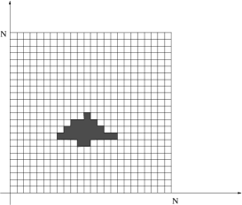
Figure 1:

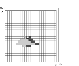
Figure 2:

Figure 3:

Consider now the evolution at the subsequent instant of time, namely after having progressed by a unit of time. Adding one point, $N\to N+1$, does produce an average geometry of a three sphere of radius $N+1$ instead of $N$. In the average, it is therefore like having added $4\pi N^{2}$ “points”, or unit cells. Remember that we work always with an infinite number of cells in an unspecified number of dimensions; when we talk of universe in three dimensions within a region of a certain radius, we just talk of the dominant geometry. Let’s suppose the position of the wave packet jumps by steps (two cells) back, as illustrated in figure 3. Namely, as time, and consequently also the radius of the universe, progresses by one unit, the packet moves at higher speed, jumping by two units. Compare this case with the case in which the packet jumps by just one unit, as in figure 3. The entropy of this latter configuration, intermediate between the first and second one, cannot be very different from the one of the second configuration, figure 3, in which the packet jumps by two steps, because that was supposed to be the dominant configuration at time $N+1$, and therefore the one of maximal entropy. Indeed, by “continuity” it must interpolate between step 2 and the configuration at time $N$, that was also supposed to be a configuration of maximal entropy. Therefore, the actual appearance of the universe at time $N+1$ must be somehow a superposition of the configurations 2 and 3, thereby contradicting our hypothesis that the wave packet is non-dispersive . Therefore, the wave packet cannot jump by two steps, and we conclude that the maximal speed allowed is that of expansion of the radius of the universe itself, namely, $c$.

It is too early here to discuss the actual existence in this scenario of degrees of freedom that can be interpreted as photons. In order to do this we must pass to a representation on the continuum, where, as discussed in [1], it corresponds to a string scenario. Here we just anticipate that, according to this theoretical framework, the reason why we have a universal bound on the speed of light is therefore that light carries what we call classical information. Information about whatever kind of event tells about a change of average entropy of the observed system, of the observer, and what surrounds and connects them too. The rate of transfer/propagation of information is therefore strictly related to the rate of variation of entropy. Variation of entropy is what gives the measure of time progress in the universe. Any carrier of information that “jumps” steps of the evolution of the universe, going faster than its rate of entropy variation, becomes therefore dispersive, looses information during its propagation. Light must therefore propagate at most at the rate of expansion of space-time (i.e. of the universe itself). Namely, at the rate of the space/time conversion, $c$.

5.2 The Lorentz boost

Let’s now consider physical systems that can be identified as “massive particles”, i.e. let us assume that there are local superpositions of configurations which are interpreted as travelling at speeds always lower than $c$. Since the phase space has a multiplicative structure, and entropy is the logarithm of the volume of occupation in this space, it is possible to separate for each such a system the entropy into the sum of an internal, “rest” entropy, and an external, “kinetic” entropy. The first one refers to the structure of the system in itself, that can be a particle or an entire laboratory. A point-like particle is an extended object of which we neglect the geometric structure. The second one refers to the relation/interaction of this system with the environment, the external world: its motion, the accelerations and external forces it experiences, etc.

Let us for a moment abstract from the fact that the actual configuration of the universe implied by 2.20 at any time describes a curved space. In other words, let’s neglect the so called “cosmological term”. This approximation can make sense at large $N$, as is the case of the present-day physics. This means at large age of the universe . Let us also assume we can just focus our attention on two observers sitting on two inertial frames, $A$ and $A^{\prime}$, moving at relative speed $v$, neglecting everything else. For what said above, $v<1$. An experiment is the measurement of some event that, owing to the fact that happening of something means changing of entropy and therefore is equivalent to a time progress, is perceived as having taken place during a certain interval of time. Let us consider an experiment, i.e. the detection of some event, taking place in the co-moving frame of $A^{\prime}$, as reported by both the observer at rest in $A$, and the one at rest in $A^{\prime}$ (from now on we will indicate with $A$, and $A^{\prime}$, indifferently the frame as well as the respective observer). Let’s assume we can neglect the space distance separating the two observers, or suppose there is no distance between them . For what we said above, such a detection amounts in observing the increase of entropy corresponding to the occurring of the event, as seen from $A$, and from $A^{\prime}$ itself. Since we are talking of the same event, the overall change of entropy will be the same for both $A$ and $A^{\prime}$. One would think there is an “absolute” time interval, related to the evolution of the universe corresponding to the change of entropy due to the event under consideration. However, the story is rather different as soon as we consider time measurements of this event, as reported by the two observers, $A$ and $A^{\prime}$. The reason is that the two observers will in general attribute in a different way what amount of entropy change has to be considered a change of entropy of the “internal” system, and which amount refers to an “external” change. Proper time measurements have to do with the internal change of entropy. For instance, consider the entropy of all the configurations contributing to form, say, a clock. The part of phase space describing the uniform motion of this clock will not be taken into account by an observer moving together with the clock, as it will not even be measurable. This part will however be considered by the other observer. Therefore, when reporting measurements of time intervals made by two clocks, one co-moving with $A$, and one seen by $A$ to be at rest in $A^{\prime}$, owing to a different way of attributing elements within the configurations building up the system, between “internal” and “external”, we will have in general two different time measurements. Let us indicate with $\Delta S$ the change of entropy as is observed by $A$. We can write:

$$\Delta S\,(\equiv\Delta S(A)) = \Delta S({\rm internal}\,=\,{\rm at\,rest})\,+\,\Delta S({\rm external})$$ (5.38)

$$= \Delta S(A^{\prime})\,+\,\Delta S_{\rm Kinetic}(A)\,,$$ (5.39)

with the identifications $\Delta S({\rm internal}\,=\,{\rm at\,rest})\equiv\Delta S(A^{\prime})$ and $\Delta S({\rm external})\equiv\Delta S_{\rm Kinetic}(A)$. In section 2.2 we discussed how the entropy of a three sphere is proportional to $N^{2}=E^{2}$. This is therefore also the entropy of the average, classical universe, that in the continuum limit, via the identification of total energy with time, can be written as:

$$S\;\propto\;\left(c{\cal T}\right)^{2}\,,$$ (5.40)

where ${\cal T}$ is the age of the universe. This relation matches with the Hawking’s expression of the entropy of a black hole of radius $r=c{\cal T}$ [7, 8]. It is not necessary to write explicitly the proportionality constant in (5.40), because we are eventually interested only in ratios of entropies. During the time of an event, $\Delta t$, the age of the universe passes from ${\cal T}$ to ${\cal T}+\Delta t$, and the variation of entropy, $\Delta S=S({\cal T}+\Delta t)-S({\cal T})$, is:

$$\Delta S\;\propto\;\left(c\Delta t\right)^{2}\,+\,c^{2}{\cal T}^{2}\left({2\Delta t\over{\cal T}}\right)\,.$$ (5.41)

The first term corresponds to the entropy of a “small universe”, the universe which is “created”, or “opens up” around an observer during the time of the experiment, and embraces within its horizon the entire causal region about the event. The second term is a “cosmological” term, that couples the local physics to the history of the universe. The influence of this part of the universe does not manifest itself through elementary, classical causality relations within the duration of the event, but indirectly, through a (slow) time variation of physical parameters such as masses and couplings, (we refer to [2] for a discussion of the time dependence of masses and couplings. See also [9]). In the approximation of our abstraction to the rather ideal case of two inertial frames, we must neglect this part, concentrating the discussion to the local physics. In this case, each experiment must be considered as a “universe” in itself. Let’s indicate with $\Delta t$ the time interval as reported by $A$, and with $\Delta t^{\prime}$ the time interval reported by $A^{\prime}$. In units for which $c=1$, and omitting the normalization constant common to all the expressions like 5.40 , we can therefore write:

$$\Delta S(A)\rightarrow\langle\Delta S(A)\rangle\approx(\Delta t)^{2}\,,$$ (5.42)

whereas

$$\Delta S(A^{\prime})\rightarrow\langle\Delta S(A^{\prime})\rangle\approx(\Delta t^{\prime})^{2}\,,$$ (5.43)

and

$$\Delta S_{\rm Kinetic}(A)~{}=~{}(v\,\Delta t)^{2}\,.$$ (5.44)

These expressions have the following interpretation. As seen from $A$, the total increase of entropy corresponds to the black hole-like entropy of a sphere of radius equivalent to the time duration of the experiment. Since $v=c=1$ is the maximal “classical” speed of propagation of information, all the classical information about the system is contained within the horizon set by the radius $c\Delta t=\Delta t$. However, when $A$ attempts to refer this time measurement to what $A^{\prime}$ could observe, it knows that $A^{\prime}$ perceives itself at rest, and therefore it cannot include in the computation of entropy also the change in configuration due to its own motion (here it is essential that we consider inertial systems, i.e. constant motions). “$A$” separates therefore its measurement into two parts, the “internal one”, namely the one involving changes that occur in the configuration as seen at rest by $A^{\prime}$ (a typical example is for instance a muon’s decay at rest in $A^{\prime}$), and a part accounting for the changes in the configuration due to the very being $A^{\prime}$ in motion at speed $v$. If we subtract the internal changes, namely we think at the system at rest in $A^{\prime}$ as at a point without meaningful physics apart from its motion in space , the entire information about the change of entropy is contained in the “universe” given by the sphere enclosing the region of its displacement, $v^{2}(\Delta t)^{2}~{}=~{}\Delta S_{\rm Kinetic}(A)$. In other words, once subtracted the internal physics, the system behaves, from the point of view of $A$, as a universe which expands at speed $v$, because the only thing that happens is the displacement itself, of a point otherwise fixed in the local universe (see figure 4).

Figure 4: During a time $\Delta t$, the pure motion “creates” a universe with an horizon at distance $\Delta x=v\Delta t$ from the observer. As seen from the rest frame, this part of the physical system does not exist. The “classical” entropy of this region is given by the one of its dominant configuration, i.e. it corresponds to the entropy of a black hole of radius $\Delta x$.

Inserting expressions 5.42–5.44 in 5.39 we obtain:

$$(\Delta t)^{2}~{}=~{}{(\Delta t^{\prime})^{2}\over 1-v^{2}}\,,$$ (5.45)

that is:

$$\Delta t~{}=~{}{\Delta t^{\prime}\over\sqrt{1-v^{2}}}\,.$$ (5.46)

The time interval as measured by $A$ results to be longer by a factor $(\sqrt{1-v^{2}})^{-1}$ than as measured by $A^{\prime}$. In this argument the bound on the speed of information, and therefore of light, enters when we write the variation of entropy of the “local universe” as $\Delta S=(c\Delta t)^{2}$. If $c\to\infty$, namely, if within a finite interval of time an infinitely extended causal region opens up around the experiment, both $A$ and $A^{\prime}$ turn out to have access to the full information, and therefore $\Delta t=\Delta t^{\prime}$. This means that they observe the same overall variation of entropy.

5.2.1 the space boost

In this framework we obtain in quite a natural way the Lorentz time boost. The reason is that, for us, time evolution is directly related to entropy change, and we identify configurations (and geometries) through their entropy. The space length is somehow a derived quantity, and we expect also the space boost to be a secondary relation. Indeed, it can be easily derived from the time boost, once lengths and their measurements are properly defined. However, these quantities are less fundamental, because they are related to the classical concept of geometry. We could produce here an argument leading to the space boost. However, this would basically be a copy of the classical derivation within the framework of special relativity. The derivation of the time boost through entropy-based arguments opens instead new perspectives, allowing to better understand where relativity ends and quantum physics starts. Or, to better say, it provides us with an embedding of this problem into a scenario that contains both these aspects, relativity and quantization, as particular cases, to be dealt with as useful approximations.

5.3 General time coordinate transformation

Lorentz boosts are only a particular case of the general coordinate transformation, obtained within the context of General Relativity; in that case the measure of time lengths is given by the time-time component of the metric tensor. In the absence of mixing with space boosts, i.e., with a diagonal metric, we have:

$$(ds)^{2}~{}=~{}g_{00}(dt)^{2}\,.$$ (5.47)

As the metric depends on the matter/energy content through the Einstein’s Equations:

$${\cal R}_{\mu\nu}-{1\over 2}g_{\mu\nu}{\cal R}\,=\,8\pi G_{N}T_{\mu\nu}\,,$$ (5.48)

$g_{00}$ can be computed when we know the energy of the system. For instance, in the case of a particle of mass $m$ moving at constant speed $v$ (inertial motion), the energy, the “external” energy, is the kinetic energy ${1\over 2}mv^{2}$, and we recover the $v^{2}$-dependence of the Lorentz boost .

In the simple case of the previous section, we have considered the physical system of the wave packet as decomposed into a part experiencing an “internal” physics, and a part which corresponds to the point of view of the center of mass, that is a part in which the complex internal physics is dealt with as a point-like particle. The Lorentz boost has been derived as the consequence of a transformation of entropies. Indeed, our coordinate transformation is based on the same physical grounds as the usual transformation of General Relativity, based on a metric derived from the energy tensor. Let us consider the transformation from this point of view: although imprecise, the approach through the linear approximation helps to understand where things come from. In the linear approximation, where one keeps only the first two terms of the expansion of the square-root $\sqrt{1-v^{2}/c^{2}}$, the Lorentz boost can be obtained from an effective action in which in the Lagrangian appear the rest and the kinetic energy. These terms correspond to the two terms on the r.h.s. of equation 5.39. Entropy has in fact the dimension of an energy multiplied by a time . Approximately, we can write:

$$\Delta S~{}\simeq~{}\Delta E\Delta t\,,$$ (5.49)

where $\Delta E$ is either the kinetic, or the rest energy. The linear version of the Lorentz boost is obtained by inserting in (5.49) the expressions $\Delta E_{rest}=m$ and $\Delta E_{kinetic}={1\over 2}mv^{2}$. In this case, the linearization of entropies lies in the fact that we consider the mass a constant, instead of being the full energy of the “local universe” contained in a sphere of radius $\Delta t$, i.e. the energy (mass) of a black hole of radius $\Delta t$: $m=\Delta E=\Delta t/2$. In our theoretical framework, the general expression of the time coordinate transformation is:

$$(\Delta t^{\prime})^{2}~{}=~{}\langle\Delta S^{\prime}(t)\rangle\,-\,\langle\Delta S^{\prime}_{external}(t)\rangle\,.$$ (5.50)

Here $\Delta S^{\prime}(t)$ is the total variation of entropy of the “primed” system as measured in the “unprimed” system of coordinates: $\langle\Delta S^{\prime}(t)\rangle\,=\,(\Delta t)^{2}$. We can therefore write expression 5.50 as:

$$(\Delta t^{\prime})^{2}~{}=~{}\left[1-\mathcal{G}(t)\right](\Delta t)^{2}\,,$$ (5.51)

where:

$$\mathcal{G}(t)~{}\stackrel{{\scriptstyle\mathrm{def}}}{{=}}~{}{\Delta S^{\prime}_{external}(t)\over(\Delta t)^{2}}\,.$$ (5.52)

With reference to the ordinary metric tensor $g_{\mu\nu}$, we have:

$$\mathcal{G}(t)~{}=~{}1-g_{00}\,.$$ (5.53)

$\Delta S^{\prime}_{external}(t)$ is the part of change of entropy of $A^{\prime}$ referred to by the observer $A$ as something that does not belong to the rest frame of $A^{\prime}$. It can be the non accelerated motion of $A^{\prime}$, as in the previous example, or more generally the presence of an external force that produces an acceleration. Notice that the coordinate transformation 5.51 starts with a constant term, 1: this corresponds to the rest entropy term expressed in the frame of the observer. For the observer, the new time metric is always expressed in terms of a deviation from the identity.

By construction, 5.52 is the ratio between the metric in the system which is observed and the metric in the system of the observer. From such a coordinate transformation we can pass to the metric of space-time itself, provided we consider the coordinate transformation between the metric $g^{\prime}$ of a point in space-time, and the metric of an observer which lies on a flat reference frame, whose metric is expressed in flat coordinates. We have then:

$$1\,-\,\mathcal{G}(t)~{}=~{}{g_{00}^{(\prime)}\over g^{(0)}_{00}\,=\eta_{00}=1}\,.$$ (5.54)

As soon as this has been clarified, we can drop out the denominator and we rename the primed metric as the metric tout court.

5.4 General Relativity

Once the measurement of lengths is properly introduced, as derived from a measurement of configurations along the history of the system, it is possible to extend the relations also to the transformation of space lengths. This gives in general the components of the metric tensor as functions of entropy and time. In classical terms, whenever this reduction is possible, this can be rephrased into a dependence on energy (energy density) and time. They give therefore a generalized, integrated version of the Einstein’s Equations. Let’s see this for the time component of the metric. We want to show that the metric $g_{00}$ of the effective space-time corresponds to the metric of the distribution of energy in the classical space, i.e., in the classical limit of effective three-dimensional space as it arises from 2.20. This will mean that the geometry of the motion of a particle within this space is the geometry of the energy distribution. In particular, if the energy is distributed according to the geometry of a sphere, so it will be the geometry of space-time in the sense of General Relativity. To this regard, we must remember that:

${\rm i})$ All these arguments make only sense in the “classical limit” of our scenario, namely only in an average sense, where the universe is dominated by a configuration that can be described in classical geometric terms. It is in this limit that the universe appears as three dimensional. Configurations which are in general non three-dimensional, non-geometric, possibly tachyonic, and, in any case, configurations for which General Relativity and Einstein Equations don’t apply, are covered under the “un-sharping” relations of the Uncertainty Principle. All of them are collectively treated as “quantum effects”;

${\rm ii})$ In the classical limit, nothing travels at a speed higher than $c$. As during an experiment no information comes from outside the local horizon set by the duration of the experiment itself, to cause some (classical) effects on it, any consideration about the entropy of the configuration of the object under consideration can be made “local” (tachyonic effects are taken into account by quantization). That means, when we consider the motion of an object along space we can just consider the local entropy, which depends on, and is determined by, the energy distribution around the object.

Having these considerations in mind, let us consider the motion of a particle, or, more precisely, a non-dispersive wave-packet, in the three-dimensional, classical space. Consider to perform a (generally point-wise) coordinate transformation to a frame in which the metric of the energy distribution external to the system intrinsically building the wave packet in itself is flat, or at least remains constant. As seen from this set of frames, along the motion there is no change of the (local) entropy around the particle, and the right hand side of 5.52 vanishes, implying that also the metric of the motion itself remains constant (remember that 5.52 in this case gives the ratio between metrics at different points/times). This means that the metric of the energy distribution and the metric of the motion are the same, and proves the equivalence of 5.50 and 5.52 with the Einstein’s equations 5.48. If on the other hand we keep the frame of the observer fixed, and we ask ourselves what will be the direction chosen by the particle in order to decide the steps of its motion, the answer will be: the particle “decides” stepwise to go in the direction that maximizes the entropy around itself. Let us consider configurations in which the only property of particles is their mass (no other charges), so that entropy is directly related to the “energy density” of the wave packet. In this case, between the choice of moving toward another particle, or far away, the system will proceed in order to increase the energy density around the particle. Namely, moving the particle toward, rather than away from, the other particle, in order to include in its horizon also the new system. This is how gravitational attraction originates in this theoretical framework.

In order to deal with more complicated cases, such as those in which particles have properties other than just their mass (electro-magnetic/weak/strong charge), we need a more detailed description of the phase space. In principle things are the same, but the appropriate scenario in which all these aspects are taken into account is the one in which these issues are phrased and addressed within a context of (quantum) String Theory. This analysis, first presented in Ref. [9], is discussed in detail in Ref. [2].

5.5 The metric around a black hole

Let us consider once more the general expression relating the evolution of a system as is seen by the system itself, indicated with $A^{\prime}$, and by an external observer, $A$, expressions 5.38 and 5.39. In the large-scale, classical limit, the variations of entropy $\Delta S(A)$ and $\Delta S(A^{\prime})$ can be written in terms of time intervals, as in 5.42 and 5.43, in which $t$ and $t^{\prime}$ are respectively the time as measured by the observer, and the proper time of the system $A^{\prime}$. In this case, as we have seen expression 5.39 can be written as $(\Delta t^{\prime})^{2}=(\Delta t)^{2}\,-\,\langle\Delta S^{\prime}_{\rm external}(t)\rangle$ (see expression 5.50), and the temporal part of the metric is given by:

$$g_{00}~{}=~{}{\langle\Delta S^{\prime}_{\rm external}(t)\rangle\over(\Delta t)^{2}}\,-\,1\,.$$ (5.55)

As long as we consider systems for which $g_{00}$ is far from its extremal value, expression 5.55 constitutes a good approximation of the time component of the metric. However, a black hole does not fall within the domain of this approximation. According to its very (classical) definition, the only part we can probe of a black hole is the surface at the horizon. In the classical limit the metric at this surface vanishes: $g_{00}\to 0$ (an object falling from outside toward the black hole appears to take an infinite time in order to reach the surface). This means,

$$\langle\Delta S_{\rm external}\rangle~{}\approx~{}\propto\,\left(\Delta t\right)^{2}\,.$$ (5.56)

However, in our set up time is only an average, “large scale” concept, and only in the large scale, classical limit we can write variations of entropy in terms of progress of a time coordinate as in 5.42 and 5.43. The fundamental transformation is the one given in expressions 5.38, 5.39, and the term $g_{00}$ has only to be understood in the sense of:

$$\Delta S(A^{\prime})\,\longrightarrow\,\langle\Delta S(A^{\prime})\rangle\,\equiv\,\Delta t^{\prime}g_{00}\Delta t^{\prime}\,.$$ (5.57)

The apparent vanishing of the metric 5.55 is due to the fact that we are subtracting contributions from the first term of the r.h.s. of expression 5.39, namely $\Delta S(A^{\prime})$, and attributing them to the contribution of the environment, the world external to the system of which we consider the proper time, the second term in the r.h.s. of 5.39, $\Delta S_{\rm external}(A)$. Any physical system is given by the superposition of an infinite number of configurations, of which only the most entropic ones (those with the highest weight in the phase space) build up the classical physics, while the more remote ones contribute to what we globally call “quantum effects”. Therefore, taking out classical terms from the first term, $\Delta S(A^{\prime})$, the “proper frame” term, means transforming the system the more and more into a “quantum system”. In particular, this means that the mean value of whatever observable of the system will receive the more and more contribution by less localized, more exotic, configurations, thereby showing an increasing quantum uncertainty. In particular, the system moves toward configurations for which $\Delta x\rightarrow\gg 1/\Delta p$. Indeed, one never reaches the condition of vanishing of 5.57, because, well before this limit is attained, also the notion itself of space, and time, and three dimensions, localized object, geometry, etc…, are lost. The most remote configurations in general do not describe a universe in a three-dimensional space, and the “energy” distributions are not even interpretable in terms of ordinary observables. At the limit in which we reach the surface of the horizon, the black hole will therefore look like a completely delocalized object [4].

5.6 Natural or real numbers?

The approach we are proposing, and the fact that from the collection of binary codes we arrive to the structures of our physical world, implies a question about what is after all the world we experience. We are used to order our observations according to phenomena that take place in what we call space-time. An experiment, or, better, an observation (through an experiment), any perception in itself, basically consists in realizing that something has changed: our “eyes” have been affected by something, that we call “light”, that has changed their configuration (molecular, atomic configuration). This light may carry information about changes in our environment, that we refer either to gravitational phenomena, or to electromagnetic ones, and so on… In order to explain them we introduce energies, momenta, “forces”, i.e. interactions, and therefore we speak in terms of masses, couplings etc… However, all in all, what all these concepts refer to is a change in the “geometry” of our environment, a change that “propagates” to us, and eventually results in a change in our brain, the “observer”. But what is after all geometry, other than a way of saying that, by moving along a path in space, we will encounter or not some modifications? Assigning a “geometry” is a way of parametrizing modifications. Is it possible then to invert the logical ordering from reality to its description? Namely, can we argue that what we interpret as energy, or geometry, is simply a code of information . Something happens, i.e. time passes, when some code changes. Viewed in this way, it is not a matter of mapping physical degrees of freedom into a language of abstract codes, but the other way around, namely: perhaps the deepest reality is “information”, that we arrange in terms of geometries, energies, particles, fields, and interactions. When we “see” the universe, we interpret the codes in terms of maps, from a space of “energies” to a target space, that take the “shape” of what we observe as the physical reality. From this point of view, information is not just something that transmits knowledge about what exists, but it is itself the essence of what exists, and the rationale of the universe is precisely that it ultimately is the whole of rationale. The quantum (in the sense of indeterministic) nature of the universe is then the consequence of being any observable not just a code but a collection, a superposition, of codes.

Reducing everything to a collection of binary codes means reducing everything to a discrete description in terms of natural numbers, i.e. to saying that the whole of rationale is numerable. One may wonder whether natural numbers are enough to encode all the information of the universe. At first sight, one would say that real numbers say “more”, allow to express more information. Moreover, they appear to be “real” in the true sense of something existing in nature. For instance, one can think to draw with the pencil a circle and a diameter. Then, one has physically realized two lines of lengths that don’t stay in a ratio expressible as a rational number. However here the point is: what is really about the microscopical nature of these two drawings? At the microscopical level, at the scale of the Planck length, the notion of space itself is so fuzzy to be practically lost. In our scenario, an analysis of the superposition of configurations tells us that, before reaching this scale, remote configurations, whose contribution is usually collected under the Heisenberg’s Uncertainty, count more and more. In other words, the world is no more classical but deeply quantum mechanical, to the point that the uncertainty in the length of the two lines doesn’t allow us to know whether their ratio is a real or a rational number. In this sense, this analysis provides further support to an old idea which goes back to Konrad Zuse, that all the information of the universe is expressible through natural numbers, and, as a consequence, the discrete description of the universe, and in particular of space-time, is not just an approximation, but indeed the most fundamental one can think about. After all, real numbers are introduced in mathematics through definitions and procedures, whose informational content can be “written” as a text with a computer program. This means that, as a matter of pure information content, real numbers can be introduced via natural numbers.

References

- [1] A. Gregori, Combinatorics, observables, and String Theory, arXiv e-prints (2011) arXiv:1103.4000.
- [2] A. Gregori, Combinatorics, observables, and String Theory, part II, arXiv e-prints (2011) arXiv:1103.3998.
- [3] A. Gregori, On the Critical Temperatures of Superconductors: a Quantum Gravity Approach, arXiv e-prints (July, 2010) arXiv:1007.3731.
- [4] A. Gregori, Is the Universe the only existing Black Hole?, ArXiv e-prints (June, 2010) 1006.5826.
- [5] A. Gregori, A note on the phases of natural evolution, arXiv:0712.0074 [physics.gen-ph].
- [6] M. Rabinowitz, n-dimensional gravity: Little black holes, dark matter, and ball lightning, Int. J. Theor. Phys. 40 (2001) 875–901, astro-ph/0104026.
- [7] J. M. Bardeen, B. Carter, and S. W. Hawking, The Four laws of black hole mechanics, Commun. Math. Phys. 31 (1973) 161–170.
- [8] J. D. Bekenstein, Black holes and entropy, Phys. Rev. D7 (1973) 2333–2346.
- [9] A. Gregori, An entropy-weighted sum over non-perturbative vacua, arXiv:0705.1130 [hep-th].
- [10] L. D. Landau and E. M. Lifshitz, The Classical Theory of Fields.