IN SEARCH OF RANDOM UNCORRELATED PARTICLE MOTION (RUM) IN A SIMPLE RANDOM FLOW FIELD

email: mike.reeks@ncl.ac.uk, soldati@uniud.it, luca.fabbro@uniud.it

ABSTRACT
DNS studies of dispersed particle motion in isotropic homogeneous turbulence [1] have revealed the existence of a component of random uncorrelated motion (RUM) dependent on the particle inertia $\tau_{p}$(normalised particle response time or Stoke number). This paper reports the presence of RUM in a simple linear random smoothly varying flow field of counter rotating vortices where the two-particle velocity correlation was measured as a function of spatial separation.Values of the correlation less than one for zero separation indicated the presence of RUM. In terms of Stokes number, the motion of the particles in one direction corresponds to either a heavily damped $\left(\tau_{p}<0.25\right)$ or lightly damped $\left(\tau_{p}>0.25\right)$ harmonic oscillator. In the lightly damped case the particles overshoot the stagnation lines of the flow and are projected from one vortex to another (the so-called sling-shot effect). It is shown that RUM occurs only when $\tau_{p}>0.25$, increasing monotonically with increasing Stokes number. Calculations of the particle pair spatial distribution function show that equilibrium of the particle concentration field is never reached, the concentration at zero separation increasing monotonically with time. This is consistent with the calculated negative values of the average Liapounov exponent (finite compressibility) of the particle velocity field.

1 INTRODUCTION

Turbulent structures play a crucial role in many particle/fluid processes in the environment and industry: in powder production, combustion, and the formation and growth of PM10 particulates in the atmosphere. An area of much investigation is the mechanism for warm-rain initiation and in particular the way droplet interaction with the small scales of turbulence in clouds influence the droplet size distribution. The current consensus is that the turbulence demixes the particles leading to a much enhanced collision rate (i.e. much greater than that based on passive scalar motion[2],[3]). Our only particular interest in this subject is motivated by the processes of turbulent agglomeration and deagglomeration of a aerosols released in a steam generator tube rupture in a PWR. Early experiments and simulations[4] have shown that this demixing reaches a maximum when the particle response time is typical of the timescale of the turbulent structure (i.e particle Stokes numbers $\sim$ 1), the suspended particles being observed to segregate into regions of high straining rate in between the regions of vorticity. In addition Maxey and his co-workers[5],[6] showed that the gravitational settling of particles in homogeneous turbulence was enhanced due preferential sweeping in the direction of gravity as particles interweave through turbulent structures in the flow. Since then there have been numerous studies to understand and quantify this segregation process. Of particular note have been the seminal studies by Collins et al.[7] and Wang et al.[8] to quantify the influence of segregation on relative dispersion (two particle dispersion) and on particle agglomeration and the recent work of Bec [9] who expressed the clustering of particle in terms of its fractal dimension and showed how this was related to the Liapounov exponents of the particle phase space distribution. Even more recently Vassilicos[10] has shown that the clustering is strongly related to the acceleration stagnation points in the flow as they are swept by the large scale motions of the turbulence.

This paper is not directly concerned with the clustering but with an intrinsic property of the motion of inertial particles in flow fields that are spatially random but smoothly varying. Simonin et al. [1] have observed that the spatial velocity field resulting from the motion of suspended particles in DNS isotropic homogeneous turbulence consists of two components: a smoothly (continuous) velocity field that accounts for all particle-particle and fluid-particle two point spatial correlations (they referred to this components as the mesoscopic Eulerian particle velocity field (MEPVF)); and a spatially uncorrelated component which we will refer to here as RUM (the component of random uncorrelated motion) whose contribution to the particle kinetic energy increases as the particle inertia increased. Simonin et al [1] attribute this feature to the ability of the particles with inertia to retain their memory of their interaction with very distant, and statistically independent eddies in the flow field. The flow field in their DNS of homogeneous isotropic turbulence as with real turbulence is complicated with many scales of spatial and temporal existence. In our study, the results of which we present here, we show the presence of RUM in a much simpler flow field of counter rotating vortices and in so doing are able to examine the properties of RUM in relation to the particle interactions with simple structures. The flow field we have used has been used before in studies of particle clustering [11] and in particular with the measurement of the particle compressibility and intermittency. Our eventual aim is to show how these properties are related to the occurrence of RUM

2 DESCRIPTION OF CARRIER FLOW FIELD

This flow field and its properties we have described in detail elsewhere [11] but for completeness we shall include a brief description here. We consider dispersion in a simple homogeneous turbulent flow field composed of pairs of counter rotating vortices which are periodic in both the x,y directions with the same periodicity. Each lattice cell (the basic periodic element) contains a pair of counter-rotating vortices in both the x,y orthogonal directions and is constructed from a linear symmetric straining flow field in the manner shown in Figure 1

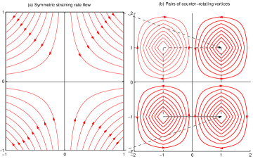
a) Generation from symmetric strain rate flow

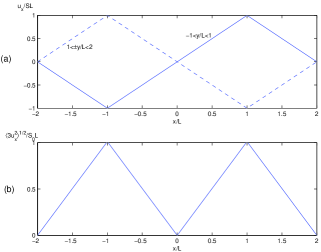
b) Carrier flow velocity and rms velocity in x-direction

Figure 1: Generation of carrier flow field velocity and its $x-$variation within a flow lattice cell

So starting from an initial symmetric straining flow pattern of width $2L$ in both the $x,y$ directions (see Fig. 1(a) ), this pattern is repeated front to back in both the $x,y$ directions with a strain rate $S$ drawn from a uniform distribution $\left[0,S_{0}\right]$. We note that each quadrant of this straining rate pattern in Fig.1(a) is a quadrant of one of the two pairs of counter-rotating vortices formed within the lattice cell in Fig.1(b). As shown in Fig.1(a), the flow velocity $u_{x}$ in the $x-$direction has a linear saw-tooth profile $U(x)$, with a slope of constant magnitude $S$ but with a change in sign across the $y$-centre line of a vortex where the maximum and minimum values $\pm SL/2$ of $U(x)$ are located: across the $x$-centre line, $u_{x}$ changes to $-U(x)$ as shown in Fig.1(b), consistent with the change in direction of the streamlines shown in Fig.1(a). The flow velocity $u_{y}$ in the $y$-direction at $(x,y)$ is $-U(y)$ to preserve continuity of flow through out. This cellular flow pattern of counter-rotating vortices so formed, persists for a fixed life-time selected from an exponential distribution with a decay time of $S_{0}^{-1}$, at the end of which time, a fresh flow field is generated with new values of the life-time and $S$ and the origin of the pattern at the same time shifted by random displacements in both the $x$ and $y$-directions, drawn independently from a uniform distribution $\left[0,2L\right]$. This makes the average flow homogeneous with zero mean in the $x-$ $y$-directions. The important feature of this randomized flow field is that the equations of motion of an individual particle in both the $x,y$-directions are linear and independent of one another (other than through the maximum length of time a particle can experience a particular value of the straining of the flow in either the $x$- or $y$-directions before it changes sign). With respect to the centre (stagnation point) of a symmetric straining flow pattern (see Fig.1(a)), the flow velocity within that flow region is given by :

$$u_{x}=+Sx\;;\;u_{y}=-Sy\;\;(-L\leq x\leq L,\>-L\leq y\leq L)$$ (2.1)

The flow field so generated turns out to be homogeneous and stationary but not isotropic. It has the interesting property that the Lagrangian fluid point rms velocity (along its trajectory) is different from its value at a fixed point (Eulerian).

2.1 Particle equations of motion

Based on Stokes drag, the particle equation of motion is

$$\ddot{x}_{i}+\tau_{p}^{-1}\dot{x}_{i}+(-1)^{i+1}\tau_{p}^{-1}Sx_{i} = 0$$ (2.2)

$$-L\leq x_{i}\leq L\;(i=1,2)(x_{1}=x,x_{2}=y)$$

where $x_{i}$ is measured from a stagnation point. For convenience we normalize $x_{i}$ on $L$ and express the particle response time $\tau_{p}$ and strain rate $S$ in units of $S_{0}^{-1}$ so $\tau_{p}$ is the particle Stokes number and in this case $S$ is drawn from a uniform distribution $\wp\left[0,1\right]$. We note that when the strain rate in the $x,y$ directions the $x,y$ equations are those of a damped simple harmonic oscillator and as a consequence there are two types of motion, namely heavily damped for $\tau_{p}<0.25$ and lightly damped for $\tau_{p}>0.25$. This has some bearing on the motion of the particle within these vortices. For heavily damped motion, a particle remains trapped within a vortex but approaches the extremity (the stagnation region) in a manner which decreases exponentially with time. On the other hand for lightly damped motion the particle can escape the vortex or overshoot into an adjacent vortex, and in so doing overshoot into the adjacent vortex to that. This has been referred to as the sling shot effect and it is this type of motion that gives rise to RUM. Both these types of behaviour are illustrated in Figure 2 (a) and (b) for particle response times $\tau_{p}=0.1$ (heavily damped) and $\tau_{p}=1$ (lightly damped).

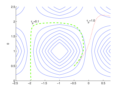
Figure 2: Particle trajectories in vortices: $\tau_{p}$=0.1 , heavily damped; $\tau_{p}=1,$lightly damped

Figure3 also show the corresponding values of components $J_{11}$ and $J_{22}$ of the the unit deformation tensor $\mathbf{J}$ given by $\partial\mathbf{x}(\mathbf{x_{0},}t)/\partial\mathbf{x}_{0}$ where $\mathbf{x_{0}}$ is the position of the particle at some initial time say $t=0$. In this case we have set $J_{ij}(0)=\delta_{ij}$. The equations of motion for $J_{ij}$ are obtained from the particle equations of motion by partial differentiation wrt $x_{0,i}$ giving

$$\ddot{J_{ij}}+\tau_{p}^{-1}\dot{J}_{ij}+(-1)^{i+1}\tau_{p}^{-1}SJ_{ij}=0$$ (2.3)

for which we choose the initial conditions $\dot{J}_{ij}=\partial u_{i}/\partial x_{j}=(-1)^{i+1}\tau_{p}^{-1}S\delta_{ij}$. This means that together with the initial conditions on $J_{ij}$ that $J_{ij}(t)=0$ for $i\neq j$ and that

$$J(t)=\left|\mathbf{J}\right|=J_{11}J_{22}$$ (2.4)

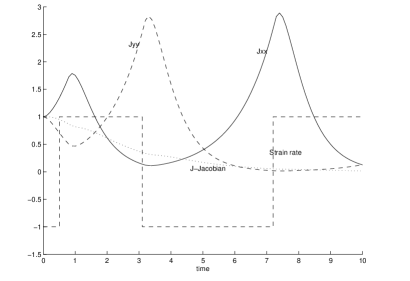
a) $St=0.1,\mbox{ heavilydamped}$

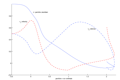
b) $St=1$., lightly damped

Figure 3: Compenents of the deformation tensor $\mathbf{J}$ and compression $\left|J\right|$along particle trajectories :

Note that in this linear system the equation of motion for $J(t)$ is the same as that for $x_{i}$ and that the components of $\mathbf{J}$ are dependent on the position of the particle only through the time at which the strain rate experienced by the particle changes sign. Fig 3(a) and (b) shows the corresponding values of $J(t)$ along the heavily damped and lightly damped (b) trajectories. In both cases the value of $J$ approaches zero as $t\rightarrow\infty$. However in the lightly damped case $J(t)$ passes through zero at intermediate times as the particle oscillates backwards and forwards across a stagnation line. In so doing the value of $J$ oscillates from $+ve$ to $-ve$, with the corresponding elemental volume rotating through $180^{0}$ as it passes through zero volume. Each time $J(t)$ passes through zero, the corresponding particle concentration becomes infinite instantaneously. This raises the possibility that such events may occur in real turbulent flows and that the process of particle dispersion could be a highly intermittent process associated with large deviations in the particle concentrations. It also indicates the conditions under which particle trajectories cross. That is given an initially uniform distribution of particle with velocities uniquely defines at each point by the local fluid velocity., as time elapses the particle velocity field is not uniquely defines at each point. This ultimately is the origin of RUM.

3 Calculation of RUM

We calculated RUM by measuring the contribution it makes to the particle kinetic energy (per unit mass). We did this by calculating the particle pair velocity correlation as a function of particle separation. In particular we calculated

$$R_{xx}(\Delta x)=\langle\textrm{v}_{x}^{(1)}(x,0)\textrm{v}_{x}^{(2)}(x+\Delta x,0)\rangle/\langle\textrm{v}_{x}^{2}\rangle$$ (3.5)

where $(1)$and $(2)$refer to two particles labelled (1) and $(2)$separated by a distance $\left[\Delta x,0\right]$and $\langle\rangle$is an average over all particle pairs for which the separation is $\Delta x$. We began with a fully mixed flow of particles with the local fluid velocity. Periodicity of the lattice cell dimensions means that initially for any integers $n$, and $m$,the initial particle velocity field satisfies the periodic boundary condition, $\mathbf{v}(x,y)=\mathbf{v}(x+4n,y+4m)$. Given this initial velocity field means that for any given particle trajectory $\mathbf{X}_{1}(\mathbf{x}_{1},t)$ there will be an identical particle trajectory $\mathbf{X}_{2}(x_{1}+4n,y+4m_{1})$, for which

$$\mathbf{X}_{2}(x_{1}+4n,y+4m_{1},t)=\mathbf{X}_{1}(\mathbf{x_{1}},t)+\mathbf{\Gamma};\>\mathbf{\Gamma}=(4n,4m)$$ (3.6)

That is two particle starting out from identical positions within any two lattice cells will experience the same relative displacement with respect to their initial positions and necessarily experience the same flow velocity at any given time even though the whole lattice is displaced randomly at each life time. This means that if we consider particles entering or leaving a fixed cell of lattice dimensions, any particle leaving the cell will be replaced by an identical particle at the opposite face whose velocity is identical to that of the particle leaving. Thus at any instant of time, the number of particles within the cell remains constant; only the concentration within the cell will change. Periodicity of the particle motion and homogeneity means further more that for the particle pair velocity correlation

$$\begin{array}[]{c}R_{xx}(\Delta x)=R_{xx}(-\Delta x)=R_{xx}(4-\Delta x)=R_{yy}(\Delta y)\\ =R_{yy}(-\Delta y)=R(4-\Delta y)\end{array}$$ (3.7)

Because the particle concentration is initially uniform, the particle pair correlation is identical to the Eulerian spatial velocity correlation which we can calculate directly, namely

$$R_{xx}(\Delta x)=\int_{lattice}u_{x}(x,y)u_{x}(x+\Delta x,y)dxdy/\langle u_{x}^{2}\rangle=\frac{1}{16}\int_{-1}^{3}\int_{-1}^{3}u_{x}(x,y)u_{x}(x+\Delta x,y)dxdy$$ (3.8)

After some labour, one arrives at the result

$$\begin{array}[]{cc}0\leq\Delta x\leq 2&\;R_{xx}(\Delta x)=\left[1-\frac{3}{2}\Delta x^{2}+\frac{1}{2}\Delta x^{3}\right]\\ 2\leq\Delta x\leq 4&R_{xx}(\Delta x)=\frac{9}{12}\left[12-16\Delta x+6\Delta x^{2}-\frac{2}{3}\Delta x^{3}\right]=\left[9-12\Delta x+\frac{9}{2}\Delta x^{2}-\frac{1}{2}\Delta x^{3}\right]\end{array}$$ (3.9)

These forms provide an independent check on our method of calculating the particle pair velocity correlation based on counting the number of particle pairs with a given separation . The method within the statistical error correctly reproduces the correlation coefficient for the particle initial uniform distribution (See Fig. 5)

a) St=0.1, time =10

b) St=0.1, time=40

c) St=1, time=10

d) St=1, time=40

e) St=10, time=10

f) St=10, time=40

Figure 4: Particle distributions at time $t=10$ and 40, for $St=0.1,1.,10$

Figure 4 shows the positions of $500$ particles initially distributed uniformally within a cell whose boundaries are coincident with a lattice cell initially but which remains fixed throughout the simulation, and for which periodic boundary conditions are applied at the edges of the cell to particles entering and leaving it. The resulting particle distributions in Figure4 are for a given random sequence of the straining rate$S$and lattice life time. The particular distributions shown are at times $t=10$ and $t=40$ for particle response times (Stokes nos.) of $\tau_{p}=0.1,1.0,10.$ We note first that the case of the intermediate response time $\tau_{p}=1$, exhibits the greatest degree of segregation, being markedly greater than the other two cases. Secondly the segregation increases with time and carries on indefinitely. Thirdly there is no identifiable self preserving pattern of segregation, nor does the segregation align with the local stagnation lines of the flow at any instant of time. In fact another random sequence of strain rates and lifetimes would lead to an entirely different pattern. The increasing segregation would lead to a lower fractal dimension and the increase of the particle pair concentration at zero separation values for the pair separation distribution function as shown in Figure 4 described below.

In calculating the correlation coefficient $R_{xx}(\Delta x)$for particle pair separation in the $x$-direction, the positions of $N$ particles within the domain $\left[0\leq\Delta x\leq 4\,,\,0\leq y\leq 4\right]$are evaluated as a function of time by first solving the set of equations of motion (2.2). The domain $\left[0\leq\Delta x\leq 4\,,\,0\leq y\leq 4\right]$is divided up into $10^{2}\times 10^{2}$ bins of $0.04$ dimension in both the $\Delta x,y$ directions, the $(m,n)$bin being the bin whose centre is at $\Delta x=$$0.04(m-\frac{1}{2}),y=0.04(n-\frac{1}{2})$ where $m,n=1,..100$. For each particle pair whose $y$- co-ordinates satisfy $0.04(n-1)<y<n0.04$ we evaluate the separation $\Delta x$. If $\Delta x>0$ we determine the value of $m$ for which $0.04(m-1)<\Delta x<m0.04$ and store the value $\textrm{v}_{x}^{(1)}(x,0)\textrm{v}_{x}^{(2)}(x+\Delta x,0)$ in the $(m,n)$bin. If $\Delta x<0$, we store these values in the $\left(m,n\right)$bin for which $0.04m<4-\Delta x<(m+1)0.04$. In this way, for all particle pairs whose $x-$position is $-2<x<2$ we cover the range $0\leq\Delta x\leq 4$. After sorting all particle pairs into suitable bins, we then repeat this procedure for $M$ realisations of the carrier flow and then sum the values of $\textrm{v}_{x}^{(1)}(x,0)\textrm{v}_{x}^{(2)}(x+\Delta x,0)$for all particle pairs within each bin and divide this by the number of particle pairs to give the average value $\left\langle\textrm{v}_{x}^{(1)}(x,0)\textrm{v}_{x}^{(2)}(x+\Delta x,0)\right\rangle$. In addition we calculate $\langle\textrm{v}_{x}^{2}\rangle$by summing $\textrm{v}_{x}^{2}$over all $N$ particles in the box and over $M$ realisations of the flow field and then dividing by $MN,$ finally to obtain $R_{xx}(\Delta x)$ using Eq.(3.5). For accuracy versus computation time we chose $N=10^{3}$ particles and $M=10^{3}$ realisations of the flow. At the same time as summing over the values $\textrm{v}_{x}^{(1)}(x,0)\textrm{v}_{x}^{(2)}(x+\Delta x,0)$ in all bins with the same value of $n$, we also summed the number of pairs in each bin and divided by $0.04$, to evaluate the particle pair distribution $g(\textrm{$\Delta x$})$which we normalised to unity by dividing the number of pairs within the domain $0\leq\Delta x\leq 4$. i.e.

$$\int_{0}^{4}g(\Delta x)d\Delta x=1$$

For each of values of $\tau_{p}=0.1,1,10$, Figure 5 shows the particle pair velocity correlation coefficient $R_{xx}(\Delta x)$ at time $t=20)$ as a function of the pair separation. These three curves are to be compared with the curve for the initial distribution given by Eq.(3.9). It is apparent that the case for $\tau_{p}=0.1$ is almost identical to the initial form of the pair separation correlation. For the other cases, the curves are noticeably different, with the most interesting property of all, that the extrapolated values for $\Delta x=0$are not unity as is the case of the initial pair correlation function and that of the case of $\tau=0.1$. This is most marked for $\tau_{p}=10$. The difference between the extrapolated value and unity represents the contribution of RUM to the particle kinetic energy. More revealing are the calculated values of RUM plotted against $\tau_{p}$ shown in Fig.6 for $t=20$. We note that there is no real measurable contribution from RUM until $\tau_{p}\geq 0.25$. For $\tau_{p}\leq 0.25$ all realisable states correspond to a sequence of heavily damped system with $\tau_{p}S$$\leq 0.25$: above $\tau_{p}=0.25$ the system behaves as a mixture of heavily damped and lightly damped harmonic oscillators. The threshold of $\tau_{p}=0.25$ for the occurrence of RUM, shows conclusively that RUM is associated with the behaviour of a lightly damped system in the manner described earlier.

Finally Figure 7 show the calculated values of the particle pair distribution function $g(x)$. Figure 7 (a) shows that for the 3 values of $\tau_{p}=0.1,1.0,10$ the maximum peak concentration $\Delta x=0$occurs at the intermediate values of $\tau_{p}=1.$. Fig7(b) shows peak distribution increasing with time for $\tau_{p}=1,$a result that is true for all values of $\tau_{p}$. We recall that these features are consistent with the segregation of particles shown in Figure 4

4 Summary and Concluding remarks

We have shown and measured a contribution to the particle kinetic energy from a component of random uncorrelated motion (RUM) of particles suspended in a simple random but smoothly varying flow field composed of counter rotating vortices. This feature has been observed in more complex flow. Depending upon the value of the particle response time $\tau_{p}$(Stokes number) the motion of the particles corresponds to that of a heavily or lightly damped harmonic oscillator. Within statistical error, RUM was only detected when the particle motion at some stage corresponded to a lightly damped oscillator in particular when $\tau_{p}\geq 0.25$. In this case the particles overshoot the stagnation lines in the flow and can pass form one vortex to another in the flow. This behaviour is consistent with the description given by Simonin et al.[1] who first observed RUM in particle motion in DNS isotropic homogeneous turbulence. There remains the possibility of linking RUM with the occurrence of singularities in the particle concentration flow field and to the intermittency in the particle flow filed. Simonin et al. [1] have developed a statistical approach to describing particle motion in these circumstances. They have considered RUM as a device for stabilising the segregation (the RUM acting as a pressure, the gradient of which acts in opposition to the force driving the segregation. Here we note that the segregation does not stabilise even though RUM is definitely present.

Figure 5: correlation coefficient $R_{xx}(X)$ at time $t=40$, where $X$is the $x$-separation of particle pairs; note that , $R_{xx}(X)$is symmetric $X=2$

Figure 6: RUM contribution to particle kinetic energy

Figure 7: Particle pair distribution $g(X)$, $X$= particle pair separation

References

- [1] Fevre P. , Simonin O and Squires K. D. 2005 Partitioning of particle velocities in gas-solid turbulent flows into a continuous field and a spatially uncorrelated random distribution; theoretical formalism and numerical study. J. Fluid Mech. 553, 1-46
- [2] Shaw R. A. 2003: Particle-turbulence interactions in atmospheric clouds Ann. Review of Fluid Mechanics 35, 183-227.
- [3] Falkovich G, Fouxon A.S. & Stepanov M. G. 2002. Acceleration of rain initiation by cloud turbulence Nature 419, 151-154
- [4] Crowe C.T. Chung J. N. & Troutt T. R.1993, Particulate Two phase Flow Ch 18 (ed. Roco, M. C) 626, Heinemann, Oxford.
- [5] Maxey M. R. 1987 The gravitational settling of aerosol particles in homogeneous turbulence and random flow fields. J. Fluid Mech. 174, 441-465
- [6] Wang L. P. and Maxey M. R. 1993 Settling velocity and concentration distribution of heavy particles in homogeneous isotropic turbulence. J. Fluid Mech. 256, 27-68
- [7] Sundaram S. & Collins L. R. 1997 Collision statistics in an isotropic particle-laden turbulent suspension. Part 1. Direct Numerical simulations. J. Fluid Mech. 335, 75-109
- [8] Lian-Ping Wang, Wexler, S., and Yong Zhou 1998 Statistical mechanical descriptions of turbulent coagulation Phys Fluids 10(10) 2647-2651
- [9] Bec, J. 2005 Multifractal concentrations of inertial particles in smooth random flow J. Fluid Mech. 528, 255-277
- [10] Chen, L. Goto, S., and Vassilicos, J. C. 2006 Turbulent clustering of stagnation points and inertial particles J. Fluid Mech.553 143-154
- [11] Reeks, M. W. 2004 Simulation of particle diffusion, segregation, and intermittency in turbulent flows IUTAM Symposium on Stimulation of Multiphase Flows, Argonne National Lab, Oct 4-7