The Delay Time Distribution of Type-Ia Supernovae from Sloan II

Abstract

We derive the delay-time distribution (DTD) of type-Ia supernovae (SNe Ia) using a sample of 132 SNe Ia, discovered by the Sloan Digital Sky Survey II (SDSS2) among 66,000 galaxies with spectral-based star-formation histories (SFHs). To recover the best-fit DTD, the SFH of every individual galaxy is compared, using Poisson statistics, to the number of SNe that it hosted (zero or one), based on the method introduced in Maoz et al. (2011). This SN sample differs from the SDSS2 SN Ia sample analyzed by Brandt et al. (2010), using a related, but different, DTD recovery method. Furthermore, we use a simulation-based SN detection-efficiency function, and we apply a number of important corrections to the galaxy SFHs and SN Ia visibility times. The DTD that we find has $4\sigma$ detections in all three of its time bins: prompt ($\tau<0.42$ Gyr), intermediate ($0.42<\tau<2.4$ Gyr), and delayed ($\tau>2.4$ Gyr), indicating a continuous DTD, and it is among the most accurate and precise among recent DTD reconstructions. The best-fit power-law form to the recovered DTD is $t^{-1.12\pm 0.08}$, consistent with generic $\sim t^{-1}$ predictions of SN Ia progenitor models based on the gravitational-wave-induced mergers of binary white dwarfs. The time integrated number of SNe Ia per formed stellar mass is $N_{\rm SN}/M=0.00130\pm 0.00015$ M_⊙^-1, or about 4% of the stars formed with initial masses in the $3-8$ M_⊙ range. This is lower than, but largely consistent with, several recent DTD estimates based on SN rates in galaxy clusters and in local-volume galaxies, and is higher than, but consistent with $N_{\rm SN}/M$ estimated by comparing volumetric SN Ia rates to cosmic SFH.

1 Introduction

What exactly it is that explodes in Type-Ia supernovae (SNe Ia) is unknown – this is the SN Ia progenitor problem (see Howell 2011; Maoz & Mannucci 2012, for recent reviews). Based on the energetics and chemical makeup of the ejecta, the explosion involves the thermonuclear combustion of a carbon-oxygen white dwarf (WD) into iron-peak elements. However, the identity of the exploding system, and how it ignites, are unknown. The repercussions of this problem include the risk of systematic errors in cosmological inferences using SNe Ia as distance indicators, an incomplete picture of cosmic history (we do not know the physical identity of one of the main metal producers), and ambiguity regarding the final outcome of two important stages in stellar and binary evolution – cataclysmic binaries and WD mergers.

Two main progenitor scenarios are usually considered. In the single degenerate (SD) model (Whelan & Iben 1974; Nomoto 1982), a carbon-oxygen white dwarf (WD) grows in mass through accretion from a non-degenerate stellar companion – a main sequence star, a subgiant, a helium star (i.e. a stripped evolved star), or a red giant – until it approaches the Chandrasekhar mass, ignites, and explodes in a thermonuclear runaway. In the double degenerate (DD) scenario (Webbink 1984; Iben & Tutukov 1984), two WDs merge after losing energy and angular momentum to gravitational waves, with the more massive WD tidally disrupting and accreting the lower-mass object, and at some point igniting.

To date, neither the SD nor the DD model is clearly favored observationally. Both models, SD and DD, suffer from problems, theoretical and observational. One example is the lack of early-time UV shock signatures (Kasen 2010) due to ejecta hitting a SD red-giant donor (e.g., Nugent et al. 2011; Brown et al. 2012; Bloom et al. 2012), or lack of early radio and X-ray emission, expected if the SN blast wave were to encounter a circumstellar wind from a SD donor (e.g. Chomiuk et al. 2012, Horesh et al. 2012). Perhaps most dramatically, Schaefer & Pagnotta (2012) have shown that there is no remaining companion, down to luminosity limits corresponding to main-sequence K stars, in the remnant of a SN Ia from circa 1600 (confirmed as such with a light-echo spectrum by Rest et al. 2008). These observations disfavor non-degenerate donors.

On the other hand, calcium, sodium, and other absorption lines possibly associated with a SD donor star have been seen in some SN Ia spectra (Patat et al. 2007; Simon et al. 2009; Sternberg et al. 2012; Dilday et al. 2012). Against the DD model, it has also long been argued that the merger of two unequal-mass WDs will lead to an accretion-induced collapse to a neutron star, i.e. a core-collapse SN (although not a typical one, due to the absence of an envelope), rather than a SN Ia (Nomoto & Iben 1985; Shen et al. 2012), but ways have been proposed to avoid this (e.g. Pakmor et al. 2010; Van Kerkwijk et al. 2010). Several “SN on hold” scenarios have also been proposed (Di Stefano et al. 2011; Justham 2011; Kashi & Soker 2011; Ilkov & Soker 2012), where ignition is potentially long delayed. During this time the traces of the messy accretion process (or even of the donor itself) could disappear. More than one SN Ia channel could be at work, and this possibility has often been raised (e.g. Dilday et al. 2012).

It has long been realized that SN Ia rates may discriminate among progenitor models, via the “delay time distribution” (DTD). The DTD is the hypothetical SN rate versus time that would follow a brief burst of star formation. It is the “impulse response” that embodies the physical information of the system, free of nuisances such as, in the present context, the star-formation histories (SFHs) of the galaxies hosting the SNe. It is directly linked to the stellar and binary evolution timescales up to the explosion, so different progenitor scenarios predict different DTDs. Furthermore, apart from the progenitor problem, the SN DTD, together with SFH, dictates the heavy-element chemical evolution of individual galaxies and of the Universe as a whole. A well-determined DTD based on observations would be a valuable input to metal-enrichment history. Various theoretical DTDs have been proposed, whether based on detailed binary population synthesis (e.g., Yungelson & Livio 2000; Nelemans et al. 2001; Han & Podsiadlowski 2004; Mennekens et al. 2010; Ruiter et al. 2011; Meng et al. 2011; see Wang & Han 2012, for a review), or on some simple physical considerations. In the DD model, the event rate ultimately depends on the loss of energy to gravitational radiation. If, at the end of the last common-envelope phase, the WD separation distribution follows a power law, then for a fairly large range of power-law indices around $-1$, the DTD for this model will also be a power-law in time, out to a Hubble time, $\sim t^{\beta}$, with $\beta$ not far from $-1$. Of course, the post-common-envelope separation distribution could be radically different, and not even be well-approximated by a power law, and thus a $\sim t^{-1}$ DTD form should not be considered unavoidable (see, e.g., Ruiter et al. 2011). Nevertheless, the WD separation distribution that emerges from simulations does seem close to a power law of index $-1$ (see discussion in Maoz et al. 2012). In the SD models, in contrast, the DTD often cuts off after a few Gyr, due to a lack of evolved donors that can transfer enough mass to the WD. Here again, this expectation could be modified in the “on hold” scenarios mentioned above, which could introduce additional delays before explosion.

Mannucci et al. (2005, 2006) and Sullivan et al. (2006), analyzing SN Ia rates as a function of galaxy colors, made the first direct estimates of SN Ia delay times, finding evidence for a range of delay times, with both “prompt” SNe Ia that explode within hundreds of Myr of star formation, and “delayed” SNe Ia that explode in populations of ages of at least a few Gyr. Totani et al. (2008) measured SN Ia rates in elliptical galaxies as a function of luminosity-weighted galaxy age, modeled by assuming a coeval stellar population, and deduced a DTD consistent with a $t^{-1}$ form. Recently, a number of novel DTD recovery techniques, using a variety of SN samples, environments, and redshifts, have been yielding mostly consistent DTDs. One approach to DTD recovery has been to measure SN Ia rates versus redshift in galaxy clusters, in which the observed SN Ia rate vs. cosmic time since the stellar formation epoch provides an almost direct measurement of the DTD. Another approach has been to measure the volumetric SN rate vs. redshift from field surveys. This rate will be the convolution of the DTD with the cosmic SFH. The cluster-based SN Ia DTD, as analyzed in Maoz et al. (2010), as well as the one emerging from volumetric SN Ia rates (Graur et al. 2011), also appear to follow the $\sim t^{-1}$ form generically expected in the DD picture, although some controversies remain (see Maoz & Mannucci 2012). Very recent new and precise volumetric rates out to redshift $z=1$ by Perrett et al. (2012) merge smoothly with the Graur et al. (2011) rates at higher $z$, and their analysis confirms the above DTD result.

The above approaches to DTD recovery involve loss of information, by associating all of the SNe found at a given redshift with all the galaxies at that redshift. Brandt et al. (2010; B10) and Maoz et al. (2011; M11) simultaneously introduced two closely related new methods for DTD reconstruction that avoid this averaging. Rather than using SFHs averaged over many galaxies in some redshift bin, and comparing to the number of SNe found by a survey at those redshifts, the methods take into account the detailed SFH of each individual galaxy monitored by a SN survey. In the method used by M11, the expected SN rate, for some assumed DTD, is compared to the observed SN rate in each galaxy. The DTD parameter space is searched for the DTD that best reproduces the observed individual galaxy SN rates. M11 applied the method to a subsample of the galaxies in the Lick Observatory SN Search (LOSS, Leaman et al. 2011, Li et al. 2011a,b) that have SFHs based on Sloan Digital Sky Survey (SDSS; York et al. 2000) spectra, as recovered by Tojeiro et al. (2009), and to the SNe found by LOSS in those galaxies. Using a DTD with three time bins, prompt ($t<0.42$ Gyr), “intermediate” ($0.42<t<2.4$ Gyr), and delayed ($t>2.4$ Gyr), M11 found significant detections of both prompt and delayed SNe Ia, and an overall DTD consistent with a $t^{-1}$ form.

The DTD recovery method of B10 is similar to that of M11 in several respects. However, in B10, rather than (as in M11) comparing the SN numbers observed in each galaxy to the predictions of DTD models, the mean spectrum of the SN host galaxies is compared to mean spectra formed with mock host-galaxy samples that result from each of the tested DTD models. B10 applied their method to a sample of 77,000 galaxies in the “Stripe 82” region of the SDSS, having spectra with Tojeiro et al. (2009) SFH reconstructions, and to the SNe Ia that they hosted in the SDSS-II SN survey (SDSS2; Frieman et al. 2008; Sako et al. 2008). Like M11, B10 detected, among their three SN Ia DTD time bins, significant signals in the $t<420$ Myr and $t>2.4$ Gyr bins. Furthermore, B10 separated their SNe Ia, based on light-curve shape, into “low-stretch” and “high-stretch” subsamples, and found that high-stretch SNe have a DTD signal mainly in the prompt bin, while low-stretch SNe have a DTD dominated by the delayed bin.

In Maoz & Badenes (2010), the M11 method was applied to a sample of SN remnants in the Magellanic Clouds, treating them as an effective SN survey, one in which the events are visible for tens of kyr. The SN rates in individual regions of the Clouds were compared to the detailed SFH of each region, as reconstructed by Harris & Zaritsky (2004, 2009) using isochrone fitting to the resolved stellar populations. In this sample, the limited number of SN remnants that originated from SNe Ia, of order 10, limited the precision of the DTD, and hence allowed the significant detection only of the prompt SN Ia component.

In the present paper, we apply the M11 DTD recovery method to a sample of SNe discovered in SDSS2. There are several differences in our analysis compared to the B10 analysis of the SDSS2 SNe. The DTD recovery approach, as described above, is different. We show, however, that the M11 method, when applied to the same sample used by B10, and using the same assumptions as B10, does give a DTD similar to the one found by B10, indicating the approaches are equivalent. We construct a new SDSS2 SN Ia sample with careful attention to selection criteria, SN classification, and SN-host matching, resulting in a sample that is composed of SN events that are largely distinct from those in the B10 sample. With 132 SNe Ia, our sample is somewhat larger than the B10 sample, with its 101 SNe, and it is more complete, which is important in the DTD context. Finally, in our analysis, we use an empirical detection efficiency function from the SDSS2 project, and we apply several necessary corrections, not included in B10, to the calculation of the formed stellar mass in the monitored galaxies, and to the SN visibility time of each galaxy. These corrections do not affect much the form of the DTD, but do affect its normalization, resulting in a more robust time-integrated DTD. Further details on each of these new aspects of the present work are given in the body of this paper.

2 Data

2.1 Galaxy sample

The SDSS (York et al. 2000), in its first stage, was a survey of $\sim 10^{4}~{}{\rm deg}^{2}$ of the north Galactic cap, consisting of imaging in five photometric bands ($u,g,r,i,z$), and $3^{\prime\prime}$-aperture fibre spectroscopy of $\sim 10^{6}$ targets, mostly galaxies, with $r\lesssim 18$ mag. Tojeiro et al. (2009) performed spectral synthesis modeling of all galaxy spectra in the SDSS using their VESPA code (Tojeiro et al. 2007). VESPA uses all of the available absorption features, as well as the shape of the continuum, to deconvolve the observed spectra and obtain an estimate of the SFH. The SFH of each galaxy consists of the amounts of stellar mass formed in fixed bins of look-back time. In order to recover the maximum amount of reliable information, the number of time bins used is variable, and depends on the quality of the data on each galaxy. At the highest resolution, VESPA uses 16 age bins, logarithmically spaced between 0.002 Gyr and $t_{0}=13.7$ Gyr, the age of the Universe. When data do not have sufficiently high signal-to-noise ratio for a fully resolved reconstruction, pairs of adjacent time bins are averaged. This process may be repeated down to the last two remaining bins. In the end, VESPA recovers each galaxy’s SFH using a different set of time bins.

VESPA masses are calculated assuming a Kroupa (2007) initial-mass function (IMF); all of our results will therefore include this assumption implicitly. Bell et al. (2003) have shown that the Kroupa IMF gives a similar total stellar mass to that of a “diet Salpeter” IMF, obtained by multiplying by 0.7 the total mass of the original Salpeter (1955) IMF, to account for the reduced number of low-mass stars. Thus, our results will be comparable to other SN rate studies, such as Mannucci et al. (2005, 2006), and other recent DTD reconstructions (Maoz et al. 2010; Maoz & Badenes 2010; M11; Graur et al. 2011) that have assumed the diet-Salpeter IMF.

During 3 years from 2005 to 2007, for 90 days a year, the SDSS2 repeatedly imaged, with a 4-day cadence, Stripe 82, a $120^{\circ}\times 2.5^{\circ}$ equatorial region, in the RA range from $-60^{\circ}$ to $+60^{\circ}$ (Frieman et al. 2008; Sako et al. 2008). As described in B10, in Data Release 7 (DR7) of the SDSS there are about 77,000 Stripe-82 non-active galaxies with spectra that have VESPA SFH reconstructions by Tojeiro et al. (2009). Excluding galaxies beyond redshift $z>0.4$ (beyond the detection limit of SNe Ia, see below), several tens of objects with blueshifts of about $10$ km s^-1 (likely stars that were misidentified as galaxies), and galaxies with VESPA fits with $\chi^{2}>10$, leaves about 67,000 galaxies. Finally, we consider only galaxies in the right ascension (RA) range $-51^{\circ}<\alpha_{\rm J2000}<+57^{\circ}$ which Dilday et al. (2010; D10) defined for the purpose of their SN rate measurements, and for which they performed detection-efficiency simulations (see below). This leaves 66,400 galaxies. About 600 of these are actually likely pairs of duplicate SDSS spectra, taken at different dates, of the same galaxy (same coordinates to within $3^{\prime\prime}$ and same redshifts to within $300$ km s^-1). The resulting overcount of the number of monitored galaxies by about 300 (i.e. by a factor of 0.5%), is of no consequence to our analysis. We consider these $\sim 66,000$ galaxies as the spectral galaxy sample that was monitored for SNe in SDSS2.

As in B10 and M11, for the majority of the SDSS galaxies, it is practical to separate the SFHs into no more than four time bins: $0-70$ Myr, $70-420$ Myr, 420 Myr$-$2.4 Gyr, and $>2.4$ Gyr, corresponding to the bins labeled 24, 25, 26, and 27 in Tojeiro et al. (2009). Furthermore (also as in B10 and M11), it is clear that VESPA often does not separate reliably the SFHs in the first two bins, so we combine the first two time bins into a single bin, of $0-420$ Myr. We use the VESPA SFH reconstructions based on the Maraston (2005) spectral synthesis models with a single dust component.

We scale down the stellar masses listed in the VESPA database by a factor of 0.55, for the following reasons. To account for the limited $3^{\prime\prime}$ SDSS fibre aperture, Tojeiro et al. (2009) scaled up the formed masses reconstructed from the SDSS spectrum of each galaxy, based on the difference between the $z$-band magnitudes for the central $3^{\prime\prime}$ and the total Petrosian magnitudes (Blanton et al. 2001), where both of these magnitudes are based on the SDSS imaging. However, the spectral magnitudes, obtained by integrating the SDSS spectrum over the relevant filter curves, and which matched the fibre magnitudes in SDSS Data Release 5 (DR5), no longer do so in the later data releases, including DR7 on whose spectra the reconstructed VESPA masses are based (R. Tojeiro 2010, private communication). This recalibration leads (Adelman-McCarthy et al. 2008) to a 0.35 mag shift (a factor of 0.72). However, a further factor of 0.75 to 0.80 is required (R. Tojeiro 2010, private communication) in order to make the VESPA galaxy masses match the mass estimates of the same galaxies based on pre-DR6 SDSS spectroscopic calibrations (Gallazzi et al. 2005; Brinchman et al. 2003). Apparently, this is the result of the DR7 spectral calibration being, on average, slightly redder than pre-DR6 spectra at wavelengths $\gtrsim 6500$ Å. This, in turn leads to higher mass estimates in DR7. Furthermore, we have found a similar factor 0.75 scaling by comparing the VESPA masses available for 1282 galaxies in the sample of Mannucci et al. (2005) to the masses of those galaxies based on their $B$ and $K$-band photometry, and using the relations of Bell & de Jong (2001). Finally, a similar factor of 0.75 is suggested by comparing VESPA masses and PEGASE (Rocca-Volmerange et al. 2011) masses, obtained for a sample of 13 galaxies by Neill et al. (2009), by fitting their spectral energy distributions to broad-band photometry. It is possible that, in fact, it is the DR7 spectra and their VESPA reconstructions that give the more accurate stellar masses, in which case it would be the previous SN rates per unit mass and DTDs (e.g. Mannucci et al. 2005; Li et al. 2011; M11) that would have to be scaled down by a factor 0.75. As this is still unclear, we have chosen here to apply this additional factor of 0.75, resulting in a full factor 0.55 correction, to the Stripe 82 galaxy VESPA SFHs. The full factor of 0.55 was also applied to the galaxy SFHs in M11, which were also based on DR7 spectra. Neither part of this correction, however, was applied in B10, and as a result the DTD values in B10 will be about a factor of 2 lower than here and in M11, just for this reason.

The VESPA galaxies in Stripe 82 are our chosen sample of galaxies monitored for SNe. For each galaxy, we therefore need to know the SN Ia detection efficiency and the effective visibility time. Dilday et al. (2008, 2010) have carried out detailed efficiency simulations for the purpose of rate measurements, using fake SNe planted in the SDSS2 images in the course of the survey. These images were then searched for SN candidates, and subjected to detection and classification criteria, just like the real SNe. We adopt the fiducial SN Ia detection efficiency, as a function of redshift, as given in figure 8 of D10. We approximate this function with a piecewise linear dependence – a constant for $z<0.175$: $\epsilon(z<0.175)=0.72$; and a linear decrease to $\epsilon=0$ between $z=0.175$ and $z=0.4$: $\epsilon(z)=-3.2z+1.28$. This approximation matches the empirical curve to a few percent at all redshifts. The $<100$% efficiency, even at low redshifts where all SNe Ia are detected by the survey, mainly reflects the selection criteria of the survey, which required that SNe included in the final sample be observed near maximum light and also well after maximum light. This effectively rejects SNe that exploded very near the beginning and near the end of every observing season (see Dilday et al. 2008, and further below). This detection efficiency function differs from the one used in B10. In B10, a particular functional form for $\epsilon(z)$ was assumed, with a number of free parameters. These parameters were then tuned such that mock samples of SNe Ia exploding in the sample galaxies, for an assumed DTD, would have a similar redshift distribution to that of the real SN Ia sample. Overall, the B10 efficiency function assumes a lower assumed detection efficiency, which leads to increased DTD values.

SDSS2 was a “rolling survey”, in which the observer-frame visibility time for each monitored galaxy was, in principle, just the the duration of the survey, 269 days (D10). The loss of visibility time at the “edges” of each observing season is already accounted for in the detection efficiency function, as discussed above. In the rest frame of a galaxy at redshift $z$, the SN visibility time is reduced by a factor $1+z$ due to cosmological time dilation. This reduction was inadvertently omitted in B10 (although the tuning of the detection efficiency parameters in order the match the SN redshift distribution may have partly accounted for this effect).

2.2 Supernova sample

We turn next to the SN sample. About one-thousand likely SN candidates were discovered in the course of SDSS2, and some of these candidates were then followed up with spectroscopic observations. We select our SN Ia sample from among two subsamples defined by D10 and one subsample defined by Sako et al. (2011; S11). From these three subsamples, we associate between SNe and Stripe 82 galaxy hosts. D10 imposed selection criteria for inclusion of SN Ia candidates in their samples, criteria that were applied also in their detection and classification simulations and are therefore reflected in their detection efficiency function (see above). They included:
1. At least one photometric measurement with signal-to-noise ratio $S/N>5$ in each of three bands, $g$, $r$, and $i$;
2. A photometric observation at least 2 days (in the SN rest frame) before maximum of the best-fit light-curve;
3. A photometric observation at least 10 days (rest frame) after maximum of the best-fit light-curve;
4. A good fit to a SN Ia light curve based on the MLCS2k2 program (Jha et al. 2007), with fit criteria detailed in D10; and
5. RA in the range $-51^{\circ}<\alpha_{\rm J2000}<+57^{\circ}$.
With these criteria, D10 obtained a subsample of 312 spectroscopically confirmed SNe Ia, listed in their table 2. A second subsample, consisting of an additional 148 likely SNe Ia satisfying the above criteria, was obtained by D10 (and listed in their table 3) by collecting events that do not have spectroscopic confirmation as SNe Ia, but are very likely SNe Ia based on their photometric light curve analysis (criterion 4, above), and which are associated with a host galaxy at a spectroscopic redshift consistent with the photometric redshift from the light curve analysis.

S11 also assembled a “photometric” sample of 210 SDSS2 SNe Ia (listed in their table 3), lacking spectroscopic confirmation of the SN but with host galaxies having spectroscopic redshifts. The SN Ia classifications of S11 were based on photometric criteria that are not identical, but quite similar to those of D10:
1. At least one photometric measurement with signal-to-noise ratio $S/N>5$ in two of three bands, $g$, $r$, and $i$;
2. A photometric observation at $-5<t<+5$ days (rest frame) around maximum of the best-fit light-curve;
3. A photometric observation at $+5<t<+15$ days (rest frame) after maximum of the best-fit light-curve; and
4. A good fit to a SN Ia light curve based on the PSNID program (Sako et al. 2008), with criteria detailed in S11.
Applying the D10 criterion on RA (No. 5, above) to the S11 sample reduces it from 210 to 204 SNe. There are 107 SNe common to these D10 and S11 photometric SN Ia samples.

We have searched for associations between the Stripe 82 VESPA galaxies and the SNe Ia from these three subsamples (the D10 spectroscopically confirmed sample, and the D10 and S11 photometric samples), by requiring a projected physical SN-host separation of $<30$ kpc, and a difference of $\Delta z<0.001$ between the spectroscopic galaxy redshift and the SN redshift (spectroscopic for the confirmed sample, photometric, based on the light-curve fitting, for the two other samples). Among the matches found in practice, except for seven cases, the redshift difference is actually $\Delta z<0.0005$. The SN-host separation is always $<26$ kpc, and except for 11 cases it is $<20$ kpc. We find 61 galaxy matches to the spectrally confirmed SN Ia sample. All but one of these events, the SN with SDSS designation 15467, have IAU designations. We further match 32 SNe from the D10 photometric sample, and 62 SNe from the S11 photometric sample, after imposing on the latter the D10 RA criteria (which removes 3 SNe). Of the photometric SNe, 23 are common to the two samples, resulting in 71 unique photometric SNe. Together with the spectroscopic SN Ia sample, we therefore have a final sample of 132 SNe Ia that were hosted by the Stripe 82 VESPA galaxies (in the restricted RA range) during the SDSS2 SN survey, and were detected and classified with the efficiency estimated by D10. Contamination of the photometric samples by non-SN Ia events is estimated at 3% (D10) and 6% (S11). We therefore expect that only three or so of the 132 SNe are misclassified core-collapse SNe. Table 1 lists the adopted SN Ia sample.

The SN Ia sample assembled by B10 in their DTD recovery analysis is similar in size (101 SNe) to the present sample (132 SNe), but quite different in composition. B10 selected from the SN list available in the SDSS2 website the events that were listed as spectroscopically confirmed SNe Ia with IAU designations, and with light curves of sufficient quality for the light-curve analysis done by B10. However, this SN compilation is not complete. The D10 sample of spectrally confirmed SNe has 12 SNe with Stripe-82 host-galaxy matches that are not included in the B10 sample. More importantly, the B10 sample omits the many SNe that were not observed spectroscopically, but are nonetheless bona-fide SNe Ia, as confirmed by their photometric analysis. On the other hand, B10 did include four SNe from the 2004 observing season, before the full SDSS2 SN survey. In the end, only 50 SNe are common to B10 and to the present sample. Finally, as already noted, this compilation of SNe did not have an associated detection and classification efficiency function, which B10 therefore estimated by reproducing the SN host redshift distribution.

Table 1: Supernova and host galaxy sample

Supernova				Host galaxy			SN-host sep.		IAU
ID	RA	Dec	$z$	RA	Dec	$z$	′′	kpc	ID
(1)	(2)	(3)	(4)	(5)	(6)	(7)	(8)	(9)	(10)
Spectroscopically confirmed SNe
762	15.53518	-0.87907	0.1910	15.53606	-0.87966	0.19154	3.82	12.18	2005eg
1032	46.79565	1.11952	0.1300	46.79592	1.12000	0.12978	1.97	4.56	2005ez
1112	339.01761	-0.37527	0.2580	339.01691	-0.37489	0.25777	2.87	11.47	2005fg
1371	349.37375	0.42929	0.1190	349.37369	0.42966	0.11906	1.36	2.92	2005fh
2561	46.34335	0.85829	0.1180	46.34430	0.85972	0.11841	6.19	13.23	2005fv
2689	24.90027	-0.75879	0.1620	24.90004	-0.75796	0.16153	3.10	8.62	2005fa
2992	55.49692	-0.78269	0.1270	55.49731	-0.78294	0.12656	1.67	3.79	2005gp
3241	312.65143	-0.35416	0.2590	312.65280	-0.35423	0.25900	4.95	19.87	2005gh
3592	19.05240	0.79183	0.0870	19.05289	0.79061	0.08661	4.74	7.70	2005gb
3901	14.85039	0.00252	0.0630	14.85049	0.00266	0.06286	0.61	0.74	2005ho
6057	52.55355	-0.97467	0.0670	52.55368	-0.97448	0.06706	0.83	1.06	2005if
6295	23.67295	-0.60544	0.0800	23.67429	-0.60420	0.07961	6.58	9.89	2005js
6406	46.08860	-1.06301	0.1250	46.08863	-1.06312	0.12463	0.41	0.91	2005ij
6558	21.70165	-1.23814	0.0570	21.70190	-1.23815	0.05740	0.90	1.00	2005hj
7876	19.18237	0.79452	0.0760	19.18279	0.79361	0.07637	3.59	5.20	2005ir
12780	322.15454	1.22804	0.0490	322.15671	1.23017	0.04944	10.94	10.58	2006eq
12856	332.86542	0.75589	0.1720	332.86539	0.75559	0.17171	1.09	3.17	2006fl
12874	353.96448	-0.17724	0.2450	353.96329	-0.17659	0.24502	4.89	18.83	2006fb
12950	351.66742	-0.84032	0.0830	351.66730	-0.84061	0.08271	1.13	1.76	2006fy
13070	357.78500	-0.74645	0.1990	357.78491	-0.74657	0.19855	0.56	1.83	2006fu
13072	334.95929	0.02439	0.2310	334.96069	0.02368	0.23062	5.67	20.86	2006fi
13354	27.56474	-0.88735	0.1580	27.56472	-0.88671	0.15759	2.30	6.26	2006hr
13511	40.61224	-0.79419	0.2380	40.61127	-0.79422	0.23758	3.49	13.14	2006hh
14279	18.48869	0.37156	0.0450	18.48826	0.37143	0.04543	1.62	1.45	2006hx
14284	49.04921	-0.60105	0.1810	49.04937	-0.60099	0.18109	0.61	1.87	2006ib
14377	48.26427	-0.47171	0.1390	48.26377	-0.47174	0.13939	1.80	4.43	2006hw
15129	318.90228	-0.32151	0.1990	318.90210	-0.32171	0.19846	0.97	3.19	2006kq
15136	351.16245	-0.71842	0.1490	351.16220	-0.71793	0.14867	1.98	5.14	2006ju
15161	35.84275	0.81893	0.2500	35.84263	0.81904	0.24954	0.59	2.30	2006jw
15222	2.85320	0.70267	0.1990	2.85241	0.70200	0.19933	3.72	12.26	2006jz
15234	16.95826	0.82809	0.1360	16.95807	0.82859	0.13630	1.93	4.66	2006kd
15421	33.74157	0.60240	0.1850	33.74128	0.60272	0.18537	1.57	4.86	2006kw
15425	55.56103	0.47820	0.1600	55.56109	0.47835	0.16003	0.59	1.64	2006kx
15443	49.86736	-0.31813	0.1820	49.86745	-0.31799	0.18203	0.61	1.86	2006lb
15467	320.01984	-0.17753	0.2100	320.02011	-0.17735	0.21042	1.18	4.04	$\cdots$
15648	313.71829	-0.19488	0.1750	313.71881	-0.19581	0.17499	3.84	11.41	2006ni
16211	348.16397	0.26679	0.3110	348.16290	0.26598	0.31091	4.83	22.06	2006nm
17186	31.61272	-0.89963	0.0800	31.61644	-0.89802	0.07980	14.59	21.98	2007hx
17332	43.77335	-0.14750	0.1830	43.77249	-0.14769	0.18299	3.16	9.73	2007jk
17340	41.21201	0.36474	0.2570	41.21338	0.36531	0.25692	5.35	21.32	2007kl
17366	315.78723	-1.02926	0.1390	315.78500	-1.03118	0.13934	10.58	25.99	2007hz
17497	37.13649	-1.04221	0.1450	37.13650	-1.04286	0.14478	2.34	5.94	2007jt
17629	30.63637	-1.08924	0.1370	30.63648	-1.08995	0.13691	2.60	6.30	2007jw
17784	52.46166	0.05676	0.0370	52.46180	0.05444	0.03714	8.37	6.17	2007jg
17880	44.97227	1.16063	0.0730	44.97361	1.16003	0.07275	5.29	7.32	2007jd
18030	4.93285	-0.40022	0.1560	4.93321	-0.40009	0.15647	1.37	3.71	2007kq
18298	18.26664	-0.54014	0.1200	18.26680	-0.54002	0.11980	0.71	1.54	2007li
18612	12.28788	0.59688	0.1150	12.28801	0.59660	0.11505	1.10	2.29	2007lc
18835	53.68503	0.35546	0.1230	53.68539	0.35550	0.12324	1.30	2.88	2007mj
18855	48.63231	0.26975	0.1280	48.63386	0.26887	0.12783	6.42	14.67	2007mh
18890	16.44440	-0.75890	0.0660	16.44335	-0.75947	0.06645	4.31	22.61	2007mm
18903	12.25138	-0.32410	0.1560	12.25120	-0.32326	0.15635	3.11	8.40	2007lr
19155	31.26644	0.17447	0.0770	31.26481	0.17512	0.07704	6.31	9.21	2007mn
19353	43.11432	0.25177	0.1540	43.11329	0.25174	0.15397	3.71	9.91	2007nj
19616	37.10098	0.18458	0.1660	37.09966	0.18600	0.16538	6.99	19.80	2007ok
19794	359.31897	0.24923	0.2970	359.31909	0.24849	0.29708	2.69	11.90	2007oz
19968	24.34869	-0.31209	0.0560	24.34907	-0.31173	0.05604	1.89	2.06	2007ol
19969	31.91040	-0.32408	0.1750	31.90982	-0.32403	0.17527	2.09	6.22	2007pt
20064	358.58612	-0.91773	0.1050	358.58630	-0.91722	0.10499	1.96	3.78	2007om
20084	347.97513	-0.57817	0.0910	347.97641	-0.57909	0.09123	5.67	17.08	2007pd
20350	312.80576	-0.95590	0.1300	312.80679	-0.95778	0.12946	7.74	17.87	2007ph

Supernova				Host galaxy			SN-host sep.		IAU
ID	RA	Dec	$z$	RA	Dec	$z$	′′	kpc	ID
(1)	(2)	(3)	(4)	(5)	(6)	(7)	(8)	(9)	(10)
Photometrically classified SNe
1415	6.10647	0.59921	0.2120	6.10649	0.59902	0.21195	0.69	2.40
1748	353.11215	-0.48250	0.3397	353.11179	-0.48223	0.33975	1.63	7.91
4019	1.26181	1.14542	0.1814	1.26194	1.14637	0.18140	3.45	10.53
4651	37.37555	-0.74726	0.1520	37.37570	-0.74753	0.15179	1.10	2.91
4690	32.92946	0.68817	0.2000	32.93032	0.68770	0.19918	3.53	11.63
6213	344.10583	-0.44993	0.1094	344.10580	-0.44998	0.10930	0.19	0.38
6332	325.96484	-0.71813	0.1522	325.96552	-0.71828	0.15223	2.48	6.56
6638	45.03818	-1.23639	0.3257	45.03856	-1.23757	0.32580	4.46	21.00
6851	52.10445	-0.04860	0.3050	52.10456	-0.04880	0.30503	0.82	3.68
7350	7.56355	-0.78711	0.1555	7.56280	-0.78721	0.15545	2.74	7.38
7431	340.95438	-0.27500	0.3500	340.95459	-0.27462	0.35019	1.56	7.71
7479	7.22581	-0.40948	0.2272	7.22587	-0.40948	0.22726	0.24	0.88
8004	347.52853	-0.55806	0.3514	347.52869	-0.55806	0.35138	0.55	2.72
8195	331.00635	-0.89569	0.2690	331.00641	-0.89567	0.26886	0.23	0.93
8280	8.57363	0.79595	0.1850	8.57315	0.79553	0.18506	2.30	7.14
8555	2.91543	-0.41497	0.1980	2.91559	-0.41505	0.19771	0.65	2.12
8888	5.16572	0.32054	0.3985	5.16573	0.32142	0.39865	3.16	16.92
9117	46.90165	0.98827	0.2720	46.90008	0.98841	0.27215	5.67	23.57
9133	16.64246	0.46087	0.2672	16.64254	0.46055	0.26722	1.17	4.80
9558	15.98495	0.38134	0.3908	15.98441	0.38095	0.39069	2.39	12.66
9633	33.91829	1.09527	0.1958	33.91864	1.09519	0.19575	1.31	4.24
9739	323.69379	-0.87893	0.1200	323.69470	-0.87905	0.12022	3.33	7.21
10690	347.49985	1.08225	0.3123	347.49991	1.08216	0.31223	0.38	1.74
11306	56.73846	-0.51832	0.2740	56.73822	-0.51760	0.27374	2.72	11.36
11311	47.01525	0.43353	0.2046	47.01541	0.43347	0.20455	0.61	2.04
12310	351.52161	1.02211	0.1510	351.52328	1.02083	0.15097	7.61	20.00
13071	358.61783	-0.71871	0.1789	358.61801	-0.71874	0.17886	0.67	2.02
13458	16.46333	-0.25047	0.3191	16.46215	-0.24955	0.31911	5.37	24.95
13545	52.34275	0.59634	0.2141	52.34276	0.59630	0.21411	0.16	0.55
13633	4.66560	0.00587	0.3880	4.66536	0.00548	0.38773	1.66	8.75
14340	345.82657	-0.85538	0.2770	345.82669	-0.85525	0.27744	0.65	2.75
14398	50.71037	0.27259	0.1183	50.71052	0.27282	0.11831	0.97	2.08
14961	15.91944	0.93097	0.3700	15.91944	0.93131	0.37051	1.21	6.19
15262	342.43274	-0.40416	0.2474	342.43271	-0.40420	0.24732	0.19	0.75
15303	350.50882	0.54095	0.2340	350.50891	0.54092	0.23429	0.34	1.28
15454	327.85934	-0.84815	0.3830	327.85870	-0.84918	0.38280	4.36	22.82
15580	54.49311	0.48326	0.3225	54.49328	0.48326	0.32257	0.60	2.83
15727	351.40002	-0.01417	0.1055	351.40039	-0.01453	0.10548	1.86	3.59
15765	32.84710	0.24601	0.3050	32.84801	0.24622	0.30485	3.37	15.17
15950	6.18888	0.98369	0.2204	6.18881	0.98408	0.22049	1.39	4.94
15971	40.11259	0.52619	0.3160	40.11262	0.52628	0.31591	0.33	1.52
16136	33.48586	-0.73159	0.3427	33.48594	-0.73169	0.34267	0.47	2.29
16163	31.49926	-0.85571	0.1549	31.49916	-0.85584	0.15525	0.58	1.57
16462	17.04058	-0.38642	0.2446	17.04063	-0.38594	0.24460	1.74	6.70
16563	343.30557	-0.09531	0.3453	343.30591	-0.09544	0.34527	1.29	6.34
16768	322.70056	0.69283	0.1690	322.70181	0.69260	0.16895	4.58	13.20
17206	45.98524	0.72816	0.1560	45.98590	0.72821	0.15640	2.38	6.45
17434	18.43727	-0.07290	0.1790	18.43766	-0.07295	0.17873	1.42	4.29
17958	34.43497	-0.71299	0.2760	34.43525	-0.71297	0.27600	1.00	4.22
18047	22.07419	-0.65805	0.3590	22.07432	-0.65857	0.35915	1.93	9.68
18201	47.31259	-0.64449	0.2931	47.31229	-0.64498	0.29308	2.09	9.17
18224	348.17462	-0.31281	0.3392	348.17480	-0.31286	0.33913	0.68	3.28
18273	334.73901	-0.63039	0.3163	334.73950	-0.63028	0.31634	1.81	8.35
18630	347.97998	-0.26443	0.3590	347.98029	-0.26411	0.35948	1.59	8.01
18647	322.89191	-0.30387	0.2130	322.89319	-0.30288	0.21275	5.84	20.20
19048	326.12454	0.59555	0.1368	326.12411	0.59578	0.13677	1.75	4.24
19090	357.16226	-0.40642	0.3120	357.16229	-0.40647	0.31202	0.22	1.02
19317	310.45483	1.06483	0.1787	310.45459	1.06486	0.17873	0.88	2.67
20047	326.59094	0.63138	0.3739	326.59091	0.63109	0.37388	1.03	5.33
20141	357.54199	-0.52391	0.3420	357.54120	-0.52447	0.34144	3.49	16.98
20314	4.17917	0.72267	0.2100	4.17927	0.72254	0.20998	0.56	1.92

Supernova				Host galaxy			SN-host sep.		IAU
ID	RA	Dec	$z$	RA	Dec	$z$	′′	kpc	ID
(1)	(2)	(3)	(4)	(5)	(6)	(7)	(8)	(9)	(10)
20331	7.53944	1.24604	0.1845	7.53964	1.24591	0.18449	0.84	2.59
20480	357.27420	0.91829	0.1678	357.27429	0.91820	0.16776	0.47	1.35
20626	8.47575	-0.59308	0.2760	8.47590	-0.59297	0.27628	0.67	2.80
20721	323.18481	-0.62219	0.2120	323.18481	-0.62275	0.21183	2.01	6.94
20726	42.27992	-0.15946	0.3201	42.27989	-0.15947	0.32015	0.13	0.62
20787	50.51086	-0.44245	0.2707	50.51080	-0.44254	0.27066	0.40	1.67
20788	51.67339	-0.47783	0.3940	51.67345	-0.47777	0.39347	0.31	1.67
21709	326.52615	-1.04962	0.1590	326.52771	-1.04932	0.15900	5.71	15.66
21872	7.61328	-0.59137	0.2286	7.61338	-0.59148	0.22854	0.52	1.91
22006	48.78285	-0.96254	0.3956	48.78292	-0.96260	0.39556	0.32	1.72

Column header explanations:

(1)- SDSS-II supernova identifier;

(2-4) - Supernova right ascension and declination, J2000, in decimal degrees, and redshift;

(5-7) - Associated host galaxy right ascension and declination, J2000, in decimal degrees, and redshift;

(8-9) - Supernova-host separation, in arcseconds, and in projected kpc (assuming cosmological parameters $h=0.7$, $\Omega_{m}=0.3$, $\Omega_{\Lambda}=0.7$);

(10) - Supernova IAU designation (for spectroscopically confirmed SNe only).

3 DTD recovery method

We briefly repeat here the description of the DTD recovery method of M11. For a sample of $N$ galaxies, the SN rate in the $i$th galaxy observed at cosmic time $t$ is given by the convolution

$$r_{i}(t)=\int_{0}^{t}S_{i}(t-\tau)\Psi(\tau)d\tau,$$ (1)

where: $S_{i}(t)$ is the star-formation rate versus cosmic time, of the $i$th galaxy (stellar mass formed per unit time); $\Psi(\tau)$ is the DTD (SNe per unit time per unit stellar mass formed); and the integration is from the Big Bang ($t=0$) to the time of observation. We assume that the DTD is a universal function: it is the same in all galaxies, independent of environment, metallicity, and cosmic time — neglecting such possible dependences (e.g., variations in the IMF with cosmic times or with environment would also lead to a variable DTD). The DTD is recovered by inverting a linear, discretized version of Eq. 1. The SFHs of the $i=1,2,...,N$ galaxies monitored as part of a SN survey are known with a temporal resolution that permits binning the stellar mass formed in each galaxy into $j=1,2,..,K$ discrete (but not necessarily equal) time bins, where increasing $j$ corresponds to increasing lookback time. For the $i$th galaxy in the survey, the stellar mass formed in the $j$th time bin is $m_{ij}$. The mean of the DTD over the $j$th bin (corresponding to a delay range equal to the lookback-time range of the $j$th bin in the SFH) is $\Psi_{j}$. Then the integration in Eq. 1 can be approximated as a sum,

$$r_{i}\approx\sum_{j=1}^{K}m_{ij}\Psi_{j},$$ (2)

where $r_{i}$, the SN rate in a given galaxy, is measured at a particular cosmic time, corresponding to the galaxy redshift, $z_{i}$. Given a survey of $N$ galaxies, each with an observed SN rate, $r_{i}$, and a known binned SFH, $m_{ij}$, one could, in principle, algebraically invert this set of linear equations and recover the best-fit parameters describing the binned DTD: ${\bf\Psi}=(\Psi_{1},\Psi_{2},...,\Psi_{K})$.

In practice, on human timescales SNe in a given galaxy are rare events ($r_{i}\ll 1~{}{\rm yr}^{-1}$). Supernova surveys therefore monitor many galaxies. For a given model DTD, ${\bf\Psi}$, the $i$th galaxy will have an expected number of SNe

$$\lambda_{i}=r_{i}t_{i}\epsilon_{i},$$ (3)

where $t_{i}\epsilon_{i}$ is the effective visibility time during which a SN of a particular type would have been visible. In the present context of the SDSS2 rolling survey, $t_{i}=269~{}{\rm d}/(1+z_{i})$, and $\epsilon_{i}$ is the detection efficiency based on the D10 simulations (which take into account the actual on-target monitoring time, the SN detection limits at the redshift of the galaxy, the light-curve selection criteria, and the detection and classification efficiencies). Since $\lambda_{i}\ll 1$, the number of SNe observed in the $i$th galaxy, $n_{i}$, obeys a Poisson probability distribution with expectation value $\lambda_{i}$,

$$P(n_{i}|\lambda_{i})=(e^{-\lambda_{i}}\lambda_{i}^{n_{i}})/n_{i}!,$$ (4)

where $n_{i}$ is 0 for most of the galaxies, and 1 for some of the galaxies.

To deal with this Poisson aspect of the problem, M11 introduced a non-parametric, maximum-likelihood method to recover the DTD and its uncertainties, based on Cash (1979) statistics. Considering a set of model DTDs, the likelihood of a particular DTD, given the set of measurements $n_{1},...,n_{N}$, is

$$L=\prod_{i=1}^{N}P(n_{i}|\lambda_{i}).$$ (5)

More conveniently, the log of the likelihood is

$$\ln L=\sum_{i=1}^{N}\ln P(n_{i}|\lambda_{i})=-\sum_{i=1}^{N}{\lambda_{i}}+\sum_{n_{i}=1}\ln\lambda_{i}$$ (6)

where only galaxies hosting SNe contribute to the second term. The best-fitting model can be found by scanning the parameter space of the vector ${\bf\Psi}$ for the value that maximizes the log-likelihood. This procedure naturally allows restricting the DTD to have only positive values, as physically required (a negative SN rate is meaningless).

The covariance matrix $C_{jk}$ of the uncertainties in the best-fit parameters can be found (e.g., Press et al. 1992) by calculating the curvature matrix,

$$\alpha_{jk}=\frac{1}{2}\frac{\partial^{2}\ln L}{\partial\Psi_{j}\partial\Psi_{k}}=\sum_{i=1}^{N}\frac{\partial[\ln P(n_{i}|\lambda_{i})]}{\partial\Psi_{j}}\frac{\partial[\ln P(n_{i}|\lambda_{i})]}{\partial\Psi_{k}}$$

$$=\sum_{i=1}^{N}t_{i}^{2}(n_{i}/\lambda_{i}-1)^{2}m_{ij}m_{ik},$$ (7)

and inverting it,

$$[C]=[\alpha]^{-1}.$$ (8)

We have applied this DTD recovery method to the sample of monitored galaxies, and the SNe Ia that they hosted in SDSS2, as presented in Section 2.

4 Results

4.1 Delay-time distribution

Figure  1 shows the recovered DTD for our sample of 132 SNe Ia discovered during the SDSS2 among the 66,000 Stripe-82 galaxies that have VESPA SFHs. The numerical values and uncertainties of the DTD are listed in Table 2. Several aspects of the DTD are notable. First, we detect, at $>4\sigma$ significance, a DTD signal in all three VESPA time bins, including the intermediate time bin, $0.42<t<2.4$ Gyr. B10 and M11 found highly significant detections in the prompt bin and in the delayed bin, but only $\sim 2\sigma$ DTD detections at intermediate delays (albeit consistent with the level expected from a $t^{-1}$ DTD). Our new result provides the strongest support to date for previous indications for a continuous DTD (Mannucci et al. 2006; Totani et al. 2008; Maoz et al. 2010). These previous DTD reconstructions, however, in place of the actual SFHs, used luminosity-weighted galaxy ages (Totani et al. 2008) or simple assumed SFHs (Mannucci et al. 2006, Maoz et al. 2010). The present result is the most significant and precise detection of a DTD signal in all three of the time-delay bins defined here, in a DTD reconstruction that uses individual galaxy SFHs.

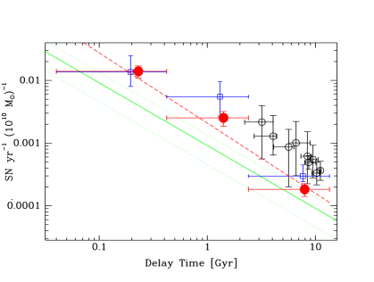
Figure 1: Recovered SN Ia DTD for the SDSS2 SN sample. Filled red circles mark the best-fit DTD values for each time bin, whose time range is indicated by the horizontal error bars. Vertical error bars show the Gaussian $1\sigma$ uncertainties. Red dashed line is the best power-law fit, with index $-1.12$, to the recovered DTD. Previous DTD measurements also shown are: M11 analysis of the nearby LOSS sample (empty blue squares, with central values slightly shifted to the left, for clarity); Maoz et al. (2010) analysis based on SN Ia rates in galaxy clusters (empty black circles); and $t^{-1}$ power law DTD found by Graur et al. (2011), based on comparison of volumetric SN Ia rates and cosmic SFH (solid green line, with dotted lines marking the $1\sigma$ range).

Also shown in Fig. 1, for comparison, are a number of other recent DTD estimates. The value we find for the prompt DTD component, $\Psi_{1}$, is in excellent agreement with the one found in M11. The values of the intermediate and delayed components, $\Psi_{2}$ and $\Psi_{3}$, respectively, are a factor $\sim 2$ lower than found by M11. In the case of $\Psi_{2}$, the difference is not statistically significant, and furthermore the M11 value may have been overestimated due to some residual “leak” of signal from $\Psi_{1}$ (see M11, and below). The difference in $\Psi_{3}$ values between M11 and the present work, however, is more significant, at the $\sim 2\sigma$ level. Furthermore, both the current and the M11 $\Psi_{3}$ measurements are lower than the DTD values implied by a number of independent measurements of SN Ia rates in galaxy clusters, as compiled in Maoz et al. (2010), and also shown in Fig. 1. On the other hand, as also shown in the figure, our new $\Psi_{3}$ measurement is consistent in level with the DTD level at long delays found by Graur et al. (2011) from comparison of volumetric SN Ia rates to cosmic SFH. Our result thus revives previous speculation that the SN Ia rate in old populations may be enhanced by a factor of a few in cluster environments, compared to field environments (Sharon et al. 2007; Mannucci et al. 2008). The intermediate $\Psi_{3}$ value found in M11 could be due to a relatively large fraction of LOSS galaxies in clusters. Among all the LOSS galaxies, 20% are in galaxy clusters that are listed in the NED database, based on the same criteria as applied in Mannucci et al. (2008; projected separation $<1.5$ Mpc, redshift difference $<1000$ km s^-1). The fraction of the early-type LOSS galaxies in clusters will be higher. Assuming the SDSS2 galaxy sample, in contrast, is dominated by a field population, a factor-few enhancement of the SN Ia rate in clusters could lead to the higher $\Psi_{3}$ value measured in M11, compared to here. We defer to future work a more detailed examination of this possibility regarding the LOSS sample.

It is important to note that the errors shown in Fig. 1 are statistical only. A systematic source of error, one that is difficult to estimate, is associated with the SFH reconstruction of each galaxy (see Tojeiro et al. 2009, M11, and Section 4.3, below).

Table 2: Recovered Delay Time Distribution

Sample	$N_{\rm gal}$	$N_{\rm SN}$	$\Psi_{1}$	$\Psi_{2}$	$\Psi_{3}$	$N_{\rm SN}/M$
			0–0.42 Gyr	0.42–2.4 Gyr	2.4–14 Gyr
(1)	(2)	(3)	(4)	(5)	(6)	(7)
Full	66,000	132	$140\pm 30$	$25.1\pm 6.3$	$1.83\pm 0.42$	$0.00130\pm 0.00015$
High $s$	66,000	67	$87\pm 24$	$10.5\pm 4.2$	$0.78\pm 0.32$	$0.00066\pm 0.00011$
Low $s$	66,000	45	$24\pm 15$	$5.7\pm 3.6$	$0.96\pm 0.27$	$0.00032\pm 0.00007$

Column header explanations:

(1)- Sample used to derive DTD: Full sample, high-stretch sample, or low-stretch sample.

(2) - Number of galaxies in sample.

(3) - Number of SNe in sample.

(4-6) - DTD rates and 68% uncertainty ranges, in units of $10^{-14}$ SNe yr${}^{-1}\,{\rm M}_{\odot}^{-1}$.

(7) - Time-integrated DTD, in units of SNe ${\rm M}_{\odot}^{-1}$.

We have used $\chi^{2}$ minimization to fit model power-law functions, $\Psi(t)\propto t^{\beta}$, to the recovered binned DTD, with the amplitude and the power-law index as free parameters. The model is averaged over each time bin, to obtain the value that is compared to the observed DTD value for that bin. The best-fitting power-law has an index of $\beta=-1.12\pm 0.08$. Our result augments a growing number of indications for a DTD that is a power law with a slope of $\sim-1$. However, Fig. 1 suggests that a better description may be a function that steepens somewhat at long delays, compared to a single power law. Further studying the DTD at such a level of detail will require better temporal resolution. The present three-bin time resolution is dictated by the spectral resolution and the signal-to-noise ratio of the SDSS spectra.

4.2 SN Ia production efficiency

As discussed in Maoz & Mannuci (2012), and references therein, another interesting observable is the DTD normalization. It can be discussed in the context of the integral of the DTD over the age of the universe, $t_{0}$,

$$N_{\rm SN}/M=\int_{0}^{t_{0}}\Psi(t)~{}dt,$$ (9)

which gives the total number of SNe that eventually explode, per unit stellar mass formed in a short burst of star formation. The integral in Eq. 9 can be approximated by a sum over the binned DTD,

$$N_{\rm SN}/M\approx\sum_{j=1,K}\Psi_{j}\Delta t_{j}.$$ (10)

From the simulations described in M11, for declining power-law DTDs represented with three time bins, Eq. 10 typically underestimates $N_{\rm SN}/M$ systematically by $\sim 10-20\%$.

For the SDSS2 sample, we obtain $N_{\rm Ia}/M=0.00130\pm 0.00015~{}{\rm M}_{\odot}^{-1}$. This is lower than the $N_{\rm Ia}/M=0.0020\pm 0.0006~{}{\rm M}_{\odot}^{-1}$ found in M11 for the LOSS sample, although consistent with it, given the larger uncertainty of the M11 result. The present result is also consistent with a lower estimate of $N_{\rm Ia}/M=0.0010\pm 0.0005~{}{\rm M}_{\odot}^{-1}$ found by Graur et al. (2011), from comparison of volumetric SN Ia rate evolution and cosmic SFH. A very recent analysis of the volumetric rates by Perrett et al. (2012) gives $N_{\rm Ia}/M\sim 0.0006-0.0010~{}{\rm M}_{\odot}^{-1}$ (after converting their result to a diet-Salpeter IMF), similar to the Graur et al. (2011) result. As was the case when considering the DTD amplitude $\Psi_{3}$, above, the estimates of $N_{\rm Ia}/M$ from galaxy clusters are higher when based on cluster SN Ia rates vs. redshift, and even more so when based on cluster iron mass content (Maoz et al. 2010; see Maoz & Mannucci 2012, table 1). For example, the $2\sigma$ lower limit is $N_{\rm Ia}/M>0.0017~{}{\rm M}_{\odot}^{-1}$ from SN Ia rates in clusters, and $N_{\rm Ia}/M>0.0034~{}{\rm M}_{\odot}^{-1}$ from the iron mass content. It remains to be seen whether this is the result of some systematic error, or a real enhancement of SN Ia production in cluster environments (Sharon et al. 2007; Mannucci et al. 2008; Sand et al. 2011).

The SN Ia number per formed stellar mass, $N_{\rm Ia}/M$, can easily be related to the fraction, $\eta$, of stars in some initial mass range $[m_{1},m_{2}]$, that eventually explode as SNe Ia:

$$\eta=\frac{N_{\rm Ia}}{M}\frac{\int_{0.1}^{100}m(dN/dm)dm}{\int_{m_{1}}^{m_{2}}(dN/dm)dm},$$ (11)

where $dN/dm$ is the IMF. For the “diet Salpeter” IMF (which, again, gives results similar to the Kroupa IMF assumed by the VESPA SFH reconstruction), and an initial mass range of 3–8 M_⊙, often considered for the primary stars of SN Ia progenitor systems, the ratio of the two integrals equals 33. Our present result of $N_{\rm Ia}/M=0.00130\pm 0.00015~{}{\rm M}_{\odot}^{-1}$ translates to $\eta=4.3\pm 0.5$%. Interestingly, Mannucci et al. (2006) estimated $\eta=4.3\%$ by modeling SN Ia rates per unit mass as a function of galaxy colors in a local sample.

4.3 Analysis of cross-talk between bins

In the M11 analysis of the LOSS SN sample and the VESPA SFHs of the monitored LOSS galaxies, a major systematic error emerged, due to the limited $3^{\prime\prime}$ aperture size of the SDSS fibres. The LOSS galaxies are relatively nearby, $z<0.05$, with half of them at $z<0.022$, and are hence large in angle. The SDSS spectra in many cases are therefore dominated by old populations in the centres of the galaxies probed by the fibres. However, many of the LOSS SNe exploded in the outer regions, where there is ongoing star formation outside the aperture of the SDSS spectroscopy. As a result, the DTD solution mistakenly associated these SNe with an old population, and hence a large delay. The result was an artificially enhanced DTD amplitude in the intermediate and delayed bins, at the expense of the prompt bin, an effect referred to as DTD inter-bin “leak” or “cross-talk” in M11. To mitigate this effect, M11 defined a culled sample of galaxies that excluded Sab-Sbc Hubble types, which are most susceptible to this stellar-population misrepresentation by the fibre spectrum. The DTD derived from the culled galaxy sample, and the SNe that they hosted, had a much-reduced DTD leak, but at the price of a reduced sample of SNe, resulting in larger DTD Poisson errors.

The DTD inter-bin leak, and its reduction in the culled sample, was diagnosed in M11 by deriving the DTD for core-collapse (CC) SNe. Core-collapse SNe explode within $\lesssim 40$ Myr of star formation. The CC SN DTD should have zero amplitude on timescales much longer than this, particularly in the bins at $t>420$ Myr. Thus, any signal in those bins is due to a leak. Compared to LOSS, we expect the SDSS2 sample to have smaller or no inter-bin DTD leaks. The typical redshift of the SN hosts is $z=0.15$, an order of magnitude larger than for LOSS, and all but three of the SDSS2 SN hosts are at $z>0.05$. The spectra from the SDSS fibres should thus represent well the entire stellar population of each galaxy. To verify this, we have compiled a sample of all SNe in the SDSS2 website’s list that have been spectroscopically classified as CC SNe and are associated with a Stripe 82 galaxy with a VESPA SFH. There are 41 such CC SNe. This list is, of course, far from complete, particularly because the main SDSS2 science objective was the discovery of SNe Ia, and events suspected to be CC SNe had low priority for spectroscopic followup (D10). Nevertheless, even in a small and incomplete sample, DTD leak will still manifest itself in the form of a DTD signal at long delays.

The leak effect can be quantified via the ratio between the intermediate and the prompt CC-SN DTD components, $\Psi_{2}/\Psi_{1}$, which should be zero when there is no leak of signal from the first to the second DTD bin. In the full LOSS CC sample of M11 (see their table 1), $\Psi_{2}/\Psi_{1}=0.165\pm 0.045$, i.e., there is clear presence of a leak. In the M11 subsample that was culled of Sab-Sbc Hubble types, this ratio was reduced to $\Psi_{2}/\Psi_{1}=0.077\pm 0.050$, which is consistent with zero. For the SDSS2 CC-SN sample, we find $\Psi_{2}/\Psi_{1}=0.069\pm 0.050$, similar to the ratio in the culled LOSS sample, and again consistent with zero.

As another test of cross-talk, we have recalculated the SN Ia DTD, limiting the galaxies and the SNe to be above some redshift threshold. Since the fibre-related DTD leak decreases with increasing galaxy redshift (as more of the galaxy’s extent is included in the aperture), we expect a change in the DTD when changing thresholds, as was indeed seen in M11. In the SDSS2 sample, however, we see no significant changes in the SN Ia DTD when limiting the sample to higher redshifts. We conclude that the SDSS2 sample’s DTD is largely free of the inter-bin cross talk due to the SDSS fibre aperture.

4.4 Stretch-dependent DTD

Most DTD recovery work to date has considered only a univariate, universal, DTD. A correlation has been known for some time (e.g. Hamuy et al. 2000; Neill et al. 2009; Hicken et al. 2009) between the age of a SN Ia host and the SN luminosity (or, equivalently, its light curve’s “stretch parameter”, $s$, or the mass of radioactive Ni synthesized). Old galaxies tend to host low-luminosity SNe Ia, while star-forming galaxies tend to have luminous SNe Ia. This is an observed link between the progenitor population and the energy of the explosion, and thus may provide a critical clue to the progenitor question. However, it is only through the DTD recovery approach that one can distill this link from the data, decoupled from the SFHs of the individual galaxies. B10 used the stretches of their SN Ia sample’s light curves to divide their sample into high-stretch and low-stretch subsamples, and derived the DTD for each subsample. This was the first derivation of a bivariate $\Psi(t,s)$ distribution, one with three delay-time bins and two stretch bins. Here, “DTD” is no longer an appropriate name, as this is now the bivariate distribution (or “response function”) of delay times and stretches. The bivariate response contains information that is additional to the distribution’s univariate projection, the DTD, as it gives not only the age of the progenitor systems but also the run of explosion energies for each progenitor age. B10 indeed found that luminous, high-stretch, SNe Ia tend to have most of their DTD power at short delays, while low-stretch, underluminous, SNe Ia have a DTD that peaks in the longest-delay bin.

To test this result with our newly defined SDSS2 sample and analysis, we have created low-stretch and high-stretch SN Ia subsamples, adopting, like B10, a border between the two populations of $s=0.92$. Among the 61 of our SNe that are from the D10 sample with spectroscopic confirmation, 50 are in the B10 sample, and we adopt the B10 classifications for these SNe as high- or low-stretch. We exclude the remaining 11 D10 SNe from the present analysis. For the 62 photometrically classified SNe Ia that are from S11, we convert the $\Delta M_{15}$ values, tabulated by S11, to stretch, $s$, using (Guy et al. 2005, their footnote 7),

$$s=-0.59~{}\Delta M_{15}+1.55.$$ (12)

The 9 additional SNe from our full sample, that were photometrically classified by D10, do not have stretch, or analogous, parameters tabulated, so we also exclude them from the present analysis. With this selection, we obtain 45 low-stretch SNe Ia and 67 high-stretch SNe.

Table 2 lists the DTDs we obtain separately for the low-stretch and high-stretch subsamples. The high-stretch DTD has a $3.5\sigma$ signal in the prompt time bin, and $\sim 2.5\sigma$ detections in the later time bins. The best-fitting power law to this DTD has an index $-1.12\pm 0.13$. The low-stretch DTD has only $1.5\sigma$ detections in the prompt and intermediate time bins. Those DTD components are thus consistent with zero, but higher $\Psi_{1}$ and $\Psi_{2}$ values, giving similar component ratios as in the high-stretch DTD, also cannot be ruled out. The delayed low-stretch component, $\Psi_{3}$, does have a $>3\sigma$ signal. A power-law index in this case is $-0.9^{+0.3}_{-0.15}$.

Qualitatively, these results are similar to those of B10, in the sense that the high-stretch SNe have a DTD with a strong prompt signal, while the low-stretch SNe have a strong signal in the delayed bin. However, the present analysis does not reproduce the nearly one-to-one correspondence reported by B10, where essentially all high-stretch SNe derive from a young population, and all low-stretch SNe from an old one (see also further discussion of the B10 results in Section 4.5, below). Rather, in the present analysis, there may be a trend in the above sense, but high-stretch SNe do have significant non-zero amplitudes in their intermediate and delayed DTD bins. And, within the current uncertainties, low-stretch SNe may have non-zero prompt and intermediate-delay DTD components.

We suspect that the difference between the present results and those of B10 may be due to selection effects that arise from the use, by B10, of a sample that includes only spectroscopically confirmed SNe Ia. The SDSS2 survey was strongly oriented toward dicovering SNe Ia for cosmographic purposes. The selection of candidates for spectroscopic followup, and the success of those followup observations, were both likely tied to the luminosity of the SN (and hence to its stretch) and to the type of host galaxy. For example, a candidate in an early-type galaxy would have been likely considered a promising SN Ia, even if its luminosity was not high. Its spectroscopy may have been more likely to succceed in the presence of the lower host starlight background, compared to a similar low-luminosity candidate in a star-forming galaxy. Such biases could artificially eliminate, in the spectroscopically confirmed sample, low-luminosity SNe Ia in star-forming galaxies, and this would reduce or eliminate the $\Psi_{1}$ component in the low-stretch sample. The more-complete, spectroscopic plus photometric, sample analyzed here is more immune to such a possible selection effect, and may thus be reflecting better the true DTDs. Recently, Perrett et al. (2012) have also failed to find strong differences in volumetric rate evolution between low-$s$ and high-$s$ SNe Ia. Larger, well-defined, samples will be able to further probe the bivariate distribution of SN Ia delay and stretch.

There is some concern that the DTD that we have recovered may be biased, due to the known correlation between host galaxy age, or star-formation rate, on the one hand, and SN stretch or luminosity, on the other. The D10 detection efficiency function that we have used does not account for this correlation. Thus, for example, early-type galaxies, which tend to host lower-luminosity SNe, would have a true detection efficiency lower than that of D10. Our overestimate of the efficiency could then lead to a perceived paucity of SNe Ia in old populations, and hence to an underestimate of the true $\Psi_{3}$ DTD component. To gauge the possible magnitude of such an effect, we have repeated the DTD derivation, but modifying the D10 detection efficiency function as follows. Sullivan et al. (2006) have shown (their fig. 11) that galaxies with specific star-formation rates ${\rm sSFR}>10^{-9.5}{\rm yr}^{-1}$ host SNe with a mean stretch of $s\approx 1.03$, while the most passive galaxies, with ${\rm sSFR}<10^{-12}{\rm yr}^{-1}$ have SNe with mean $s\approx 0.87$. This change in $s$ corresponds to a change in SN peak absolute magnitude by about 0.25 mag. Such a change in brightness, in turn, corresponds to a change in redshift of $\Delta z/z=\pm 6\%$. For galaxies that, based on their VESPA SFHs, have current specific star-formation rates ${\rm sSFR}>10^{-9.5}{\rm yr}^{-1}$, we therefore modify the D10 efficiency function (described in Section 2.1), such that it declines linearly from $z=0.184$ (rather than $z=0.175$), reaching zero at $z=0.42$ (rather than $z=0.4$). For the passive galaxies with ${\rm sSFR}<10^{-12}{\rm yr}^{-1}$, we assume a detection function that declines linearly from $z=0.166$, reaching zero already at $z=0.38$. For the intermediate, weakly star-forming galaxies, we use the D10 detection efficiency, as before. We find that the recovered DTD is only slightly affected by this modification of the detection efficiency, with $\Psi_{1}$ decreasing by 10% and $\Psi_{3}$ increasing by 10%. The change leads to a slightly less steep power-law fit to the DTD, with an index of $\beta=-1.07\pm 0.07$.

4.5 Comparison of the B10 and M11 DTD recovery methods

As elaborated above, the SN Ia sample and the details of the DTD calculation based on SDSS2 SNe differ in a number of ways between the present work and that of B10. Nevertheless, it is interesting to compare the performance and results of the two different algorithmic approaches – on the one hand, that of M11 and of this work, i.e., comparing observed and predicted (given a DTD model) SN numbers in each galaxy; and on the other hand that of B10, comparing the observed mean host spectrum to a mock mean host spectrum (for a given DTD model). We have therefore calculated a DTD reconstruction with the M11 approach, but reproducing as closely as possible the SN Ia sample and the assumptions of B10.

To construct a SN Ia sample analogous to the one of B10, we have matched coordinates and redshifts between the 101 SNe Ia in table 2 of B10 and the current Stripe 82 VESPA sample of galaxies (without any RA limits). We have matched 89 of the B10 SNe to host galaxies (we note that 37 of the SNe in B10 have mis-typed declination signs – positive instead of negative). This smaller number of SNe, 89 compared to 101, is expected, given our smaller galaxy sample (66,000) compared to that of B10 (77,000). Among these 89 SNe Ia, B10 listed 32 as low-stretch and 57 as high-stretch. We have then run these low-stretch and high-stretch samples through the M11 DTD recovery algorithm, but using the same efficiency function assumed by B10, with the same parameters that they assumed for high-stretch and low-stretch SNe. In this calculation, we do not correct for cosmological time dilation, and do not scale down the VESPA masses by 0.55 (see §2, above). We find for the three of components of the DTD, $\Psi_{1}$, $\Psi_{2}$, and $\Psi_{3}$, respectively, in units of $10^{-14}$ yr^-1M${}_{\odot}^{-1}$,
Low-stretch: ($0\pm 28;~{}~{}~{}0\pm 5;~{}~{}~{}1.3\pm 0.4$);
High-stretch: ($65\pm 15;~{}~{}~{}8\pm 3;~{}~{}~{}0.1\pm 0.2$).
Table 3 and figure 7 of B10 give, for several of the low-stretch and high-stretch $\Psi$ components ($\epsilon_{h,2}$, and $\epsilon_{l,2}$, in their nomenclature) their results and uncertainties. To these uncertainties we have added $1\sigma$ Poisson errors, not included in B10. The B10 $\Psi_{i}$ results are,
Low-stretch: ($0\pm 20;~{}~{}~{}0\pm 5;~{}~{}~{}1.6\pm 0.3$);
High-stretch: ($75\pm 19;~{}~{}~{}8\pm 5;~{}~{}~{}0.3\pm 0.2$).
We see that the best-fit results and the uncertainties found by the two algorithms are quite similar. The slightly higher values found by B10 for the significantly non-zero components may be due to the fact that B10 draw the DTD values that they test from an assumed prior distribution, while in M11 and here we do an adaptive grid search for the best fitting DTD in the 3D space of $\Psi_{1}$, $\Psi_{2}$, and $\Psi_{3}$.

5 Discussion and summary

We have taken the DTD recovery method presented in M11, where it was applied to the LOSS SN sample, and applied it here to a subsample of SDSS2 SNe Ia that were hosted by Stripe-82 SDSS galaxies with VESPA SFH reconstructions. Among all of the DTD recontructions to date that are based on detailed SFHs of individual galaxies (B10; M11; Maoz & Badenes 2010; this work), we have obtained the DTD that is the most precise (in terms of Poisson errors) and the most accurate (in terms of control of systematic errors). The full M11 sample was systematically affected by the limited SDSS fibre aperture, which led to cross talk between DTD bins. In the reduced M11 sample, where this problem was mitigated, only 49 SNe Ia remained, leading to large Poisson errors. In the analysis by Maoz & Badenes (2010) of 77 Magellanic Cloud SN remnants, the bulk of the DTD signal was at $t<35$ Myr, corresponding to core-collapse SNe. This meant that only of order 10 SNe Ia were effectively driving the SN Ia DTD, which was therefore very noisy. Another possible systematic error in Maoz & Badenes (2010) was contamination of the SNa Ia DTD by CC SNe, with progenitors near the poorly known progenitor age border between CC-SNe and WD formation.

The SNe from SDSS2, which are at larger distances and are well classified, can avoid the above systematics, and at the same time allow for relatively large numbers of SNe Ia. The B10 analysis of SDSS2 SNe, however, used a limited sample, available at the time, consisting only of spectrally confirmed SNe. Furthermore, B10 estimated a detection efficiency function that did not take into account the details of the real observing patterns, the detection process, classification, and sample selection, details that were later quantified by D10, based on real-time detection simulations. Finally, the B10 analysis omitted necessary corrections to the SN visibility times and to the stellar masses of the galaxies. All of the above are potential sources of systematic error, affecting each DTD component by up to a factor $\sim 2$. In our renewed definition and analysis of an SDSS2 SN sample, we have addressed these issues. In this analysis, we have detected for the first time, at a highly significant level, an intermediate-delay DTD component, at $0.42<t<2.4$ Gyr. B10 and M11 observed such a component only at the $\sim 2\sigma$ level. In addition, the completeness of the sample and the consideration of absolute stellar mass, visibility time, and efficiency, permit a robust derivation of absolute DTD levels.

It is interesting to consider the cause behind the much more significant detection of an intermediate-delay DTD component, $\Psi_{2}$, compared to the B10 analysis of a differently defined SDSS2 SN Ia sample. Given that the M11 and B10 algorithms give similar results and uncertainties (Section 4.5, above), the difference in the $\Psi_{2}$ significance could be due to the differences in the SN samples, the differences in the adopted efficiency functions, or both. To investigate this, we have recovered best-fit DTDs with the present SN Ia sample (Table 1), but using the B10 efficiency function, and omitting other corrections, as in Section 4.5. Alternatively, we have used the B10 SN sample as described in Section 4.5, but using the empirical D10 efficiency function, $1+z$ correction, and so on, as in our main calculation. We find that neither choice, alone, raises much the $\Psi_{2}$ detection significance. Apparently, the improvement results from the combination of a carefully selected, relatively complete, sample of SNe, and a realistic efficiency function, one that embodies the selection effects of that same SN sample. The two, together, sharpen the correlation between the presence of SNe Ia and an intermediate-age stellar population in some galaxies, and thus reveal clearly the $\Psi_{2}$ component.

Our findings point to a continuous distribution of SN Ia delay times. Although recent observational developments have led to discussions of “prompt and delayed SNe Ia”, “two SN Ia channels/populations”, “a bimodal DTD”, and so on, theoretical binary population synthesis models have almost always predicted a broad and continuous DTD, even for a single physical channel (e.g. DD). Thus, the continuous observational DTDs that are emerging (Totani et al. 2008; Maoz et al. 2010; this work) are not unexpected. Naturally, DTDs recovered in the future with finer time resolution may still reveal a real bimodality. The current coarse time resolution of the DTD is dictated by the resolution of the galaxy SFHs. Future improved data will also permit recovery of a better-resolved, and higher signal-to-noise, bivariate distribution of delay and stretch, $\Psi(t,s)$, that could sharpen the current hints of a relation between the progenitor age and the explosion energy.

As in most of the recent studies, the DTD we find appears to be consistent with the $\sim t^{-1}$ form generally expected in the DD scenario. This result joins others that are strongly suggestive of DD progenitors for at least some SNe Ia. Most notable among these are the absence of any signs of the putative donor star, a few years before, and during the explosion of SN2011fe (Li et al. 2011c, Nugent et al. 2011, Horesh et al. 2012), and 400 years after the explosion that left the SN remnant 0509$-$67.5 (Schaefer & Pagnotta 2012). It is noteworthy that the main objection to the DD model has been theoretical, arguing that a DD merger cannot produce an event with the characteristics of SNe Ia. The fact that there are, by now, a couple of cases where we may have witnessed DD mergers producing normal SNe Ia suggests that the theoretical objection could be somehow flawed (unless the absence of a companion, in these cases, is the result of one of the “SN on hold” scenarios mentioned in Section 1, assuming they work). If indeed the DD scenario is physically possible after all, perhaps most or even all SNe Ia could result from DD mergers. Examining the evidence from the opposite direction, Maoz et al. (2012) and Badenes & Maoz (2012) have recently estimated the specific merger rate of Galactic WD binaries. They found that, if one considers all WD mergers, most of which have sub-Chandrasekhar merged masses, but only a few tenths of a solar mass below this limit, their merger rate is remarkably similar to the specific SN Ia rate of Milky-Way-like galaxies. Naturally, this coincidence is meaningful only if sub-Chandrasekhar CO-CO WD mergers can indeed produce a SN Ia, which is still an open question (e.g. van Kerkwijk et al. 2010; Guillochon et al. 2010; Pakmor et al. 2011).

Another interesting result of our analysis is the absolute DTD normalization that we find – lower than most of the recent determinations based on SN Ia rates in nearby galaxies and in galaxy clusters, but consistent with the levels found based on volumetric SN Ia rates. This result relaxes some of the tension between the previous, high, observational SN Ia production efficiencies, and the lower predictions from binary population synthesis models (see, e.g. Maoz 2008; Mennekens et al. 2010). On the other hand, our result re-floats the possibility that SNe Ia, for some reason, are produced more efficiently in galaxy cluster environments than in field environments. If this is true, it could be the result of an IMF that depends on environment. Evidence has accumulated recently that the most massive elliptical galaxies have “bottom-heavy” IMFs, with low-mass components as steep, or even steeper than, the Salpeter IMF (e.g. Treu et al. 2010; Cappellari et al. 2012; Conroy & van Dokkum 2012). Clusters host the most massive ellipticals. Thompson (2011) has proposed that a large fraction of SN Ia progenitor systems are triples, in which a low-mass tertiary induces ellipticity in the inner WD binary via the Kozai (1962) mechanism, significantly increasing the time-integrated number of DD systems that merge (and presumably produce SNe Ia). A speculative possibility that we raise is that, in cluster galaxies, the large availability of low-mass stars translates into more tertiaries, and hence a larger SN Ia production efficiency.

To summarize, we have constructed a new SDSS2 SN Ia sample that is more complete and has a better-characterized detection efficiency than what was available in B10. We have analyzed it with the methodology of M11, but avoiding the small sample size and the systematic errors in SFH that were unavoidable in the LOSS sample of M11, while making several necessary corrections that were omitted in B10. In the end, we find a SN Ia DTD that is more accurate and more precise than the ones found by either B10 and M11. For the first time, a DTD based on the three time bins used here shows a highly significant signal in all three bins. The DTD is consistent in form with the $t^{-1}$ found in the studies reviewed above (including B10 and M11), but differs in absolute normalization from some of those studies.

The SN Ia progenitor problem is far from solved. However, our results demonstrate how our view of the SN Ia DTD can progressively improve by means of analysis of samples of SNe that are progressively larger, purer, more complete, and well-characterized, and with samples of monitored galaxies with SFHs that are better determined, systematically, temporally, and spatially. These improved views will continue to play a role in resolving the progenitor issue.

References

- [1] Adelman-McCarthy, J.K. et al. 2008, ApJS, 175, 297
- [Badenes et al.(2010)] Badenes, C., Maoz, D., & Draine, B. T. 2010, MNRAS, 407, 1301
- [Badenes & Maoz(2012)] Badenes, C., & Maoz, D. 2012, ApJ, 749, L11
- [Bell et al.(2003)] Bell, E. F., McIntosh, D. H., Katz, N., & Weinberg, M. D. 2003, ApJS, 149, 289
- [Bloom et al.(2012)] Bloom, J. S., Kasen, D., Shen, K. J., et al. 2012, ApJ, 744, L17
- [Blanton et al.(2001)] Blanton, M. R., Dalcanton, J., Eisenstein, D., et al. 2001, AJ, 121, 2358
- [Brandt et al.(2010)] Brandt, T. D., Tojeiro, R., Aubourg, É., Heavens, A., Jimenez, R., & Strauss, M. A. 2010, AJ, 140, 804 (B10)
- [Brown et al.(2012)] Brown, P. J., Dawson, K. S., Harris, D. W., et al. 2012, ApJ, 749, 18
- [Cappellari et al.(2012)] Cappellari, M., McDermid, R. M., Alatalo, K., et al. 2012, Nature, 484, 485
- [Cash(1979)] Cash, W. 1979, ApJ, 228, 939
- [] Chomiuk, L., Soderberg, A.M., Moe, M., et al. 2012, ApJ, 750, 164
- [] Conroy, C., & van Dokkum, P. 2012, arxiv:1205.6473
- [Dilday et al.(2008)Dilday, Kessler, Frieman, Holtzman, Marriner, Miknaitis, Nichol, Romani, Sako, Bassett, Becker, Cinabro, DeJongh, Depoy, Doi, Garnavich, Hogan, Jha, Konishi, Lampeitl, Marshall, McGinnis, Prieto, Riess, Richmond, Schneider, Smith, Takanashi, Tokita, van der Heyden, Yasuda, Zheng, Barentine, Brewington, Choi, Crotts, Dembicky, Harvanek, Im, Ketzeback, Kleinman, Krzesiński, Long, Malanushenko, Malanushenko, McMillan, Nitta, Pan, Saurage, Snedden, Watters, Wheeler, & York] Dilday B., Kesslesr, R., Frieman, J., et al., 2008, ApJ, 682, 262
- [Dilday et al.(2010a)Dilday, Smith, Bassett, Becker, Bender, Castander, Cinabro, Filippenko, Frieman, Galbany, Garnavich, Goobar, Hopp, Ihara, Jha, Kessler, Lampeitl, Marriner, Miquel, Mollá, Nichol, Nordin, Riess, Sako, Schneider, Sollerman, Wheeler, Östman, Bizyaev, Brewington, Malanushenko, Malanushenko, Oravetz, Pan, Simmons, & Snedden] Dilday B., Smith, M., Bassett, B., et al., 2010, ApJ, 713, 1026 (D10)
- [Dilday et al.(2012)] Dilday, B., Howell, D. A., Cenko, S. B., et al. 2012, arXiv:1207.1306
- [Di Stefano et al.(2011)] Di Stefano, R., Voss, R., & Claeys, J. S. W. 2011, ApJ, 738, L1
- [Frieman et al.(2008)] Frieman, J. A., Bassett, B., Becker, A., et al. 2008, AJ, 135, 338
- [Guillochon et al.(2010)] Guillochon, J., Dan, M., Ramirez-Ruiz, E., & Rosswog, S. 2010, ApJ, 709, L64
- [Graur et al.(2011)] Graur, O., Poznanski, D., Maoz, D., et al. 2011, MNRAS, 417, 916
- [Guy et al.(2005)] Guy, J., Astier, P., Nobili, S., Regnault, N., & Pain, R. 2005, A&A, 443, 781
- [Harris & Zaritsky(2004)] Harris, J., Zaritsky, D. 2004, ApJ, 604, 167
- [Harris & Zaritsky(2009)] Harris, J., Zaritsky, D. 2009, AJ, 138, 1243
- [2] Hamuy, M., Trager, S.C., Pinto, P.A., Phillips, M.M., Scummer, R.A., Ivanov, V., Suntzeff, N.B. 2000, AJ, 120, 1479
- [Han & Podsiadlowski(2004)] Han, Z., & Podsiadlowski, P. 2004, MNRAS, 350, 1301
- [Hicken et al.(2009)] Hicken, M., Wood-Vasey, W. M., Blondin, S., et al. 2009, ApJ, 700, 1097
- [Horesh et al.(2011)] Horesh, A., Kulkarni, S. R., Fox, D. B., et al. 2012, ApJ, 746, 21
- [Howell(2011)] Howell, D. A. 2011, Nature Communications, 2, 350
- [Iben & Tutukov(1984)] Iben, I., Jr., & Tutukov, A. V. 1984, ApJS, 54, 335
- [Ilkov & Soker(2012)] Ilkov, M., & Soker, N. 2012, MNRAS, 419, 1695
- [Jha et al.(2007)] Jha, S., Riess, A. G., & Kirshner, R. P. 2007, ApJ, 659, 122
- [Justham(2011)] Justham, S. 2011, ApJ, 730, L3
- [Kasen(2010)] Kasen, D. 2010, ApJ, 708, 1025
- [Kashi & Soker(2011)] Kashi, A., & Soker, N. 2011, MNRAS, 417, 1466
- [Kozai(1962)] Kozai, Y. 1962, AJ, 67, 591
- [Kroupa(2007)] Kroupa, P. 2007, arXiv:astro-ph/0703124
- [Leaman et al.(2011)] Leaman, J., Li, W., Chornock, R., & Filippenko, A. V. 2011, MNRAS, 412, 1419
- [Li et al.(2011)] Li, W., et al. 2011a, MNRAS, 412, 1441
- [Li et al.(2011)] Li, W., Chornock, R., Leaman, J., Filippenko, A. V., Poznanski, D., Wang, X., Ganeshalingam, M., & Mannucci, F. 2011b, MNRAS, 412, 1473
- [Li et al.(2011)] Li, W., Bloom, J. S., Podsiadlowski, P., et al. 2011c, Nature, 480, 348
- [Mannucci et al.(2005)] Mannucci, F., Della Valle, M., Panagia, N., Cappellaro, E., Cresci, G., Maiolino, R., Petrosian, A., & Turatto, M. 2005, A&A, 433, 807
- [Mannucci et al.(2006)] Mannucci, F., Della Valle, M., & Panagia, N. 2006, MNRAS, 370, 773
- [Mannucci et al.(2008)] Mannucci, F., Maoz, D., Sharon, K., Botticella, M. T., Della Valle, M., Gal-Yam, A., & Panagia, N. 2008, MNRAS, 383, 1121
- [Maoz(2008)] Maoz, D. 2008, MNRAS, 384, 267
- [Maoz et al.(2010)] Maoz, D., Sharon, K., & Gal-Yam, A. 2010, ApJ, 722, 1879
- [Maoz & Badenes(2010)] Maoz, D., & Badenes, C. 2010, MNRAS, 407, 1314
- [Maoz et al.(2011)] Maoz, D., Mannucci, F., Li, W., Filippenko, A. V., Della Valle, M., & Panagia, N. 2011, MNRAS, 412, 1508 (M11)
- [Maoz et al.(2012)] Maoz, D., Badenes, C., & Bickerton, S. J. 2012, ApJ, 751, 143
- [Maoz & Mannucci(2012)] Maoz, D., & Mannucci, F. 2012, PASA, in press, arXiv:1111.4492
- [Maraston(2005)] Maraston, C. 2005, MNRAS, 362, 799
- [Meng et al.(2011)] Meng, X. C., Chen, W. C., Yang, W. M., & Li, Z. M. 2011, A&A, 525, A129
- [Mennekens et al.(2010)] Mennekens, N., Vanbeveren, D., De Greve, J. P., & De Donder, E. 2010, A&A, 515, A89
- [Neill et al.(2009)] Neill, J. D., et al. 2009, ApJ, 707, 1449
- [Nelemans et al.(2001)] Nelemans, G., Yungelson, L. R., Portegies Zwart, S. F., & Verbunt, F. 2001, A&A, 365, 491
- [Nomoto(1982)] Nomoto, K. 1982, ApJ, 253, 798
- [Nomoto & Iben(1985)] Nomoto, K., & Iben, I., Jr. 1985, ApJ, 297, 531
- [] Nugent, P., et al. 2011, Nature, 480, 344
- [Pakmor et al.(2010)] Pakmor, R., Kromer, M., Röpke, F. K., Sim, S. A., Ruiter, A. J., & Hillebrandt, W. 2010, Nature, 463, 61
- [Pakmor et al.(2011)] Pakmor, R., Hachinger, S., Röpke, F. K., &; Hillebrandt, W. 2011, A&A, 528, A117
- [Patat et al.(2007)] Patat, F., et al. 2007, Science, 317, 924
- [Perrett et al.(2012)] Perrett, K., Sullivan, M., Conley, A., et al. 2012, arXiv:1206.0665
- [Press et al.(1992)] Press, W. H., Teukolsky, S. A., Vetterling, W. T., & Flannery, B. P. 1992, Cambridge: University Press, —c1992, 2nd ed.,
- [Rest et al.(2008)] Rest, A., Matheson, T., Blondin, S., et al. 2008, ApJ, 680, 1137
- [Ruiter et al.(2011)] Ruiter, A. J., Belczynski, K., Sim, S. A., Hillebrandt, W., Fryer, C. L., Fink, M., & Kromer, M. 2011, MNRAS, 417, 408
- [Sako et al.(2008)] Sako, M., Bassett, B., Becker, A., et al. 2008, AJ, 135, 348
- [Sako et al.(2011)] Sako, M., Bassett, B., Connolly, B., et al. 2011, ApJ, 738, 162 (S11)
- [Sand et al.(2011)] Sand, D. J., et al. 2011, ApJ, 729, 142
- [Salpeter(1955)] Salpeter, E. E. 1955, ApJ, 121, 161
- [Sand et al.(2012)] Sand, D. J., Graham, M. L., Bildfell, C., et al. 2012, ApJ, 746, 163
- [Scannapieco & Bildsten(2005)] Scannapieco, E., & Bildsten, L. 2005, ApJ, 629, L85
- [Schaefer & Pagnotta(2012)] Schaefer, B. E., & Pagnotta, A. 2012, Nature, 481, 164
- [Sharon et al.(2007)] Sharon, K., Gal-Yam, A., Maoz, D., Filippenko, A. V., & Guhathakurta, P. 2007, ApJ, 660, 1165
- [Shen et al.(2012)] Shen, K. J., Bildsten, L., Kasen, D., & Quataert, E. 2012, ApJ, 748, 35
- [Simon et al.(2009)] Simon, J. D., et al. 2009, ApJ, 702, 1157
- [Sternberg et al.(2011)] Sternberg, A., Gal-Yam, A., Simon, D., et al. 2011, Science, 333, 856
- [Sullivan et al.(2006b)] Sullivan, M., et al. 2006, ApJ, 648, 868
- [Tojeiro et al.(2007)] Tojeiro, R., Heavens, A. F., Jimenez, R., & Panter, B. 2007, MNRAS, 381, 1252
- [Tojeiro et al.(2009)] Tojeiro, R., Wilkins, S., Heavens, A. F., Panter, B., & Jimenez, R. 2009, ApJS, 185, 1
- [Thompson(2011)] Thompson, T. A. 2011, ApJ, 741, 82
- [Totani et al.(2008)] Totani, T., Morokuma, T., Oda, T., Doi, M., & Yasuda, N. 2008, PASJ, 60, 1327
- [Treu et al.(2010)] Treu, T., Auger, M. W., Koopmans, L. V. E., et al. 2010, ApJ, 709, 1195
- [van Kerkwijk et al.(2010)] van Kerkwijk, M. H., Chang, P., & Justham, S. 2010, ApJ, 722, L157
- [Wang & Han(2012)] Wang, B., & Han, Z. 2012, New Astronomy Reviews, 56, 122
- [Webbink(1984)] Webbink, R. F. 1984, ApJ, 277, 355
- [Whelan & Iben(1973)] Whelan, J., & Iben, I. J. 1973, ApJ, 186, 1007
- [York et al.(2000)] York, D. G., et al. 2000, AJ, 120, 1579
- [Yungelson & Livio(2000)] Yungelson, L. R., & Livio, M. 2000, ApJ, 528, 108