Gravitational Collapse in One Dimension
Abstract
We simulate the evolution of one-dimensional gravitating collisionless systems from non-equilibrium initial conditions, similar to the conditions that lead to the formation of dark-matter halos in three dimensions. As in the case of 3D halo formation we find that initially cold, nearly homogeneous particle distributions collapse to approach a final equilibrium state with a universal density profile. At small radii, this attractor exhibits a power-law behavior in density, , , slightly but significantly shallower than the value suggested previously. This state develops from the initial conditions through a process of phase mixing and violent relaxation. This process preserves the energy ranks of particles. By warming the initial conditions, we illustrate a cross-over from this power-law final state to a final state containing a homogeneous core. We further show that inhomogeneous but cold power-law initial conditions, with initial exponent , do not evolve toward the attractor but reach a final state that retains their original power-law behavior in the interior of the profile, indicating a bifurcation in the final state as a function of the initial exponent. Our results rely on a high-fidelity event-driven simulation technique.
keywords:
gravitational collapse1 Introduction
The study of gravitating many-body systems is central to a wide variety of problems in astrophysics and cosmology. Perhaps the most important of these problems is the development of structure in the non-baryonic dark matter that dominates the mass budget of the universe. Dark matter is believed to be “cold,” that is, the velocity dispersion in the initial state is negligible. Such an initial state is gravitationally unstable, and subsequent evolution leads to complex three-dimensional structures such as halos, sheets, filaments and streams. Halos are the most recognizable structures. Structures such as filaments or streams inside halos are identified as coherent patterns in phase space, less readily visible but of significant importance. The phase-space structure of collapsed halos is important mainly because of its relevance for estimating rates and uncertainties for direct detection of particle dark matter (Maciejewski et al., 2011; Vogelsberger & White, 2011) and for indirect detection from dark-matter annihilation near the Galactic center (Hooper et al., 2007; Dobler et al., 2010) or in halo substructure (Diemand et al., 2008; The Fermi-LAT Collaboration: M. Ackermann et al., 2011). Currently, the dynamics of these systems can be studied only with large numerical -body simulations.
Cosmological -body simulations reveal a number of common features of halos that so far have resisted analytic explanation. The most striking feature is that the spherically averaged density profiles of collapsed halos appear to have the same form, apart from scaling factors for the total mass and radius. The common profile can be approximated by the Navarro, Frenk & White (1996) or NFW formula, or the Einasto & Einasto (1972) formula . A more detailed and better motivated analysis of shape universality is given by Dehnen & McLaughlin (2005). See Merritt et al. (2006) for a comparison of models. The existence of a “universal” final state for equilibrium halos is reminiscent of Lynden-Bell’s (1967) argument that chaotic changes in energy caused by the rapidly varying gravitational potential during collapse lead to an equilibrium state that can be determined by statistical mechanics. Lynden-Bell called this process “violent relaxation” and we shall use this term as well, although without the implication that the final equilibrium state can be computed by methods of statistical mechanics or that the changes in energy are chaotic.
By their nature, -body simulations of fully three-dimensional systems probe only a limited range of length scales. Systems of lower dimensionality, or having special symmetries, provide laboratories in which to explore many-body dynamics with far higher phase-space resolution than is otherwise possible, and studies of these simpler systems can suggest explanations for behavior seen in the three-dimensional case, such as the emergence of a universal halo profile (see Dalal et al. 2010 and references therein). Furthermore, simulations of reduced systems may exhibit some of the same systematic problems as simulations of three-dimensional dynamics, providing an opportunity for high-fidelity tests of the overall methodology. Recently, Binney (2004) argued that simulations of one-dimensional systems indicate that discretization errors affect the central structure of simulated collapsed objects. He also observed that violent relaxation led to a power-law density profile, with , over three orders of magnitude in radius, although this was not the first time that this type of collapse had been investigated (Gurevich & Zybin, 1995). Although he examined only one set of initial conditions, Binney conjectured that this power law was universal over a wide variety of “cold” initial conditions. An understanding of this scaling could illuminate the origin of the central density cusps found in simulations of three-dimensional collapse.
In this paper, we report simulations of the formation of cold dark matter halos having “slab” symmetry, in which the density is independent of two of the three spatial Cartesian coordinates. This system is equivalent to a one-dimensional system of gravitating particles, as studied by Binney and others. Our simulations improve the phase-space resolution of previous work by more than an order of magnitude, and explore a much wider range of initial conditions. We find strong evidence that cold collapse leads to final equilibria that are close to a universal power-law density profile, with an exponent less than .
When the initial conditions are slightly “warmed”, we observe a cross-over from the power-law behavior of cold systems to the cored behavior displayed by warm systems. This dichotomy raises the question of the meaning of “coldness”, which we discuss and relate to our simulation results. We have also examined inhomogeneous initial states, with power-law density profiles, and observed an apparent bifurcation in the dynamical behavior of the system as a function of the initial power-law exponent. Initial states with power-law density profiles shallower than with evolve to a universal profile ; initial states with profiles steeper than display a persistence of their initial power law. Therefore, the profile represents a type of dynamical attractor, accessed by “shallow” initial states. “Steep” initial states are not attracted to the critical scaling solution.
In section 2 we explain the basic setup for one-dimensional gravitational collapse and discuss the elementary properties of stationary self-similar solutions. In section 3 we describe the algorithm used to perform the simulations in this work. Section 4 details our numerical results on the density profile, the particle energies, and the scaling properties of the final state. Section 5 summarizes our findings.
2 One-dimensional gravitating -body systems
One-dimensional gravitating (1DG) systems provide the simplest possible framework in which to investigate the nature and outcome of gravitational collapse. Violent relaxation and phase mixing (Binney & Tremaine, 2008; Kandrup, 1998) in such systems have long been a subject of computational study (Cuperman et al., 1969; Lecar & Cohen, 1971). Simulations of 1DG structure formation with cold dark matter and cosmological initial conditions date back to Doroshkevich et al. (1980). Because of our interest in cosmological systems with very large numbers of particles, we focus on the collisionless limit where the number of particles tends to infinity, holding total mass and energy fixed, and keeping time bounded (Braun & Hepp, 1977). The mean-field dynamics of an isolated system described by this limit satisfies the collisionless Boltzmann equation (CBE), with potential and forces determined by the Poisson equation;
| (1) | |||
| (2) |
Here and are position and velocity coordinates in the two-dimensional one-particle phase space, is the particle number density in this space, is the mass density, is the gravitational potential, and is the particle mass. In this limit, two-body interactions are negligible. For collisional 1DG systems see Rybicki (1971),Yawn & Miller (1997) and Gabrielli et al. (2009).
If the potential is stationary, the specific energy is an integral of the motion. By Jeans’ theorem, stationary solutions of the collisionless Boltzmann equation can only depend on the integrals of motion so . Then the Poisson equation (2) becomes
| (3) |
We may multiply this by and integrate once to obtain
| (4) |
Re-writing this equation in the form
| (5) |
we see that all stationary solutions must have left-right symmetry about some point which we may choose to be the origin, i.e., and are even functions of .
Among all stationary solutions, a family of self-similar solutions can be constructed by choosing the phase-space distribution to be a power law in energy,
| (6) |
We have chosen to make the position coordinate dimensionless, and factors of have been inserted so that has dimensions of inverse velocity. Computing the density from equation (2) gives
| (7) |
where is the beta function. Choosing a center of symmetry where the potential is set to zero, we write the potential, density, and enclosed mass in the form
| (8) |
where
| (9) |
The constraint implies , and the requirement that any compact interval containing the origin has finite mass implies or . The relation between , , and is straightforward to derive but is not needed here.
Self-similar solutions can also be described in terms of the action,
| (10) |
where , and is the maximum excursion of the orbit from the center. For a power-law stationary state, the relation between energy and action is
| (11) |
Since , the phase-space distribution function (6) has the power-law form
| (12) |
Because of its relation to energy, the maximum excursion of an orbit is also a useful surrogate for investigating the scaling of the potential.
The emergence of a self-similar final state from cold collapse in one dimension was observed by Gurevich & Zybin (1995) and Binney (2004). An approximate analytic theory for the self-similar state was presented in Gurevich & Zybin (1995), with an estimated exponent ; simulations described in that work were claimed to be consistent with this approximate exponent but few details were given. Their theoretical estimate is unlikely to be accurate because it is based on the assumption that adiabatic evolution begins at the transition from one to three streams; we have observed empirically that the actions evolve after this time. The exponent observed in Binney (2004) was estimated there to be .
The meaning of coldness in the initial states requires some discussion. Intuitively, a state is cold if the velocity dispersion is small compared to the average potential. In the continuum limit, a perfectly cold state corresponds to a phase-space density that is supported on a smooth curve in the plane, with only one velocity at any location. In the context of a particle simulation, a state is cold if it well-approximates such a continuum state. These statements fall short of being a precise definition, but the meaning of coldness will be further examined in the context of our simulation results, described below. A cold system in the continuum limit remains a sub-manifold in phase space indefinitely. However, a particle realization of a cold initial condition could depart from the behavior of the continuum model, either due to particles leaving the lower dimensional surface or by under-resolving it. These effects can artificially heat the system by introducing additional velocity dispersion to a coherant stream of particles at a given location. We will see that the low dimensionality of the phase-space surface is very well preserved in the particle realizations, until late times when discreteness effects grow to importance.
Any coordinate parametrization for a curve in the plane provides a Lagrangian coordinate for particles along the curve. Particle number or rank along the curve is one such coordinate. Up to an irrelevant numerical factor, and allowing for continuation to negative values, the ”mass enclosed on the curve” is equivalent to this particle number. In a self-similar state, this Lagrangian mass coordinate satisfies a power-law relation of the form
| (13) |
using the expression from equation (12). Note that the expression in equation (12) is for equilibrium systems that are not necessarily cold, and that in this context is only valid at times when the system is very tightly wound and the orbital phases are mixed. Identifying with initial particle rank, this relation provides another avenue for investigation of the scaling properties of the final stationary state, as long as this identification remains valid. The identification becomes invalid when is no longer a monotonic function of particle rank.
3 Algorithm
The system studied here consists of parallel sheets, each of surface density , interacting only through their mutual gravitational force; we shall call these sheets “particles” and treat them as an effective one-dimensional gravitating system. When two particles collide, they can either be passed through each other with no change in velocity or scattered elastically; the resulting dynamics is the same in either case, up to a possible relabelling of particles. For definiteness, we choose to let particles pass through each other at collisions. With this choice, the initial positional rank of particles in a cold state remains a suitable Lagrangian coordinate throughout the evolution.
The potential energy between two particles is
| (14) |
such that the force on particle due to particle is
| (15) |
The resulting net acceleration of particle due to all other particles is dependent only on its positional rank, , with respect to the median position. Particles to the right of the median position have and those to the left have . Simulations with odd particle number have a particle at and integer values of rank. Simulations with an even number of particles have half-integer rank. Only particles satisfying contribute to the net force on the particle ; forces from are balanced right and left. In the rest of the paper, and in all our reported simulations, we choose units such that and .
The form of the force law implies a great simplification for simulations of this system. The acceleration remains constant as long as the particle’s rank remains unchanged. Between particle crossings, the orbits are quadratic in time , and the time of the next crossing of particles and can be obtained by solving the quadratic equation . Therefore, a numerical simulation can follow the exact evolution of the system, with errors arising only from roundoff in the solution of the quadratic equation and in the machine representation of phase-space coordinates.
Conceptually, the calculation consists of the following steps. Compute all crossing times between each particle and its two neighbors on either side; find the earliest crossing time; advance to that time and update all particle positions; swap the crossing particles and adjust their accelerations; recurse. However, since the acceleration of non-crossing particles is unaffected by the crossing, it is not necessary to update the positions or re-calculate crossing times for non-crossing pairs or their neighbors. Nor is it necessary to advance non-crossing particles in time, except when the total particle state is synchronized for output of a data snapshot. Such simulations are event-driven rather than driven synchronously in time. The events of the simulation are particle collisions. Similar methods for computing the dynamics of one dimensional gravitating systems have been developed over the last two decades, greatly improving the reach of simulations (Mineau et al., 1990; Yawn & Miller, 1997; Noullez et al., 2003).
One possible code implementation uses a heap data structure, which stores particle pairs sorted according to their crossing time (Noullez et al., 2003). This reduces the cost of locating the next crossing to , which for very large dominates the operation count, since all other operations per crossing are . However, with this approach it is not straightforward to account for changes in crossing times between particles and just crossed and their neighbours and , since the heap position of these adjacent pairs is unknown. We developed two different strategies, implemented in two completely independent codes, to overcome this problem and still preserve the operation count for finding the next crossing. The first method uses a search tree instead of a heap. A further speed-up is achieved by integrating positional offsets between neighboring particles instead of the particles themselves. The second method allows the heap to contain duplicate collision sets, marked to indicate age of the sets. To suppress the accumulation of roundoff error, we found it important to use 80-bit floating-point arithmetic (64-bit mantissa). Simulations run with ordinary double precision arithmetic (53-bit mantissa) show clear signs of roundoff errors, starting with a loss of local phase-coherence in simulations from cold initial conditions.
All simulations presented in this paper explicitly enforce left-right symmetry about , implemented using a mirror boundary condition, with the particle state reflected about . This effectively doubles the resolution; the numbers reported in the sections below reflect the total number, including mirror particles. By running simulations without an imposed symmetry, we verified that our conclusions do not depend on this enforced symmetry nor on the symmetry of the initial conditions.
4 Results
4.1 Description of the Collapse
The simplest cold initialization places particles on a smooth curve very near to but slightly displaced from the -axis in the one-particle phase space. Placing particles with equal spacing in gives a homogeneous initial density, and the velocities can be assigned as a smooth function of . It can be shown analytically that initial conditions such as the Hubble flow with result in an endless repetition of homogeneous collapse and expansion, with no phase mixing or energy transfer among the particles. Initial velocities defined with a smoothly varying non-linear function of , however, will generate a particle locus that forms an ever-tightening spiral curve in the plane. This process is illustrated in Fig. 1, which shows four snapshots of the phase space evolution of our fiducial simulation, described below. We refer to the different arms of the phase space spiral at a given position as streams. The particles are divided into five quintiles in initial position, and these are color coded in Fig. 1, in a spectrum ranging from blue to red. Blue particles began closest to the center , and red particles began farthest from the center. The density profile of the collapsed object, to be discussed later in detail, is the projection of the phase-space curve onto the axis. Vertical portions of the phase-space curve in projection create caustic structures in the density profile (examples can be seen in Fig. 13).
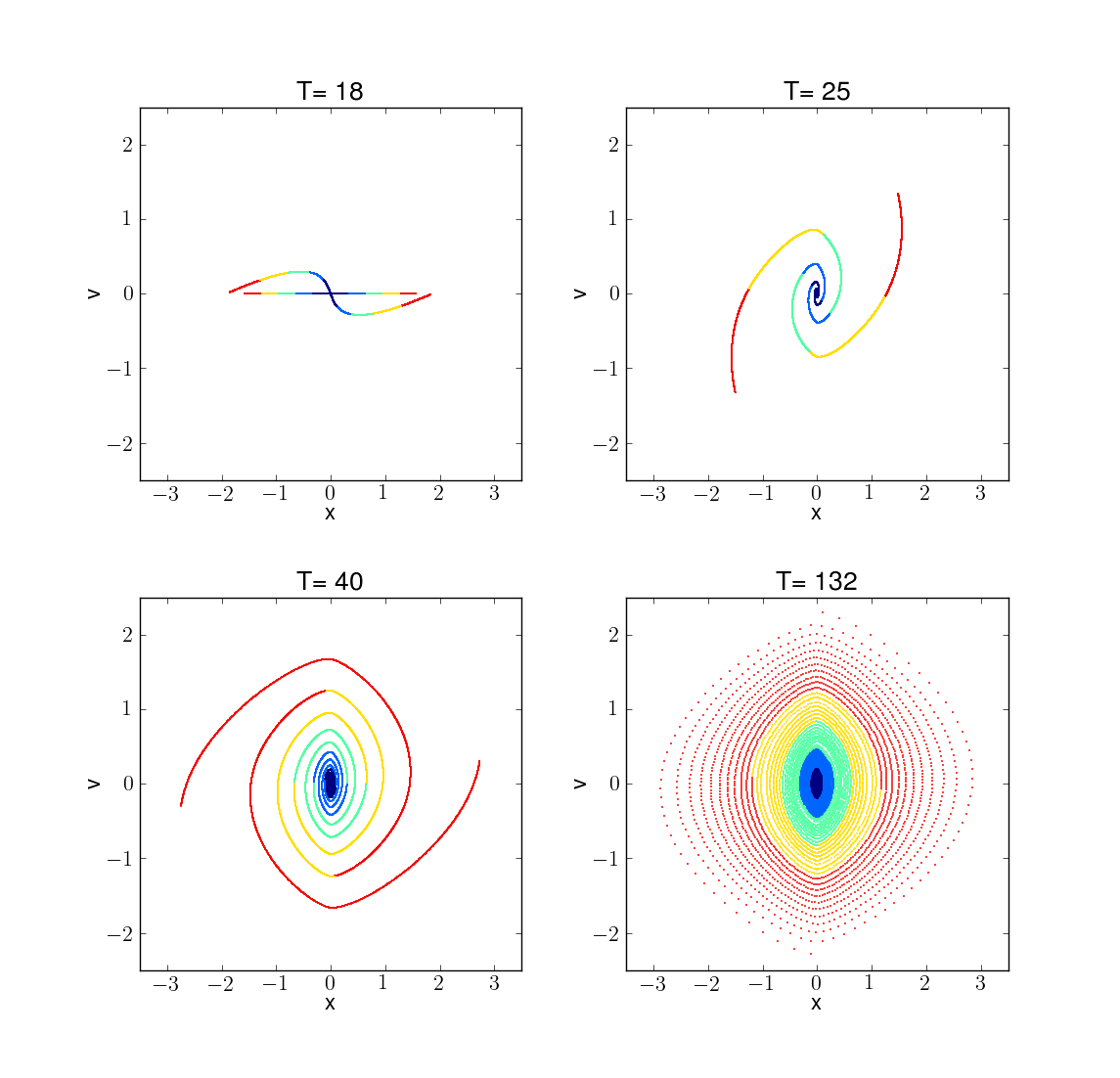
Early in the evolution, rapid changes in the gravitational potential cause energy transfer among the particles, leading to violent relaxation (Lynden-Bell, 1967). Note that the orbital specific energies of particles, , do not sum to the conserved total energy, , so the energy changes of particles need not sum to zero. During this period, the potential oscillates in time, with oscillations damping as the particles approach their final relaxed state. Violent relaxation ends when the particle locus is tightly wound and the gravitational potential is no longer changing significantly.
Although the gravitational potential approaches a stationary state, the spiral curve describing the locus of the particles continues to wind up. In the limit where the state is described by a continuous curve in the -plane, this spiral will continue winding indefinitely. In the simulated system, with a finite number of particles, the particle density along the spiral eventually decreases to the point where the curve is no longer identifiable; at this point, discreteness effects have erased any visual remnant of the phase coherence necessary to define such an approximate curve.
These simple observations are directly related to the meaning of convergence in the collisionless limit. In order to make contact with the stationary solutions of the collisionless Boltzmann equation (1), we must understand the nature of this convergence as . A state supported on a smooth curve in phase space formally has an infinite number of particles, but it never becomes stationary in a pointwise sense. Rather, in the collisionless limit, these states converge only weakly, as measures, to stationary solutions of the CBE (Braun & Hepp, 1977). Therefore, the winding spiral locus can be identified with a stationary solution only through a process of coarse-graining. Coarse graining need not be restricted to averaging over phase space coordinates, but could also be implemented by averaging over orbital phase. For example, the dependence in equation (13) relies on such a coarse graining.
4.2 Cold initial conditions with homogeneous density
4.2.1 The fiducial simulation
To obtain the density profile for the final state of cold collapse, we ran a suite of simulations, with particle numbers clustering around . The choice of in these simulations is discussed below. For our fiducial simulation, we chose and set the total mass to one, , implying a system of units where typical lengths and dynamical times are of order unity. The particles are initially equally spaced over the interval , and the initial velocities are set by
| (16) |
with the scaling factor . This state represents an initially overdense region near turnaround. The evolution of this state leads to a single collapsed object with a stationary profile. The simulations were run to time , although several results are reported at time . At time (), the outermost particles have executed roughly () orbits, with inner particles executing orders of magnitude more. The simulation at these times has evaluated approximately () particle crossings.
Fig. 2 shows the density profile of the equilibrated system. The number density is computed using bins of variable width, set down so that there are approximately 20 particles per bin, and the abscissae for these points are placed at the geometric mean of the bin edges. The curve is the average of six different simulations. As is clear from Fig. 2, the final state is self-similar over four orders of magnitude in distance from the center. The fine-scale structure in the average profile has two easily identifiable sources. First, the pointwise density profile for each simulation is dominated by caustics, the heights of which are regulated by the discreteness of the particle representation. Second, approximating the continuous density distribution along a curve in phase space by discrete particles leads to fluctuations in density because of counting statistics. The caustic structure is easily identifiable at early times, but at the time represented in the figure, the discreteness of particle sampling makes it impossible to identify individual caustics; in all likelihood there are multiple caustics per bin.
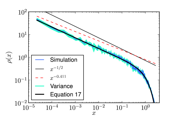
The density estimator for a single simulation approximates the continuum density profile but suffers from the fact that the bin spacing and the particle phases interact to produce slight (discretized) variations in the measured density in the bin. Roundoff error may also be responsible for occasionally pushing particles over the bin boundaries, a form of discretized phase error. To explore the impact of discretization and roundoff error, we have repeated the simulation with slightly different values of ; the six runs used to produce Fig. 2 have and . The bin positions are the same for all six simulations, allowing us to quantify the sensitivity of the density estimator to the types of phase errors probed by these different choices. The mean density obtained from these six simulations is shown in Fig. 2 as a jagged blue line. The uncertainty in the mean, estimated from the variance of the six runs, is shown as a shaded region. These “errors” are generally somewhat smaller than Poisson in the power-law region.
The fluctuations in the estimated density should not be interpreted as Gaussian random fluctuations. An Anderson-Darling test run on the 6 values of the density in each bin suggests that only a small fraction of the bins, less than 15%, are consistent with having been drawn from a Gaussian distribution. A histogram of the skewness of the 6 density measurements in each bin shows no net skewness; however, most of the bins show significant negative kurtosis (rounded peak with very short tails). Since fluctuations are principally generated by a small number of particles shifting across a single bin boundary due to phase differences, we would expect particle excursions to be at most one bin division and the tails of the distribution to be extremely small. We have checked that the distributions of skewness and kurtosis do not evolve as a function of distance; the inner decades display the same skewness and kurtosis properties as the outer decades. Therefore, we feel confident that we can use the measured variances as weights when fitting a power law of the form , without systematically over or under weighting any region of the data. However, it would be unwise to propagate errors from to errors on the fit parameters and , because such errors would be very difficult to interpret. For this reason, we use the bootstrap technique to generate a large number of mock datasets, with replacement. We use a least-squares procedure to fit the parameters for each of the mock datasets, and report the mean and variance of these fits to the synthetic data.
Using this method we have fit a power law to the portion of the data in the range . We find with a reduced , computed using the standard deviations within each bin. The small value of the reduced compared to the expected value arises from the negative kurtosis discussed earlier. The solid black line in Fig. 2 is obtained by multiplying this fit with a smooth truncation function (reminiscent of Einasto & Einasto 1972 models)
| (17) |
but the truncation of the power law in the outskirts is not the focus of our study. The fiducial simulation shows that the density follows a power law over at least four orders of magnitude in distance from the center, the extent of which is only limited by our finite resolution. This confirms the results of Binney (2004) with many more particles (301 vs. 40000 in our highest N simulation). However, the slope differs slightly but significantly from the value suggested by Binney, shown in Fig. 2 for comparison. There is a small systematic trend in the fit as a function of the range of data being fit; decreasing either the inner or the outer boundary causes to be slightly smaller (shallower), though in every case significantly different from .
4.2.2 Resolution study

| binned | single run | from | |||||
| 2000 | 0.3499 0.0302 | 0.4345 0.0255 | 0.6307 | 0.4778 0.0187 | 0.4699 0.0009 | 0.4828 0.0003 | 0.4155 0.0008 |
| 4000 | 0.3048 0.0065 | 0.4602 0.0043 | 0.2583 | 0.4710 0.0152 | 0.4602 0.0007 | 0.4499 8e-05 | 0.4129 0.0004 |
| 10000 | 0.3088 0.0043 | 0.4579 0.0031 | 0.3665 | 0.4703 0.0099 | 0.4567 0.0002 | 0.4378 1e-05 | 0.4115 0.0002 |
| 20000 | 0.2865 0.0015 | 0.4720 0.0014 | 0.3393 | 0.4722 0.0089 | 0.4497 0.0001 | 0.4478 8e-06 | 0.4110 8e-05 |
| 40000 | 0.2905 0.0007 | 0.4700 0.0006 | 0.3102 | 0.4691 0.0068 | 0.4491 7e-05 | 0.4606 4e-06 | 0.4107 4e-05 |
In Table 1, we show how these results depend on particle number over the range to . Columns 2 and 3 show the best fit values of the normalization and exponent of the density profile at time , Column 4 shows the reduced ; this should be roughly unity if the data are consistent with the fitted density profile and the errors are Gaussian. However, we expect to be less than 1 because the errors in the density bins show significant negative kurtosis. The apparent trend in and with is illusory; it is only the case for this particular snapshot. Although the smallness of the bootstrap errors indicate that the fit is very stable at a given snapshot in time, the value of the best fit varies from one snapshot to the next.
Fig. 3 plots the best fit value of for several snapshots with errors from the bootstrapped data, and demonstrates the extent of the time variability of the fit. Simulations with more particles display smaller absolute rms variability with time, but have a much larger disparity between the rms variability in time and the bootstrapped errors in a particular time step. This is because we have used a density estimator with approximately particles per bin for all resolutions in this study. Therefore the simulations with more particles have more data points available for the bootstrap. For all resolutions, however, the bin locations shift from one time step to the next, keeping the number of particles per bin roughly equal to . This procedure generates variability in the density estimator from one snapshot to the next. The time average and variance of over the interval are shown in column 5 of Table 1.
As discussed in section 2, a self-similar solution exhibits its power-law behavior in several different functional relations. In principle, the exponent can be extracted from measurements of any one of these relations. For example, the cumulative mass inside a position is . Since the mass is a cumulative variable, mass data points are correlated; however we have opted to give all points equal weight in the bootstrap procedure. We have computed the cumulative mass in two ways, first by numerically integrating the mean density (abscissae at the bin locations), and second by avoiding the binning entirely and tallying the total mass at the particle locations for one of the runs (abscissae at the particle locations). The results of fitting the cumulative mass can be found in columns 6 and 7 of Table 1. The exponents are not consistent with the fits to the density, nor with one another. This discrepancy is not understood, though it is easy to identify systematics which may affect the fit. Being an integrated quantity, the cumulative mass is sensitive to all regions of the data interior to ; in particular, it is not possible to excise the innermost part of the object as we have done with the density. Including more of the central region in the density fits will cause the power-law exponent to be systematically shallower than when it is excised, consistent with the mass result. The binning also likely affects the fit differently for the mass and the density.
The most interesting of the indirect scaling relations is that expressed in equation (13). The action of a particle orbit in the stationary mean-field potential can be computed directly by integration over the orbit. The values for exponents obtained by fitting this relation are shown in column 8 of Table 1 and show a remarkable stability as a function of , compared to the other methods. In Fig. 2, the density profile corresponding to this value of the exponent is indicated by the dashed line. The discrepancy between the direct fit to the density and the indirect fit to the relation is very clear in that figure. The details of the measurement and fit of the relation are discussed further in section 4.5.
4.2.3 Sensitivity to initial conditions
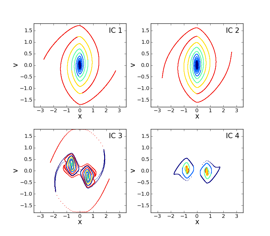
To close this section on simulations of cold collapse, we discuss the sensitivity of the exponent to changes in the initial conditions (ICs). Fig. 4 shows several of the initial conditions that we have tested. These are all cold and homogeneous in density, but with a variety of initial velocity perturbations. IC 0 is the fiducial case, with particle velocities given by equation (16) with . IC 1 tests the sensitivity to the velocity amplitude; IC 2 investigates the impact of a slow group of outer particles whose infall velocity lags that of intermediate particles; IC 3 has two additional inflection points away from the origin; IC 4 examines initially expanding rather than initially contracting particles.
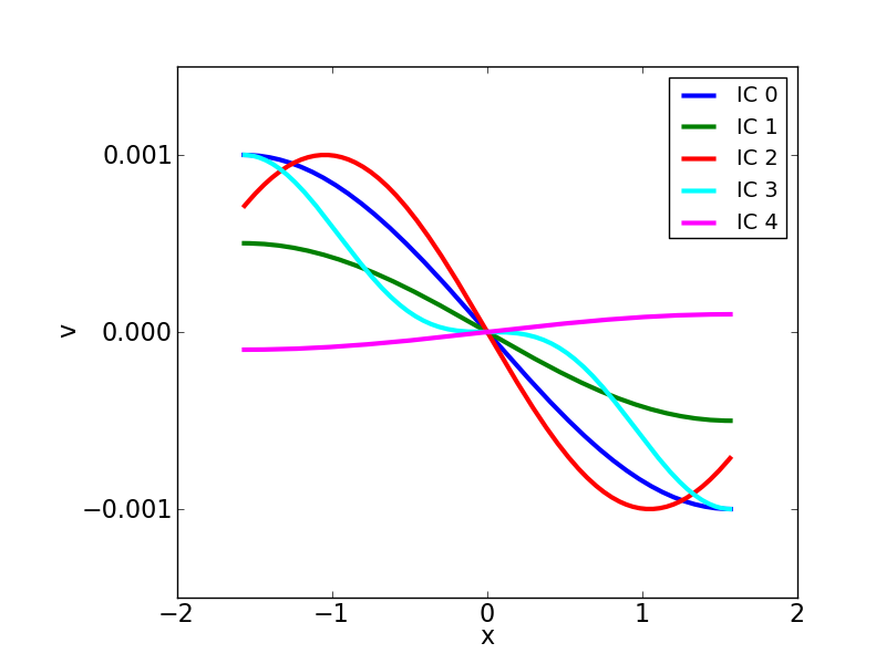
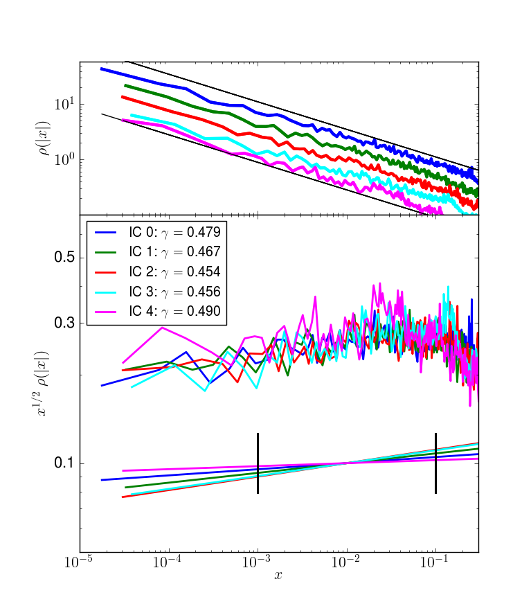
Fig. 5 shows the final configuration () of each IC. The top panel shows the average density of six simulations with the same number of particles as for the fiducial simulation, for each initial condition. The normalizations of all ICs except IC 0 have been artificially shifted for visual clarity. Solid black curves with power-law behavior are also shown for reference. The bottom panel shows the same average densities, but with an trend scaled out. The normalizations are not shifted in this panel. We see that the resulting density profiles for these different initial conditions are consistent with an attractor behavior with . Power laws with the best fit (in the legend) are plotted in the lower part of the bottom panel, to help quantify the extent to which the density approaches an attractor. The vertical black hashes show the range of data that was used in the fit. There is some covariance between the slope and the amplitude.
Even though the final states of these simulations are similar, there are large qualitative differences in the formation history. Fig. 6 shows an intermediate snapshot of the phase-space configuration for these four simulations; ICs 1 and 2 undergo a monolithic collapse, while ICs 3 and 4 each form two distinct halos that later merge to form the final product. These can be compared with the bottom left panel of Fig. 1, which shows IC 0 at the same time. The colors in Fig. 6 encode the initial positions of the particles; blue particles were initially located close to and red were at the largest distances. Note that the inner particles remain in the interior of the final halo only for cases that undergo monolithic collapse.
4.3 Warm initial conditions
The self-similar final states discussed above arise from cold initial conditions. At the end of Section 2, we described “coldness” as localization of the particle density to a single smooth curve in the -plane. In this section we describe simulations whose final states are quite different from the self-similar states described above. We assume in this discussion that a state initialized with velocity perturbations from a stochastic process (noise) satisfies any conceivable definition of “warm”. Our interest is in the approach to warmness as structure is added to the function describing the cold initial particle locus. We shall find that even a small amount of additional structure in the initial state, that appears consistent with the notion of “coldness,” destroys the self-similarity of the final state.
In a particle representation, the degree of smoothness of the particle locus must be compared to the particle separation. In the cold scenarios above, initial velocity perturbations were chosen to have wavelengths much larger than the initial particle separation. As the wavelength of the initial velocity perturbation decreases, it approaches the Nyquist limit for particle sampling, becoming more like a velocity noise in character. In this limit, we expect the subsequent evolution to resemble that of warm initial conditions, where the velocity perturbations are generated by independent stochastic processes for each particle. As a consequence, we expect that the resulting equilibrium halo will develop a core; collapse from a state of nonzero velocity dispersion should develop a core because the maximum phase-space density cannot increase (Tremaine & Gunn, 1979).
Fig. 7 shows the density profiles that result from adding an extra component to the velocity perturbation of equation (16).
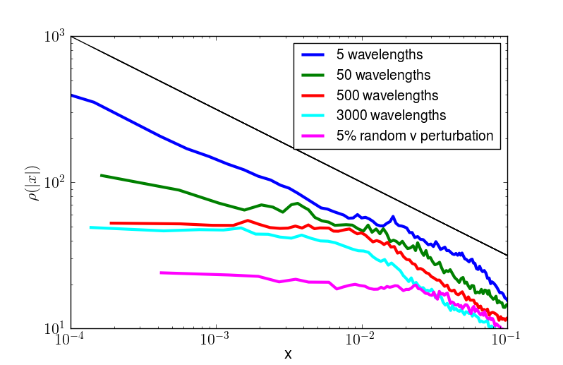
The additional component has a lower amplitude than the original perturbation (), but a higher wavenumber modulation. We have tested components containing 5, 50, 500 and 3000 wavelengths over the domain of the data; for comparison, the Nyquist rate (determined by the initial inter-particle spacing) would correspond to wavelengths over the domain of the initial particle distribution (). The bottom curve (magenta) shows a warm simulation in which an RMS 5% random fluctuation has been added to the initial velocities. These curves are averaged over six simulations and 20 time units (in the range 680-700) for reasons explained below. As expected, the density profile becomes shallower near the center as the spatial frequency of the initial velocity perturbation increases. These features indicate that it is difficult to achieve coldness in particle realizations of the continuum. It is remarkable that a well-defined constant-density core appears even in a simulation for which the spatial frequency is only 10% of the Nyquist frequency.
Less obviously, a high frequency perturbation in the initial velocities leads to the formation of substructures. This is illustrated in Fig. 8, which shows three successive times from the simulation plotted in blue of Fig. 7, in which the initial velocity perturbation contains five wavelengths in the domain of the initial particle distribution.

Many individual sub-halos form in locations where the flow is initially converging, before merging to form the final product. The sub-halos are very long lived; some of them never dissolve over the simulation times we have tested. Thus we can only measure a density profile in a time averaged sense—this is why 20 time units have been averaged to produce the curves in Fig. 7.
4.4 Cold initial conditions with inhomogeneous density
All simulations discussed thus far were initialized with constant density. In this section we report on simulations initialized with an inhomogeneous density. In particular, we choose an initial power-law density profile . We will demonstrate an apparent bifurcation in the form of the final state as a function of the initial exponent . The simulations described here all had and particles, with particle spacing chosen so that the resulting density is a power law with exponent .
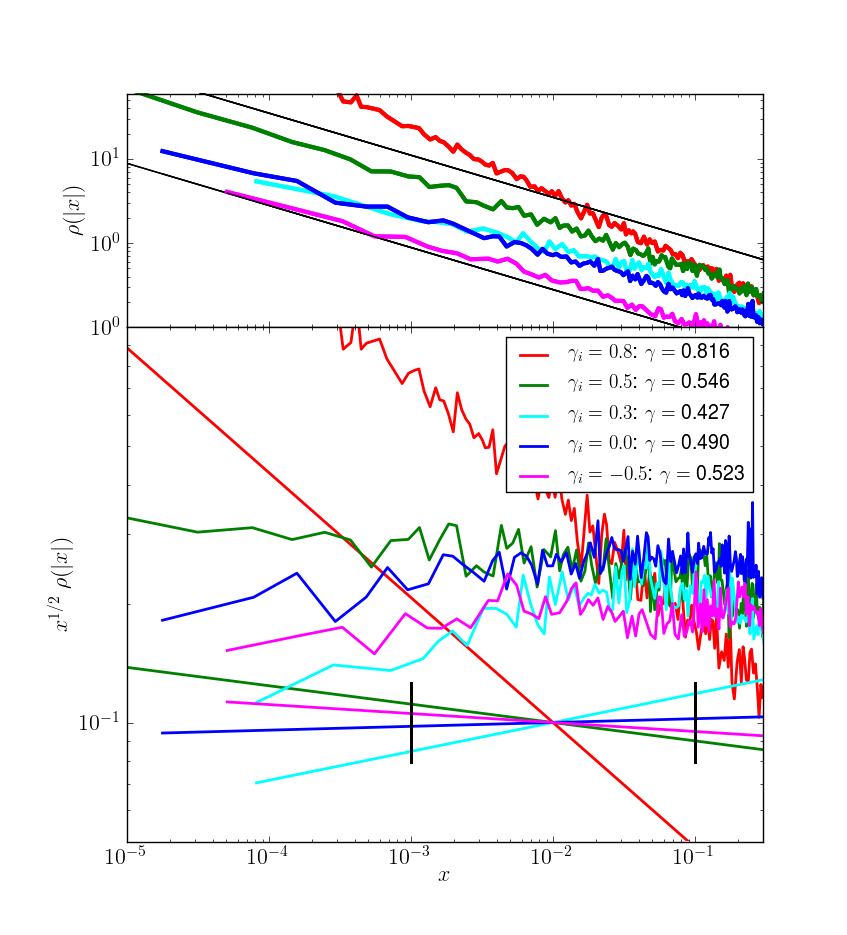
Fig. 9 summarizes the results of a set of simulations with initial exponents . The curve labeled shows our fiducial simulation for comparison. All initial particle velocities were set to in these simulations (except the fiducial case). We find that initial conditions with slope collapse to form final states with roughly the same density profile as homogeneous initial states, shown in dark blue in Fig. 9. However, initial conditions with , such as the red curve in Fig. 9, all preserve their density profiles. The bottom panel of Fig. 9 shows that the attractor is not as tight as in the homogeneous case; the curves do not overlay one another as tightly as in Fig. 5, and there is more scatter in the measured power law index. Also the central portions of the profile appear to be flatter than the behavior at larger . For this reason the fit values (displayed in the legend) are somewhat more sensitive than fits in Fig. 5 to the range of data used in the fit (indicated in the bottom panel of Fig. 9 with short vertical black lines).
Fig. 10 shows the exponent of the final density profile, , versus that of the initial condition for a larger set of values of . Each data point is computed using 6 simulations. For these simulations, we have perturbed the particle velocities according to equation (16), because this significantly decreases the run time. For the cases with , we have verified that the velocity perturbation does not significantly impact the measured slopes. Solid lines for and are also plotted for reference.
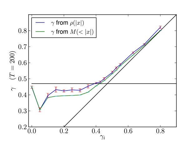
Although the bootstrap method significantly reduces the sensitivity to the range of data used for the fits in Fig. 10, it does not eliminate it entirely. If either the inner or outer boundary of the domain is reduced by an order of magnitude or more, the best fit becomes systematically shallower. The fitted exponents in Fig. 10 are power-law fits to the portion of the density in the range . The figure suggests that a system initialized in a more collapsed state than the attractor solution remains close to its initial power law. However, a system initialized with a shallower density profile than the attractor significantly steepens to evolve toward the attractor. The dip of very shallow slopes for has its origin in two features of these final states. First, at the simulations with display noticeable gaps in phase space structure in the range . These gaps, and similar gaps in the homogeneous simulations, are discussed below. These gaps affect the fit for the exponent. Second, simulations with achieve much lower peak phase-space densities than the homogeneous case or cases with . We postulate that either the gaps or other discreteness effects interfere with the efficient transfer of energy from the inner particles to the outer ones. Since the inner threshold is fixed, we are not discarding the very innermost portion of the data in these simulations, and the fits result in systematically shallower values of , as discussed above.
4.5 Time evolution of rank, action, energy and density
Fig. 11 shows the evolution of the particle energies and actions as a function of time. The different colors mark quintiles in the initial particle position, as described in Section 3. The evolution of the energies for the fiducial simulation, in the top left corner, shows rapid oscillations for . The phase space plots of the system configuration can be seen in Fig. 13, at the times indicated by the vertical magenta lines. Before time , the system is undergoing rod-like rotation in phase space, with only one stream per location . The oscillations in the energy are dominated by changes in the potential, as the system oscillates between maximum rarefaction and maximum compression. At approximately , the system transitions from one to three streams at small . After this time the central part of the particle locus winds up quickly, with more than streams in the inner region by time , but the oscillation pattern in energy continues in phase with the outer particles, suggesting that the potential in the center is dominated by the configuration of the particles in the outskirts at these times. The range of particle energies spreads with time, indicating that energy is being transferred from inner to outer particles. The colors are not mixed, demonstrating that the particles approximately maintain their rank ordering in energy; violent relaxation redistributes energy among the particles but does not scramble the energy ordering. For the energies of the particles are nearly constant. For example, an extended run shows that the energies of the (most, least) energetic particles change by (0.5%,1.0%) between 150 and 700 time units. This simulation was run for several values of , as indicated in Table 1. The energy oscillations from violent relaxation occur in phase for all of these runs, and the final energies of the (innermost, outermost) particles of the two highest resolution runs match to within (0.7%, 0.6%) in all the simulations.
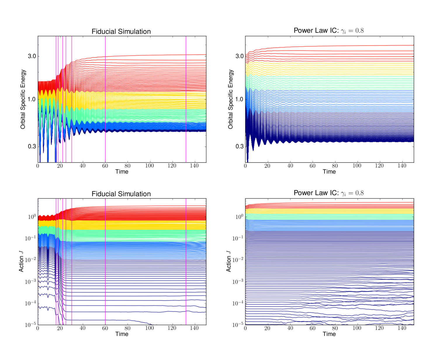
The time evolution of the particle actions in the fiducial simulation is shown in the bottom left hand panel of Fig. 11. The actions are computed assuming the potential is fixed at its instantaneous functional form, even though for times less than the potential is evolving significantly. The fluctuations in low at late times are almost certainly caused by discreteness noise. The actions display a number of interesting features. First, they stabilize extremely abruptly, well before the energy oscillations damp out and the energies of the particles cease to evolve. Second, the transition to constant action for the inner particles happens just after the transition from rod-like rotation to multiple stream flow. This can be seen in the fiducial simulation by comparing to the top row of Fig. 13, which shows that the transition from rod-like rotation to multi-stream flow happens at approximately time .
Comparing the energy and action plots we learn that the relaxation of the system appears to be a two stage process. The first stage, in which both the energies and the actions evolve rapidly, happens primarily before the transition from one to three streams. The second stage, in which the actions rapidly settle and the energies evolve adiabatically, happens as the system winds up, primarily between the one-to-three stream transition, and the ultimate stabilization of the outer gravitational potential. During this second stage, the amount of energy transferred between particles, and the distances over which it can be transferred both tend to zero as the number of streams increases and the inter-caustic distance decreases.
The panels on the right of Fig. 11 show the evolution of the particle energies and actions for one of the simulations initialized with a steep power law density profile. These plots contrast starkly with the evolution of the fiducial simulation. We see that the actions (bottom right panel) are immediately stable, and evolve very little from their initial values. This is the case because the one-three stream transition occurs well before time , and the system does not undergo several rod-like rotations before the transition to multiple streams. Therefore, steep systems like this one relax mainly through the second adiabatic stage of energy redistribution. The redistribution of particle energies (top right panel) is much less than in the fiducial case. Since the particles are essentially in fixed stable orbits from time onward, the change in the scaling of the density profile is small, as can be seen in Fig. 10.
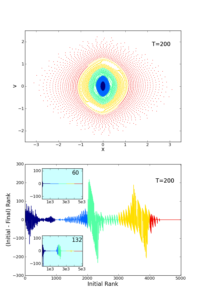
A curious feature in the top left panel of Fig. 11 is the development of narrow gaps in the energy distribution, seen after about 60 time units, in the yellow and green curves. The gaps correspond to specific phase space pockets, empty of particles, which open at times significantly after the end of violent relaxation. An example can be seen in the top panel of Fig. 12. The emergence of these gaps scrambles the energy rank-ordering of the particles that had been preserved in the earlier stages of the evolution (bottom panel).
These gaps are a robust result of our simulations. We observe them in simulations with all values of , with and without imposing explicit left/right symmetry, and gaps appear in both the heap and the search-tree versions of the code run on identical initial conditions. They also occur in the simulations initialized with a power law density profile, though they manifest at different times and are much less pronounced when the initial density profile is steep.
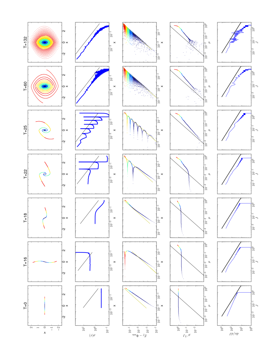
Fig. 13 shows the state of the fiducial system at 8 specific times, which are indicated in the left panels of Fig. 11 with vertical lines. The phase-space distribution (first row) is shown with color indicating quintiles in initial position. The evolution of the density profile (second row) shows the steady growth in the number of caustics. At early times the density is roughly constant in the intervals between caustics. As the evolution proceeds, the caustics become more closely spaced and the usual density distribution associated with a fold singularity at dominates the behavior between caustics. We also notice that the caustics are roughly equally spaced in logarithmic distance.
Also shown in Fig. 13 are plots of energy versus position for the particles (third row). The colors in this row again indicate quintiles in initial particle position. As seen in these plots, violent relaxation mixes the final positions relative to the initial ones (the colors are mixed when projected onto the horizontal axis) but does not mix the final energies relative to the initial ones (the colors are not mixed when projected onto the vertical axis). The envelope of the energy-position plot gives the maximum orbital excursion as a function of energy; the locus of this envelope is the potential as a function of distance, and therefore displays the power-law behavior . For comparison, this form of the potential is shown with a green line. Indeed, if the turnaround is known for all the particles, this behavior can be used as another method to infer . We examined this for the fiducial simulations and found that the power law is slightly shallower than when fitting the cumulative mass, though not as shallow as when fitting . Since the potential is a double integral of the density, it displays correlations and dependency on the global structure of the state, similar to the effects discussed for the cumulative mass scaling in section 4.2.
The evolution of the relation is displayed in Fig. 13 (fourth row) and shows a very clean power law developing even before the end of violent relaxation (). Here we have scaled by so that the initial relation is flat. The solid black line shows the scaling from equation (13) for the value , demonstrating that the asymptotic scaling of this relation predicts a different value of than the other scaling relations. The power-law behavior develops much earlier than the time at which power-law behavior in the density becomes apparent. The panel at shows that this power-law behavior is first seen in the outer parts of the system and last established in the inner parts, which is perhaps somewhat counterintuitive. This dynamical behavior is related to the fact that the phase-line remains close to a straight line longest at . The clean power law in deteriorates at later times, apparently due to the loss of coherence in the center of the system, consistent with the loss of correlation between and particle energy.
As already indicated in Table 1, the value of the exponent extracted from the measured relation is systematically lower than that extracted from fits to the density. However, these exponents cannot be compared at the same times, because the relation deteriorates before the density is sufficiently settled. All fits to the relation referred to in this paper have been done at times around to allow sufficient dynamic range for an accurate fit, . However, the observed slope of does not appear to evolve at all past this time, and it is easy to conjecture that a simulation with sufficient resolution in the center to delay the deterioration would show no subsequent change or drift in the exponent determined from . We conjecture that the reason the exponent obtained from does not agree with fits to the density is because the monotonicity of the relation is destroyed by discreteness effects (see bottom panel of Fig. 11) well before the system is sufficiently wound to render the expression in equation (13) valid.
The bottom row in Fig. 13 shows the evolving distributions of orbital actions (per unit ); we expect a coarse-grained power-law behavior as expressed in equation (12). This is shown in the plot with a solid black line for . The observed distribution shows clear systematic deviations from the expected power law at intermediate times and becomes sufficiently disordered at later times that it is impossible to extract a meaningful value of . Although we might expect certain subtleties in the convergence of the distribution in , it is somewhat surprising that this distribution can display such complex structure, while the observed relation is quite stable and clean.
We do not show similar snapshots for the simulations initialized with a power-law density profile; however, we now describe the results qualitatively. The violent relaxation and settling to an equilibrium gravitational potential proceed much faster in simulations with a steep initial profile compared to those with a shallow initial profile. The development of gaps of the type shown in Fig. 12 is strongly suppressed in the steep cases, compared to the shallow cases. Finally, there is a difference in the evolution of the distribution of actions: the shallow cases eventually reach an distribution that follows equation (12) with respect to the final slopes of the density profiles. However, the steep cases do not. The distribution for the steep cases begins very close to the that would be expected for a scaling, and since the actions retain their initial values (shown in Fig. 11), this distribution does not evolve at all.
5 Conclusions
We have performed a suite of simulations of one dimensional gravitational collapse, equivalent to infinite parallel mass sheets collapsing along one axis in three dimensions. We find that a self-similar attractor solution exists for “cold” initial conditions with near-homogeneous density; the density in the final state attractor follows a power law, , over at least three decades of distance, with . The measured value of the exponent is shallower than the value conjectured by Binney (2004). This self-similar state arises after a period of violent relaxation that redistributes energy while preserving the energy ranking of the particles. The measurements of the exponent for the power-law density profile are done at times significantly after the end of violent relaxation ( versus ), to ensure that the coarse-grained density has achieved a stationary form. Measurements of the exponent obtained from the relation can (and must) be done at significantly earlier times. These show that an attractor solution is in place at very early times. However, the exponent obtained from is systematically lower than that obtained from the density at later times. The two determinations cannot be compared because at later times discreteness effects destroy the phase coherence of the simulations, and with it the monotonicity of . If the initial conditions are warmed by applying smooth velocity perturbations with spatial frequencies approaching the Nyquist limit, a cross-over is reached where self-similarity of the final state is destroyed and is replaced by a cored solution. Cold initial conditions with a steep initial power-law density of exponent do not reach the attractor either; they instead collapse to form a final equilibrium state with .
Our simulations provide some insight into the process of violent relaxation and provide hints that may be useful for the development of an analytical understanding of the properties of the attractor solution. For example, we find that many of the scaling laws are in place very early, even during the violent relaxation process. The evolution of some of the scaling relations suggests that the violent relaxation process finishes first in the outer parts of the structure, while the inner particles take longer to redistribute their energies. Such insights may then also be extended to the 3D case, eventually shedding light on the origin of cold dark matter halo density profiles.
Acknowledgments
The authors thank Daniel Holz, Doug Rudd, Mike Warren, and Nadia Zakamska for inspiring and helpful conversations. A.E.S. was supported in part by the Corning Glassworks fellowship and the National Science Foundation.
References
- Binney (2004) Binney J., 2004, Mon. Not. R. Astron. Soc., 350, 939
- Binney & Tremaine (2008) Binney J., Tremaine S., 2008, Galactic Dynamics: Second Edition, Princeton University Press
- Braun & Hepp (1977) Braun W., Hepp K., 1977, Communications in Mathematical Physics, 56, 101
- Cuperman et al. (1969) Cuperman S., Goldstein S., Lecar M., 1969, Mon. Not. R. Astron. Soc., 146, 161
- Dalal et al. (2010) Dalal N., Lithwick Y., Kuhlen M., 2010, ArXiv e-prints, arXiv:1010.2539
- Dehnen & McLaughlin (2005) Dehnen W., McLaughlin D. E., 2005, Mon. Not. R. Astron. Soc., 363, 1057
- Diemand et al. (2008) Diemand J., Kuhlen M., Madau P., et al., 2008, Nature, 454, 735
- Dobler et al. (2010) Dobler G., Finkbeiner D. P., Cholis I., Slatyer T., Weiner N., 2010, Astrophys. J., 717, 825
- Doroshkevich et al. (1980) Doroshkevich A. G., Kotok E. V., Poliudov A. N., Shandarin S. F., Sigov I. S., Novikov I. D., 1980, Mon. Not. R. Astron. Soc., 192, 321
- Einasto & Einasto (1972) Einasto J., Einasto L., 1972, Tartu Astrofuusika Observatoorium Teated, 36, 3
- Gabrielli et al. (2009) Gabrielli A., Joyce M., Sicard F., 2009, Phys. Rev. E, 80, 4, 041108
- Gurevich & Zybin (1995) Gurevich A. V., Zybin K. P., 1995, Physics-Uspekhi, 38, 7, 687
- Hooper et al. (2007) Hooper D., Finkbeiner D. P., Dobler G., 2007, Phys. Rev. D, 76, 8, 083012
- Kandrup (1998) Kandrup H. E., 1998, Astrophys. J., 500, 120
- Lecar & Cohen (1971) Lecar M., Cohen L., 1971, Ap&SS, 13, 397
- Lynden-Bell (1967) Lynden-Bell D., 1967, Mon. Not. R. Astron. Soc., 136, 101
- Maciejewski et al. (2011) Maciejewski M., Vogelsberger M., White S. D. M., Springel V., 2011, Mon. Not. R. Astron. Soc., 415, 2475
- Merritt et al. (2006) Merritt D., Graham A. W., Moore B., Diemand J., Terzić B., 2006, Astron. J., 132, 2685
- Mineau et al. (1990) Mineau P., Feix M. R., Rouet J. L., 1990, Astron. Astrophys., 228, 344
- Navarro et al. (1996) Navarro J. F., Frenk C. S., White S. D. M., 1996, Astrophys. J., 462, 563
- Noullez et al. (2003) Noullez A., Fanelli D., Aurell E., 2003, Journal of Computational Physics, 186, 697
- Rybicki (1971) Rybicki G. B., 1971, Ap&SS, 14, 56
- The Fermi-LAT Collaboration: M. Ackermann et al. (2011) The Fermi-LAT Collaboration: M. Ackermann, Ajello M., Albert A., et al., 2011, ArXiv e-prints, arXiv:1108.3546
- Tremaine & Gunn (1979) Tremaine S., Gunn J. E., 1979, Physical Review Letters, 42, 407
- Vogelsberger & White (2011) Vogelsberger M., White S. D. M., 2011, Mon. Not. R. Astron. Soc., 413, 1419
- Yawn & Miller (1997) Yawn K. R., Miller B. N., 1997, Phys. Rev. E, 56, 3, 2429