An extended density matrix model applied to silicon-based terahertz quantum cascade lasers

Abstract

Silicon-based terahertz quantum cascade lasers (QCLs) offer potential advantages over existing III–V devices. Although coherent electron transport effects are known to be important in QCLs, they have never been considered in Si-based device designs. We describe a density matrix transport model that is designed to be more general than those in previous studies and to require less a priori knowlege of electronic bandstructure, allowing its use in semi-automated design procedures. The basis of the model includes all states involved in interperiod transport, and our steady-state solution extends beyond the rotating-wave approximation by including DC and counter-propagating terms. We simulate the potential performance of bound-to-continuum Ge/SiGe QCLs and find that devices with 4–5-nm-thick barriers give the highest simulated optical gain. We also examine the effects of interdiffusion between Ge and SiGe layers; we show that if it is taken into account in the design, interdiffusion lengths of up to 1.5 nm do not significantly affect the simulated device performance.

I Introduction

Terahertz quantum cascade lasers (THz QCLs) are compact, coherent radiation sources in which electrons are transported through a periodic semiconductor heterostructure, with a radiative transition in each period.NatureKohler2002 Silicon-based THz QCLs may offer significant advantages over the existing III–V devices including the absence of Reststrahlen absorption, which may allow emission at frequencies above the current limit of 4.9 THz in GaAs/AlGaAs QCLs.APLLee2006 III–V devices require cryogenic cooling (currently to $<200$ KOptExpFathololoumi2012 ) but the high thermal conductivity of Si and the absence of polar LO-phonon interactions could potentially overcome this limitation. Additionally, there is the prospect of leveraging the mature Si process technology, to create affordable integrated electrically-driven semiconductor THz lasers. Although mid-infraredScienceDehlinger2000 and THzAPLLynch2002 electroluminescence from $p$-type SiGe/Si quantum cascade structures has been achieved, lasing has not yet been demonstrated. In recent years, attention has switched to $n$-type devices owing to the simpler electron dispersion. We recently showed theoreticallyPRBValavanis2011 that the low effective mass and large usable conduction band offsets of the $L$-valleys in Ge/GeSi heterostructuresAPLLever2009 ; APLDriscoll2006 could allow significantly higher gain, operating temperature and emission frequency range than equivalent Si/SiGe devices.IJHSESKelsall2003 ; PRBValavanis2008_2 ; APLLever2008

Several theoretical studies of Si-based QCLs exist,PRBValavanis2011 ; APLLever2009 ; APLDriscoll2006 ; JAPDriscoll2007 ; PRBValavanis2008_2 ; APLLever2008 ; APLSun2007 but none have accounted for coherent transport effects (i.e., quantum tunneling and interactions with optical fields). Although semiclassical scattering-transport models can give good agreement with experimental results,NatureKohler2002 ; JAPJovanovic2006 they neglect tunneling across barriers, and can predict unrealistically large spikes in current density and gain when electrons scatter between spatially-extended subbands.JAPCallebaut2005 By contrast, simplified density matrix (DM) modelsJAPCallebaut2005 ; APLKhurgin2009 ; PRBKumar2009 ; Dupont2010 ; Terazzi2010 ; Talukder2011a ; Talukder2011b account for tunneling, in addition to scattering, and include the effect of the optical field on the electron dynamics. Additionally, DM models are much faster and less computationally demanding than full quantum mechanical simulations based on Green’s functions.Wacker2002 ; Kubis2008 ; Kubis2009a ; Yasuda2009 ; Savic2007 ; Weber2009 To our best knowledge, all existing DM models of QCLs consider coherence between a reduced set of basis states including a single “injector” state (adjacent to a thick tunneling barrier) and a number of states in the next period of the QCL. This requires the manual selection of the injector state prior to simulating the device, and omits tunneling through the injection barrier from other states. This approach is not well-suited to semi-automated design procedures,Ko2010 ; PRBValavanis2011 and can be problematic in bound–to–continuum (BTC) designs, in which multiple states may contribute to the tunneling current. Furthermore, these simplified models neglect coherences between the injector state and other states in the same period. In this work, we present a generalized DM model that reduces the requirement for a priori knowledge of the electronic bandstructure by including all states involved in interperiod transport, and by including contributions from both the optical field and the external DC bias in all density terms in our steady-state solution.

Although the thickness of the injection barrier is of great importance in III–V QCls,Elec_Lett_Luo_2007 it has never been investigated in Ge/GeSi devices. We therefore use our DM model in conjunction with a semi-automated design algorithmKo2010 to investigate the influence of injection barrier thickness upon the simulated device performance. Ge/GeSi interfaces also exhibit significantly more elemental interdiffusion than the GaAs/AlGaAs epitaxy used in existing QCLs. We use our DM model to assess the effect of interdiffusion on the simulated population inversion and gain and we compensate for the gain-reduction through design optimization.

II Theoretical model

II.1 Bandstructure calculation

The optically-active region of a QCL consists of a periodic semiconductor heterostructure. In the DM model, the “injection barrier” that separates periods of the structure is assumed to be sufficiently thick that interperiod transport is limited to quantum tunneling only. QCL periods may be further subdivided into a number of modules that are separated by thick tunneling barriers.

We used a model-solid approximation to determine the conduction band profiles for the QCL structures in our simulationsPRBVanDeWalle1986 with the bandstructure parameters listed in Ref. PRBValavanis2011, . A self-consistent one-dimensional Poisson–Schrödinger solver was then used to locate the quasibound states within each module of the device, giving a total of $N$ subbands within each period. Localized wavefunctions $\psi_{i}(z)$ with energies $E_{i}$ were obtained, according to a ‘tight-binding’ scheme, by embedding each module of the structure between a pair of thick barriers, such that the amplitude of the evanescent waves decays to zero before reaching the edge of the simulation domain. Here, the subscript $i\in[1\ldots N]$ denotes the index of each state in the period, in ascending order of energy. Intervalley mixing has previously been shown to yield negligibly small energy splitting for intersubband transitions in Si-based heterostructures longer than a few nanometers,PRBValavanis2007 ; PRBVirgilio2009 and we therefore omit the effect from our model.

As the QCL is a periodic heterostructure in an electric field, the states localized in other periods of the device are obtained by simple translations of these solutions in energy and space. The $p^{\text{th}}$ downstream period of the cascade therefore has states with energy $E_{i}^{(p)}=E_{i}-eFLp$, where $F$ is the applied electric field, $e$ is the unit charge, and $L$ is the length of a period. The corresponding wavefunctions are given by $\psi_{i}^{(p)}(z)=\psi_{i}(z-Lp)$. The wavefunction for an electron in the system is expressed in this basis as

$$\Psi(z)=\sum\limits_{i=1}^{N}\sum\limits_{p=0}^{P}c_{i}^{(p)}\psi_{i}^{(p)}(z),$$ (1)

where $c_{i}^{(p)}$ is the weighting of each basis state and $P$ is the number of periods contained in the model.JAPCallebaut2005

II.2 Density matrix formulation

Density matrix calculations rely on the selection of suitable basis states for coherent transport through the QCL. Conventional approaches use $N$ basis states to model transport across a single injection barrier. A single “injector” subband is selected from the period upstream of the barrier. The remaining $N-1$ states are then selected from the period after the barrier, and the coherences between these states and the injector describe interperiod tunneling transport. Some approaches simplify the calculation further by selecting only a subset of the states from the period after the barrier. The manual selection of an “injector” subband requires a priori knowledge of the electronic bandstructure, and is therefore incompatible with semi-automated design optimization techniques. Even with a priori knowledge, the selection of an injector state may not be obvious, particularly when the QCL is biased well away from subband alignment; indeed, multiple channels for interperiod transport may exist. Also, this limited set of basis states does not include the injector subband in the second period. Although the effect on relaxation rates is included implicitly in the simulation, the calculation still does not account for any coherent interactions with this subband. Its role in intraperiod tunneling transport and its contribution to resonant optical transitions are therefore omitted.

Here we describe a different DM model that uses all the subbands localized in three adjacent periods of the QCL as its basis. This method allows coherences to be calculated between all pairs of states in the central period, and allows interperiod tunneling (both in and out of the central period) to be determined without the need to select an injector subband manually. The resulting $3N\times 3N$ density matrix may be expressed in block form as

$$\mathsf{\rho}=\begin{pmatrix}\mathsf{\rho}_{\text{CC}}&\mathsf{\rho}_{\text{CU}}&\mathsf{\rho}_{\text{CD}}\\ \mathsf{\rho}_{\text{UC}}&\mathsf{\rho}_{\text{UU}}&\mathsf{\rho}_{\text{UD}}\\ \mathsf{\rho}_{\text{DC}}&\mathsf{\rho}_{\text{DU}}&\mathsf{\rho}_{\text{DD}}\end{pmatrix},$$ (2)

where the subscripts $U$, $C$ and $D$ denote the upstream, center and downstream periods of the structure respectively. Each of these $N\times N$ blocks consists of density terms for pairs of states in the periods denoted by the block subscripts, for example,

$$\mathsf{\rho}_{\text{CC}}=\begin{pmatrix}\rho_{1,1}&\ldots&\rho_{1,N}\\ \vdots&\ddots&\vdots\\ \rho_{N,1}&\ldots&\rho_{N,N}\end{pmatrix}.$$ (3)

The density terms are unknown values to be solved, which represent the ensemble average of the weightings for the basis states $\rho_{i,j}=\overline{c^{*}_{i}c_{j}}$.

The Hamiltonian for the three-period system is written in block form as

$$\mathsf{H}=\begin{pmatrix}\mathsf{H}_{\text{CC}}&\mathsf{\Omega}_{\text{CU}}&\mathsf{\Omega}_{\text{CD}}\\ \mathsf{\Omega}_{\text{UC}}&\mathsf{H}_{\text{UU}}&\mathsf{\Omega}_{\text{UD}}\\ \mathsf{\Omega}_{\text{DC}}&\mathsf{\Omega}_{\text{DU}}&\mathsf{H}_{\text{DD}}\end{pmatrix}.$$ (4)

Here, the off-diagonal blocks contain the Rabi frequency terms for coupling between states in different periods of the QCL, which were calculated according to the scheme in Ref. Yariv1985, . The diagonal blocks such as $\mathsf{H}_{\text{CC}}$ denote the Hamiltonian matrix for a single period of the structure. The elements of these single-period Hamiltonians are either the basis state energies (for diagonal elements), the Rabi frequency terms (for pairs of states in different modules) or the optical-coupling terms $H_{i,j}=z_{i,j}A_{\text{inc}}$ for radiative transitions between states in response to incident light with the electric field $A_{\text{inc}}=A_{0}\exp(\mathrm{i}\omega_{0}t)$. Here, the dipole matrix element terms are given by $z_{i,j}=\left\langle\psi_{i}|z|\psi_{j}\right\rangle$.

The time evolution of the density matrix is expressed by the Liouville equation

$$\frac{\partial\mathsf{\rho}}{\partial t}=-\frac{\mathrm{i}}{\hbar}\left[\mathsf{H},\mathsf{\rho}\right]-\left(\frac{\partial\mathsf{\rho}}{\partial t}\right)_{\text{relax}},$$ (5)

where the last term is the matrix containing all relaxation and dephasing times.

Although the Liouville equation for our three-period model contains a total of $9N^{2}$ differential equations (compared with $N^{2}$ for a single-period model), the translational invariance of the system simplifies the calculation considerably. Firstly, the density terms may be translated between blocks of the matrix, such that $\mathsf{\rho}_{\text{UU}}=\mathsf{\rho}_{\text{CC}}=\mathsf{\rho}_{\text{DD}}$, $\mathsf{\rho}_{\text{CD}}=\mathsf{\rho}_{\text{UC}}$, and $\mathsf{\rho}_{\text{DC}}=\mathsf{\rho}_{\text{CU}}$. Similar translations may also be applied to the Rabi frequencies, dipole matrix elements, and relaxation times. The Liouville equation (5) can therefore be reduced to $3N^{2}$ independent differential equations, coming from the three blocks in the upper left corner of Eq. (2) and (4). Secondly, we apply the nearest-neighbor approximation, so that there is no coupling or scattering between states spaced by more than by one period. Therefore, the coupling constants between the first and third periods $\mathsf{\Omega}_{\text{DU}}$ are set to zero in Eq. (4), and the same applies to the coherence and relaxation terms. These simplifications reduce the computational complexity of our model to a level comparable with the single-period model.

The relaxation matrix can be written symbolically in the form

$$\tau^{-1}=\left[\begin{array}[]{ccc}\left(1/\tau_{\text{CC}},1/\tau_{\|\,\text{CC}}\right)&\left(1/\tau_{\|\,\text{CU}}\right)&-\\ \left(1/\tau_{\|\,\text{UC}}\right)&-&-\\ -&-&-\end{array}\right]$$ (6)

where the dashes indicate that the corresponding $N\times N$ block is irrelevant owing to translational invariance. The relaxation terms in Eq. (6) determine both the linewidths of optical transitions and tunneling lifetimes. They contain contributions from the state lifetimes $\tau_{i,j}$, as well as ‘pure dephasing’ times $\tau_{\|\,i,j}$ for intraperiod transitions.JAPCallebaut2005 The off-diagonal blocks in Eq. (6) (denoted $\tau_{\|\,\text{UC}}$, etc) describe the pure dephasing for interperiod interactions.

In this work, subband relaxation rates and tunneling dephasing rates were calculated by accounting for all relevant scattering processes:PRBValavanis2011 acoustic and optical phonon scattering, intervalley scattering, ionized impurity and interface roughness scattering. The pure dephasing contributions are not straightforward to calculate, and a number of different schemes for their estimation have been proposed.APLKhurgin2009 ; Talukder2011a ; Talukder2011b In the case of tunneling transitions, the prescription from Refs. Talukder2011a, ; Talukder2011b, was employed. In case of optical transitions, however, we have simply set the linewidths to 2 meV (as is typical for GaAs THz QCL structures).NatureKohler2002

II.3 Steady-state solution

The harmonic balance method is a convenient approach for determining a steady-state solution of the Liouville equation. Here, a simple steady-state functional form is assumed for each element of the density matrix depending on the states involved. Under the rotating-wave approximation (RWA), each element is assumed to contain only a single frequency harmonic. The diagonal elements of the density matrix $\rho_{i,i}$ give the state populations, and are assumed to be constant-valued. The off-diagonal terms $\rho_{i,j}$ describe coherences between states. In the RWA approach, the steady-state forms of these terms are selected depending on whether they are optically-active or not. It is assumed that pairs of states within the same period with an energy separation $E_{ij}\sim\hbar\omega_{0}\pm\Gamma$ will interact strongly with the driving optical field (including a transition linewidth $\Gamma$). The density matrix terms for optical transitions are assumed to be proportional to $\exp(\mathrm{i}\omega_{0}t)$ for $E_{i}<E_{j}$ or $\exp(-\mathrm{i}\omega_{0}t)$ for $E_{i}>E_{j}$. All other off-diagonal elements, (i.e. for pairs of states with small energy separations, or in different modules of the structure) are assumed to represent tunneling transport and are assumed to be constant valued. With the single dominant harmonic assumed for each $\rho_{i,j}$, the Liouville equation becomes a system of $3N^{2}$ ordinary linear equations. One of the equations is then replaced by the particle conservation law, $\operatorname{Tr}(\rho)=1$, and the system becomes inhomogeneous, with a unique solution.

Although the RWA is useful for rapidly calculating the density matrix for a known system, it is incompatible with semi-automated design tools where the state energies are not known a priori. The RWA also potentially omits multi-frequency effects on density matrix terms. In this work, therefore, we use an enhanced “non-RWA” solution method, that allows three harmonic terms to be included in the density matrix elements such that

$$\rho_{i,j}=\rho^{+}_{i,j}\exp(\mathrm{i}\omega_{0}t)+\rho^{\text{DC}}_{i,j}+\rho^{-}_{i,j}\exp(-\mathrm{i}\omega_{0}t),$$ (7)

where $\rho^{\pm}_{i,j}$, and $\rho^{\text{DC}}_{i,j}$ are unknown amplitudes for each of the harmonic components. As the Liouville equation is linear, each harmonic term may be treated independently, resulting in a system of up to $9N^{2}$ linear equations (if every term contains all three harmonics), which still presents relatively low computational complexity. Similarly, in the light-field interaction terms in the Hamiltonian both the $\exp(\pm\mathrm{i}\omega_{0}t)$ components are retained.

Previous studies indicate that the counter-propagating non-RWA terms may measurably affect the gain of lasers or the intensity-induced shift of resonance frequency in light-matter interactions, but are not very significant in near-resonant laser operation.Casperson1992 ; Zubairy2009 ; Gil2011 Indeed, in all the cases considered in this work, we find that only one of the three harmonic amplitudes is significant in our simulations, which validates the use of the RWA when a priori knowledge of the state energies exists.

The calculation can include thermal self-consistency (energy balance) by allowing the electron temperature $T_{e}$ to be variable and requiring the total energy exchange between the electron gas and the lattice to equal zero.JAPJovanovic2006 In this work we did not include thermal balance within the density matrix equations, and have instead used the electron temperature (assumed common to all subbands) as delivered by the rate equations model.PRBValavanis2011 This is expected to be a reasonable approximation, since the tunneling contributionBeji2011 is not the major heat generating process in QCLs.

II.4 Output parameters

The current is calculated from the density matrix as $j=\operatorname{Tr}(\mathsf{\rho J})$, where

$$\mathsf{J}=e\frac{\mathrm{i}}{\hbar}\left[\mathsf{H},\mathsf{z}\right].$$ (8)

The current has both a time-independent (DC) component and a harmonic (AC) component that is induced by the optical field. The latter is used to find the complex permittivity $\tilde{\epsilon}$ of the electron gas of the active medium, from

$$j_{\text{AC}}=\tilde{\epsilon}\frac{\mathrm{d}}{\mathrm{d}t}A_{\text{inc}},$$ (9)

and then the gain from $g\approx\omega_{0}\cdot\text{Imag}(\tilde{\epsilon})/n_{r}c$, where $n_{r}$ is the refractive index and $c$ is the speed of light in vacuum. Using very small values of $A_{\text{inc}}$ gives the small signal gain of the QCL active region (i.e. in the absence of gain saturation).

III Simulation results

Figure 1: Two periods of the bandstructure of the six-well BTC QCL design which serves as a template for our investigations. The thicknesses of the layers are as follows (starting from the injection barrier): 4.3/5.0/1.2/14.3/1.3/12.9/1.6/7.9/1.8/7.1/2.5/7.8 where bold text denotes the Si_0.15Ge_0.85 barriers and regular text denotes Ge wells. The underlined layers are doped to provide a sheet doping density of $8\times 10^{10}$ cm^-2. The upper and lower laser level in each period of the structure are shown as bold, and dashed-bold lines respectively.

We have recently reported the use of a semi-automated design optimization process to show that THz QCLs in the (001) Ge/GeSi material configuration yield substantially higher simulated gain than equivalent (111) and (001) Si/SiGe designs.PRBValavanis2011 This method affords a systematic comparison between different device design schemes and/or materials systems. In this work, we have used our optimization algorithm, in conjunction with the DM model described above, to identify viable designs for bound–to–continuum (BTC) Ge/SiGe QCLs, while accounting for coherent transport effects. Previous DM models of III–V BTC QCLs have reproduced experimental results by including only the upper laser level (ULL) and a subset of miniband states in their basis set, of which one is designated as the injector.APLKhurgin2009 However, in practice multiple subbands may contribute significantly to interperiod tunneling in BTC QCLs. Our extended non-RWA DM model avoids the need for a priori selection of the optically-coupled transition and the injector subband, allowing us to use the semi-automated design approach described in Ref. Ko2010, . Furthermore, our model explicitly includes all possible interperiod tunneling pathways.

Figure 1 shows two periods of the bandstructure of a 4 THz six-well BTC QCL design which serves as a template for our investigation of device performance. For our DM simulations, each period of the active-region structure was modeled as a single module. All the devices simulated in this work were derived from this template by systematically adjusting a single element of the structure (i.e. either the injection barrier thickness or the interdiffusion length). In all cases, a lattice temperature of 4 K was used. The electron temperature was fixed at a value of 100 K, which was obtained from a semiclassical simulation of the design template.

As Si and Ge are not lattice matched, the proposed QCL structures must be grown on a relaxed buffer or “virtual substrate”. Such substrates can be achieved either by growth of a linearly graded alloy layer, from pure silicon up to the desired buffer composition,APLRossner2004 ; PRBBonfanti2008 or by growth of a Ge seed layer directly on a silicon wafer, followed by reverse linear grading from pure Ge down to the buffer composition.Shah2008 ; JAPShah2010 The relaxed buffer composition is calculated to achieve “strain symmetrization” throughout the QCL structure,Harrison2005 whereby the compressive stress in the Ge wells is balanced by the tensile stress in the barriers, yielding zero net stress over each period. For all the cases presented below, the optimum buffer composition was found to be Ge_0.97Si_0.03.

III.1 Injection barrier thickness

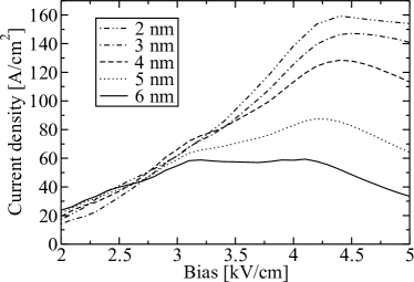
(a)

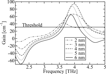
(b)

Figure 2: LABEL:sub@subfig:BTC-6wells-barrier-current Simulated current density and LABEL:sub@subfig:BTC-6wells-barrier-gain gain spectra of optimized BTC QCLs for different injection barrier thicknesses. An indicative figure for the lasing threshold is included for reference, based on calculations of the waveguide losses in Ref. Thesis_Valavanis2009, .

The thickness of the injection barrier is known to be an important parameter in III–V THz QCLs as it can significantly affect the performance of devices.Elec_Lett_Luo_2007 If the injection barrier is too thin, selectivity of injection into the upper laser level is poor; if it is too thick, the tunneling rate through the barrier is small and efficient injection cannot be achieved. Semiclassical rate-equation models of charge injection in THz QCLs lack sensitivity to the injection barrier thickness, and a model that accounts for coherent effects is therefore required.JAPCallebaut2005 Here, we systematically vary the thickness of the injection barrier in the design template, and use our DM simulation to determine the gain and current density. We use the genetic algorithm described in Ref. Ko2010, to maximize the simulated gain of the device at 4 THz by varying the thickness of each of the other layers in the structure, and the applied electric field.

In all the cases considered here, the optimized layer widths (excluding the injection barrier) were found to be identical (to ångström precision) to those of the template. This can be understood by recalling that the decoupled wavefunctions in the DM model are found by embedding the active-region module between thick barriers. Therefore, the layer-width optimization procedure only directly affects the single-period Hamiltonian, and has a very much weaker influence on the interperiod coupling (by slightly adjusting the Rabi frequencies). As such, the results below can be seen to solely represent the effect of the injection barrier thickness upon the device performance without including any contribution from changes in the bandstructure within the period.

Figure 2a shows the simulated current density as a function of applied electric field for optimized devices with 2, 3, 4, 5, and 6-nm-thick injection barriers. Interperiod scattering between spatially-extended wavefunctions is avoided in the DM model, and the simulated current density is therefore a smoothly-varying function of bias in all cases. The alignment bias for the device is approximately 4 kV/cm for all five structures, and we see that the current density at this bias decreases monotonically as the thickness of the injection barrier increases. The gain spectrum for each structure at the alignment bias is shown in Fig. 2b. The variation in the magnitude of the peak gain with injection barrier thickness is not monotonic, and there is an optimum thickness at around 4–5 nm, at which a gain of around 90 cm^-1 is predicted. The difference in gain spectrum between the device with 2-nm-thick injection barriers and the other structures is caused principally by the reduction of injection selectivity into the ULL. It is important to note, however, that the “injection barrier” in this structure is thinner than the 2.5-nm-thick barrier at the end of the module, and the chosen subdivision of modules for tunneling transport in the DM model is likely to be unrealistic.

(a)

(b)

Figure 3: Bandstructure of the six-well BTC QCLs with interdiffusion lengths of LABEL:sub@subfig:BTC-6well-diff1 $L_{d}=1$ nm and LABEL:sub@subfig:BTC-6well-diff2 $L_{d}=2$ nm.

III.2 Interdiffusion compensation

Epitaxial Ge/SiGe heterostructures have been reported to show significant interdiffusion between the pure and alloy semiconductor layers, with typical characteristic interdiffusion lengths estimated to be of the order of 1–2 nm.IEEELever2010 ; OptLettLever2011 This leads to significant changes in the bandstructure and scattering lifetimes,PRBValavanis2008 ; JOAValavanis2009 and can therefore degrade the performance of devices. In this section, we investigate the impact of interdiffusion on the QCL gain and we attempt to recover the lost performance through design optimization.

We account for the effects of interdiffusion by applying a Gaussian annealing model to the alloy composition profile,IEEELi1996 such that the alloy fraction across the interface is described by a Gauss error function with the interdiffusion length $L_{d}$ as a size parameter. Figure 3 shows the bandstructure of the QCL design template with 1 and 2 nm interdiffusion included. The interdiffusion causes the barriers to become reduced in height and the shape of the quantum wells becomes distorted, with the tops being widened and the bottoms being narrowed. For interdiffusion lengths of 2 nm, the thinner barriers near the optically active wells are significantly reduced in height and the ULL is poorly confined.

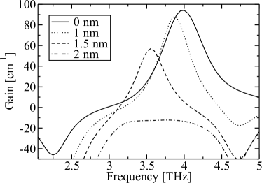
(a)

(b)

Figure 4: Simulated gain of the QCL for interdiffusion lengths of 1, 1.5 and 2 nm; LABEL:sub@subfig:BTC-6well-diff-no-opt without optimization and LABEL:sub@subfig:BTC-6well-diff-opt where the device structure was optimized. In each case, the legend of the plot indicates the interdiffusion length.

Fig. 4a shows the simulated gain spectra for structures with $L_{d}$ in the range 0–2 nm at the respective operating bias for each device. Here, the interdiffusion has been included without subsequently optimizing the design. There is no significant drop in the peak gain when 1 nm interdiffusion length is included. However, for larger interdiffusion lengths the simulated peak gain is reduced considerably, and there is no simulated gain at all for the structure with $L_{d}=2$ nm.

We applied the design optimization algorithm to each of the diffuse QCL structures, and the resulting gain spectra are shown in Fig. 4b. It can be seen that the gain has been fully recovered for structures with interdiffusion lengths up to 1.5 nm. This highlights the importance of being able to characterize the interdiffusion length in these system: so long as this is known, and so long as it is 1.5 nm or less, our results indicate that it can be taken into account in the design process.

For interdiffusion lengths of 2 nm or more, the gain cannot be recovered. There are two reasons for this: first, the ULL is no longer confined by the thin barriers in the structure, which leads to a large spatial overlap with the miniband states, and hence a loss of population inversion. Second, the interdiffusion introduces Si into the nominally pure Ge well regions, leading to a large increase in alloy disorder scattering rates.PRBValavanis2008 As such, additional rapid scattering pathways are introduced to the system, leading to rapid depopulation of the ULL. By way of comparison, we have previously shown that the total scattering rate within a Si/Ge/Si quantum well increases by 50% at an interdiffusion length of 1.21 nm.JOAValavanis2009

IV Conclusion

We have investigated coherent transport effects in a Si-based THz QCL through the use of an extended density matrix model that includes in its basis all subbands that are involved in interperiod transport. Our use of the non-rotating wave approximation allows a steady-state solution to the Liouville equation without a priori knowledge of the bandstructure of the device. In all cases, the non-RWA solution yielded a single strongly-dominant frequency component in each density term, indicating that it would be in good agreement with an equivalent RWA model. Although we have used our generalised non-RWA model to analyze coherent effects in Si-based QCLs, it is equally applicable to III–V QCL structures.

We have coupled our model with a semi-automated QCL design algorithm, and have shown that the optimum injection barrier thickness for Si-based BTC THz QCL structures is in the range 4–5 nm, and we predict peak gain values of $\sim 90$ cm^-1 at a lattice temperature of 4 K. We have also studied the effect of interdiffusion between the Ge and GeSi layers, and found that it is possible to compensate for interdiffusion effects through design optimization up to a limit of $L_{d}\approx 1.5$ nm.

- (1) R. Köhler, A. Tredicucci, F. Beltram, H. E. Beere, E. H. Linfield, A. G. Davies, D. A. Ritchie, R. C. Iotti, and F. Rossi, Nature 417, 156 (2002)
- (2) A. W. M. Lee, Q. Qin, S. Kumar, B. S. Williams, Q. Hu, and J. L. Reno, Appl. Phys. Lett. 89, 141125 (2006)
- (3) S. Fathololoumi, E. Dupont, C. Chan, Z. Wasilewski, S. Laframboise, D. Ban, A. Matyas, C. Jirauschek, Q. Hu, and H. C. Liu, Opt. Express 20, 3866 (2012)
- (4) G. Dehlinger, L. Diehl, U. Gennser, H. Sigg, J. Faist, K. Ensslin, D. Grützmacher, and E. Müller, Science 290, 2277 (2000)
- (5) S. A. Lynch, R. Bates, D. J. Paul, D. J. Norris, A. G. Cullis, Z. Ikonić, R. W. Kelsall, P. Harrison, D. D. Arnone, and C. R. Pidgeon, Appl. Phys. Lett. 81, 1543 (2002)
- (6) A. Valavanis, T. V. Dinh, L. J. M. Lever, Z. Ikonić, and R. W. Kelsall, Phys. Rev. B 83, 195321 (2011)
- (7) L. Lever, A. Valavanis, C. A. Evans, Z. Ikonić, and R. W. Kelsall, Appl. Phys. Lett. 95, 131103 (2009)
- (8) K. Driscoll and R. Paiella, Appl. Phys. Lett. 89, 191110 (2006)
- (9) R. W. Kelsall and R. A. Soref, Int. J. High Speed Electron. 13, 547 (2003)
- (10) A. Valavanis, L. Lever, C. A. Evans, Z. Ikonić, and R. W. Kelsall, Phys. Rev. B 78, 035420 (2008)
- (11) L. Lever, A. Valavanis, Z. Ikonić, and R. W. Kelsall, Appl. Phys. Lett. 92, 021124 (2008)
- (12) K. Driscoll and R. Paiella, J. Appl. Phys. 102, 093103 (2007)
- (13) G. Sun, H. H. Cheng, J. Menéndez, J. B. Khurgin, and R. A. Soref, Appl. Phys. Lett. 90, 251105 (2007)
- (14) V. D. Jovanović, S. Höfling, D. Indjin, N. Vukmirović, Z. Ikonić, P. Harrison, J. P. Reithmaier, and A. Forchel, J. Appl. Phys. 99, 103106 (2006)
- (15) H. Callebaut and Q. Hu, J. Appl. Phys. 98, 104505 (2005)
- (16) J. B. Khurgin, Y. Dikmelik, P. Q. Liu, A. J. Hoffman, M. D. Escarra, K. J. Franz, and C. F. Gmachl, Appl. Phys. Lett. 94, 091101 (2009)
- (17) S. Kumar and Q. Hu, Phys. Rev. B 80, 245316 (2009)
- (18) E. Dupont, S. Fathololoumi, and H. C. Liu, Phys. Rev. B 81, 205311 (2010)
- (19) R. Terazzi and J. Faist, New J. Phys. 12, 033045 (2010)
- (20) M. A. Talukder, J. Appl. Phys. 109, 033104 (2011)
- (21) M. A. Talukder and C. R. Menyuk, New J. Phys. 13, 083027 (2011)
- (22) A. Wacker, Phys. Rev. B 66, 085326 (2002)
- (23) T. Kubis, C. Yeh, and P. Vogl, J. Comp. Electron. 7, 432 (2008)
- (24) T. Kubis, C. Yeh, P. Vogl, A. Benz, G. Fasching, and C. Deutsch, Phys. Rev. B 79, 195323 (2009)
- (25) H. Yasuda, T. Kubis, P. Vogl, N. Sekine, I. Hosako, and K. Hirakawa, Appl. Phys. Lett. 94, 151109 (2009)
- (26) I. Savić, N. Vukmirović, Z. Ikonić, D. Indjin, R. W. Kelsall, P. Harrison, and V. Milanović, Phys. Rev. B 76, 165310 (2007)
- (27) C. Weber, A. Wacker, and A. Knorr, Phys. Rev. B 79, 165322 (2009)
- (28) Y. H. Ko and J. S. Yu, Phys. Status Solidi A 207, 2190 (2010)
- (29) H. Luo, S. R. Laframboise, Z. R. Wasilewski, and H. C. Liu, Electron. Lett. 43, 633 (2007)
- (30) C. G. Van de Walle and R. M. Martin, Phys. Rev. B 34, 5621 (1986)
- (31) A. Valavanis, Z. Ikonić, and R. W. Kelsall, Phys. Rev. B 75, 205332 (2007)
- (32) M. Virgilio and G. Grosso, Phys. Rev. B 79, 165310 (2009)
- (33) A. Yariv, C. Lindsey, and U. Sivan, J. Appl. Phys. 58, 3669 (1985)
- (34) L. W. Casperson, Phys. Rev. A 46, 401 (1992)
- (35) D.-W. Wang, A.-J. Li, L.-G. Wang, S.-Y. Zhu, and M. S. Zubairy, Phys. Rev. A 80, 063826 (2009)
- (36) L. Gil and G. L. Lippi, Phys. Rev. A 83, 043840 (2011)
- (37) G. Beji, Z. Ikonić, C. A. Evans, D. Indjin, and P. Harrison, J. Appl. Phys. 109, 013111 (2011)
- (38) B. Rössner, D. Chrastina, G. Isella, and H. Von Känel, Appl. Phys. Lett. 84, 3058 (2004)
- (39) M. Bonfanti, E. Grilli, M. Guzzi, M. Virgilio, G. Grosso, D. Chrastina, G. Isella, H. von Känel, and A. Neels, Phys. Rev. B 78, 041407 (2008)
- (40) V. A. Shah, A. Dobbie, M. Myronov, D. J. F. Fulgoni, L. J. Nash, and D. R. Leadley, Appl. Phys. Lett. 93, 192103 (2008)
- (41) V. Shah, A. Dobbie, M. Myronov, and D. Leadley, J. Appl. Phys. 107, 064304 (2010)
- (42) P. Harrison, Quantum Wells, Wires and Dots, 2nd ed. (Wiley, Chichester, 2005)
- (43) A. Valavanis, -type silicon-germanium based terahertz quantum cascade lasers, Ph.D. thesis, School of Electronic and Electrical Engineering, University of Leeds (2009), http://etheses.whiterose.ac.uk/1262/
- (44) L. Lever, Z. Ikonić, A. Valavanis, J. D. Cooper, and R. W. Kelsall, J. Lightwave Technol. 28, 3273 (2010)
- (45) L. Lever, Y. Hu, M. Myronov, X. Liu, N. Owens, F. Y. Gardes, I. P. Marko, S. J. Sweeney, Z. Ikonić, D. R. Leadley, G. T. Reed, and R. W. Kelsall, Opt. Lett. 36, 4158 (2011)
- (46) A. Valavanis, Z. Ikonić, and R. W. Kelsall, Phys. Rev. B 77, 075312 (2008)
- (47) A. Valavanis, Z. Ikonić, and R. W. Kelsall, J. Opt. A 11, 054012 (2009)
- (48) E. H. Li, B. L. Weiss, and K.-S. Chan, IEEE J. Quantum Electron. 32, 1399 (1996)