Properties of nano-islands formation in nonequilibrium reaction-diffusion systems with memory effects

Abstract

We study dynamics of pattern formation in systems belonging to class of reaction-Cattaneo models including persistent diffusion (memory effects of the diffusion flux). It was shown that due to the memory effects pattern seletion process are realized. We have found that oscillatory behavior of the radius of the adsorbate islands is governed by finite propagation speed. It is shown that stabilization of nano-patterns in such models is possible only by nonequilibrium chemical reactions. Oscillatory dynamics of pattern formation is studied in details by numerical simulations.

I Introduction

From theoretical and experimental observations it is known that reaction-diffusion systems play an important role in the study of generic spatiotemporal behavior of nonequilibrium systems. Usually such models admit main contributions related to both local dynamics (chemical reactions type of birth-and-death processes) and mass transport. Novel experimental methods, such as field ion microscopy, scanning tunneling microscopy can be used to monitor chemical reactions on the metal surfaces with atomic resolution.

In adsorption-desorption processes when material can be deposited from the gaseous phase such experimental methods allow one to investigate formation of clusters or islands of adsorbed molecules/atoms ZTWE96 . Such islands can have linear size of nanometer range GLRBE94 . In Refs.KNSZGC91 ; PWCL97 ; BGBK98 ; CF99 ; Nature99 it was experimentally shown that nano-patterns on solid surface and nano-islands in adsorbed mono-atomic layers can be organized. It was found that patterns on scales shorter than the diffusion length emerge from the interplay of reactions and lateral interactions between adsorbed particles. The adsorbate presence can modify the local crystallographic structures of the substrate’s surface layer producing long range interactions between adsorbed atoms and their clusters (see for example, Refs.ZKRGL94 ; M91 ; V92 ). It was observed experimentally that nanometer-sized vacancy islands can be organized in a perfect triangular lattice when a single monolayer of Ag was exposed on Ru(0001) surface at room temperature Nature99 . Nanometer elongated islands was observed experimentally in Si/Si(100) 202 , the same was found at deposition of Ge on Si sem2002 , metallic elongated islands were observed at deposition of Cu on Pd(110) 206 . It was shown that elongated adsorbate clusters are governed by formation of dimers and their reconstructions MBE1998 representing nonequilibrium chemical reactions.

It is well known that short-range transient patterns can be observed at initial stages of phase separation processes Binder . These transient patterns can be stabilized by nonequilibrium chemical reactions leading to emergence of stationary patterns TH96 . In models of systems with adsorption and desorption processes additional chemical reactions should be introduced to freeze the patterns. It was shown previously, that adsorption and thermal desorption are “equilibrium reactions” which can not induce the formation of kinetic spatially modulated stationary phases HM96 ; BHKM97 . A problem of formation of stationary microstructures in such systems with irreversible nonequilibrium chemical reactions was considered in Refs.HME98_1 ; HME98_2 . Properties of pattern formation in systems of adsorption-desorption type with dissipative dynamics were studied previously ME94 ; BHKM97 . Pattern formation in pure dissipative stochastic systems with multiplicative noise obeying fluctuation-dissipation relation was discussed in Refs.MW2005 ; M2010 ; PhysD2009 ; PhysScr2011 . It was shown that such multiplicative noise can sustain stationary patterns of nano-size range in pure dissipative systems.

As far as the reactions are defined through chemical kinetics, an evolution of the field variable, let say coverage for adsorption/desorption systems, is governed by the reaction-diffusion equation. A typical deterministic equation is of the form

$$\partial_{t}x=f(x)-\nabla\cdot\mathbf{J},$$ (1)

where $x=x(\mathbf{r},t)$ is the local coverage at surface defined as the quotient between the number of adsorbed particles in a cell of the surface and the fixed number of available sites in each cell, $x\leq 1$. The term $f(x)$ stands for local dynamics and describes birth-and-death or adsorption-desorption processes; the flux $\mathbf{J}$ represents the mass transport.

Most of the theoretical studies deal with the standard Fick law $\mathbf{J}=-D\nabla x$, where $D$ is the diffusion constant. It is known that at $f=0$ the ordinary diffusion equation $\partial_{t}x=\nabla\cdot D\nabla x$ has the unrealistic feature of infinitely fast (infinite) propagation. In such a case a fundamental solution

$$x(r,t)=(4\pi Dt)^{-1/2}\exp(-r^{2}/Dt)$$

means that for any small $t$ at any large $r$ the quantity $x$ will be nonzero, though exponentially small. It leads to unphysical effect that particles move with infinite speed (more than sound speed in solids). The reason for this is lack of correlations of particle motion. To avoid such pathology the diffusion flux can be generalized by taking into account memory effects JP89

$$\mathbf{J}=-\int\limits_{0}^{t}M(t,t^{\prime})D\nabla x(\mathbf{r},t^{\prime}){\rm d}t^{\prime}$$ (2)

described by the memory kernel $M(t,t^{\prime})=\tau_{J}^{-1}\exp(-|t-t^{\prime}|/\tau_{J})$. The delay time $\tau_{J}$ is related to correlated (persistent) random walk. In the limit $f(x)=0$ one gets the finite propagation speed $\sqrt{D/\tau_{J}}$. At $\tau_{J}\to 0$ the asymptotic $M(t,t^{\prime})=\delta(t-t^{\prime})$ leads to the Fick law $\mathbf{J}=-D\nabla x$ with infinite propagation. As far as real systems (molecules, atoms) have finite propagation speed one should use Eq.(2) or an equivalent equation: $\tau_{J}\partial_{t}\mathbf{J}=-\mathbf{J}-D\nabla x$ H1999 . Equations (1,2) can be combined into the one reaction-Cattaneo equation of the form

$$\tau_{J}\partial^{2}_{tt}x+(1-\tau_{J}f^{\prime}(x))\partial_{t}x=f(x)+\nabla\cdot D\nabla x,$$ (3)

where prime denotes derivative with respect to the argument. In the absence of reaction term $(f=0)$ the corresponding telegraph equation has a solution of the form

$$x(r,t)=\left\{\begin{split}&\frac{1}{N}\exp\left(-\frac{t}{2\tau_{J}}\right)I_{0}\left(\sqrt{\frac{\chi}{N}}\right),\ \ \text{for}~{}~{}|r|<\sqrt{\frac{Dt}{\tau_{J}}},\\ &0\ \ \ \text{otherwise},\end{split}\right.$$

where $N=\sqrt{4D\tau_{J}}$, $\chi=(D/\tau_{J})t^{2}-r^{2}$, $I_{0}(\cdot)$ is the modified Bessel function. As was pointed out in Ref.H1999 this equation has some restrictions: (i) it typically does not preserve positivity of the solution $x(\mathbf{r},t)$; (ii) the damping coefficient must be positive, i.e., $f^{\prime}(x)<\tau_{J}^{-1}$.

Therefore, one can use more realistic model given by Eq.(3), where particles have finite speed at smaller time scales and approach diffusion motion on larger time scales. It follows that depending on the form of the reaction term $f(x)$ Eq.(3) admits oscillatory solutions H1999 . An application of such formalism for phase separation processes study with finite $\tau_{J}$ allows one to describe pattern selection processes at early stages of decomposition in binary systems (see Refs.lzg ; PhysA1_2010 ) and oscillatory formation of the ordered phase in crystalline systems CEJP . Oscillatory solutions in class of reaction-Cattaneo systems with fluctuating quantity $\tau_{J}$ were considered in Ref.Ghosh2010 .

In this study we are aimed to describe dynamics of pattern formation and selection processes in a class of reaction-Cattaneo systems given by Eq.(3). Novelty of our approach is in studying oscillatory dynamics of pattern formation in such class of models with chemical reactions governed by adsorption/desorption processes. Following the formalism proposed in Refs.HME98_2 ; MW2005 ; M2010 we compare a behaviour of ordinary reaction-diffusion dissipative system and reaction-Cattenao system. It will be shown below that for the last class of models pattern selection processes are realized, stable patterns possible only if nonequilibrium chemical reactions are introduced. Studying behavior of islands size as clusters of dense phase we will show that averaged island size behaves itself in oscillatory manner. Considering formation of islands of adsorbed particles we discuss properties of the island size distribution during the system evolution.

The paper is organized as follows. In Section II we propose the stochastic reaction-Cattenao model. The linear stability analysis and properties of pattern selection processes are presented in Section III. We discuss results of numerical simulation in Section IV. Finally, in Section V, we draw conclusions from our study.

II Model

Let us consider a model where only one class of particles is possible. Following Refs.MW2005 ; M2010 ; ME94 ; BHKM97 ; CWM2002 ; HME98_1 ; HME98_2 one assumes that the particles can be adsrobed, desorbed, can diffuse and interact among themselves. Therefore, we introduce the scalar field describing dynamics of the local coverage at surface $x(\mathbf{r},t)\in[0,1]$. The reaction term incorporating adsorption and desorption terms together with nonequilibrium chemical reactions is as follows: $f_{0}(x)=k_{a}p(1-x)-k_{d}x\exp(U(\mathbf{r})/T)-k_{r}x^{n}$. Here $k_{a}$ and $k_{d}$ are adsorption and desorption rates, respectively; $p$ is the partial pressure of the gaseous phase; $U(\mathbf{r})$ is the interaction potential. The last term corresponds to nonequilibrium chemical reaction of the order $n\geq 1$ with the rate constant $k_{r}$. Usually it estimates islands/dimers formation or associative desorption MBE1998 . In further consideration we put $n=2$.

The total flux $\mathbf{J}$ is a sum of both ordinary diffusion flux $(-D_{0}\nabla x)$ and flow of adsorbate $(-(D_{0}/T)x(1-x)\nabla U)$. Here the multiplier $x(1-x)$ denotes that the flux is only possible to the $(1-x)$ free sites. Hence, the total flux is

$$\mathbf{J}=-D_{0}\nabla x-\frac{D_{0}}{T}x(1-x)\nabla U;$$ (4)

in an equivalent form one has

$$\mathbf{J}=-D_{0}M(x)\left[\frac{\nabla x}{x(1-x)}+\frac{1}{T}\nabla U\right],$$ (5)

where the Cahn mobility $M(x)=x(1-x)$ is introduced.

Formally the right hand side of Eq.(5) can be rewritten as follows:

$$\mathbf{J}=-D_{0}M(x)\nabla\frac{\delta\mathcal{F}}{\delta x},$$ (6)

where the total mesoscopic free energy functional is

$$\mathcal{F}=\mathcal{F}_{0}+\mathcal{F}_{int}.$$ (7)

The non-interacting part takes the form

$$\mathcal{F}_{0}=\int{\rm d}\mathbf{r}\left[x(\mathbf{r})\ln(x(\mathbf{r}))+(1-x(\mathbf{r}))\ln(1-x(\mathbf{r}))\right],$$ (8)

whereas $\mathcal{F}_{int}$ is governed by the interaction potential $U$ which we assume in the standard form BHKM97

$$U(\mathbf{r})=-\int{\rm d}\mathbf{r}^{\prime}u(\mathbf{r}-\mathbf{r}^{\prime})x(\mathbf{r}^{\prime}),$$ (9)

where $-u(r)$ is the binary attraction potential for two adsorbate particles separated by the distance $r$, it is of symmetrical form , i.e. $\int{\rm d}\mathbf{r}\mathbf{r}^{2n+1}u(\mathbf{r})=0$, $n=1,\ldots,\infty$.

Therefore, one can rewrite the total mesoscopic free energy as follows:

$$\mathcal{F}=\int{\rm d}\mathbf{r}\left[x\ln(x)+(1-x)\ln(1-x)\right]-\frac{1}{2T}\iint{\rm d}\mathbf{r}{\rm d}\mathbf{r}^{\prime}x(\mathbf{r})u(\mathbf{r}-\mathbf{r}^{\prime})x(\mathbf{r}^{\prime}).$$ (10)

Following Ref.HME98_2 as a simple approximation for the interaction potential, we choose the Gaussian profile

$$u(r)=\frac{2\epsilon}{\sqrt{4\pi r_{0}^{2}}}\exp(-r^{2}/4r_{0}^{2}),$$ (11)

where $\epsilon$ is the interaction strength, $r_{0}$ is the interaction radius. Assuming that $x$ does not vary significantly within the interaction radius, one can estimate

$$\int{\rm d}\mathbf{r}^{\prime}u(\mathbf{r}-\mathbf{r}^{\prime})x(\mathbf{r}^{\prime})\simeq\int{\rm d}\mathbf{r}^{\prime}u(\mathbf{r}-\mathbf{r}^{\prime})\sum_{n}\frac{(\mathbf{r}-\mathbf{r}^{\prime})^{n}}{n!}\nabla^{n}x(\mathbf{r}).$$ (12)

Substituting Eq.(11) into Eq.(12) up to terms of the 4-th order one gets $\int u(r)x(r){\rm d}r=2\epsilon x$, $\frac{1}{2!}\int u(r)r^{2}\nabla^{2}x(r){\rm d}r=2\epsilon r_{0}^{2}\nabla^{2}x$, $\frac{1}{4!}\int u(r)r^{4}\nabla^{4}x(r){\rm d}r=\epsilon r_{0}^{4}\nabla^{4}x$.

Therefore, using notation $\varepsilon=\epsilon/T$ one has

$$\frac{1}{T}\int{\rm d}\mathbf{r}^{\prime}u(\mathbf{r}-\mathbf{r}^{\prime})x(\mathbf{r}^{\prime})\simeq\varepsilon x(\mathbf{r})+\varepsilon(1+r_{0}^{2}\nabla^{2})^{2}x(\mathbf{r}).$$ (13)

The total free energy functional takes the form

$$\mathcal{F}=\int{\rm d}\mathbf{r}\left[-\frac{\varepsilon}{2}x^{2}+x\ln x+(1-x)\ln(1-x)-\frac{\varepsilon}{2}x(1+r_{0}^{2}\nabla^{2})^{2}x\right].$$ (14)

Therefore, the total flux can be written as

$$\mathbf{J}=-D_{0}M(x)\nabla\left[\frac{\delta\mathcal{F}_{loc}}{\delta x}-\varepsilon(1+r_{0}^{2}\nabla^{2})^{2}x\right],$$ (15)

here $\mathcal{F}_{loc}$ is defined through the local part of the free energy density (first three terms in Eq.(14)).

Next, it will be more convenient to measure time in units $k_{d}$, introduce the diffusion length $L_{d}=\sqrt{D_{0}/k_{d}}$ and dimensionless adsorption rates $\alpha=k_{a}p/k_{d}$, $\beta=k_{r}/k_{d}$. Therefore, the reaction term takes the form $f(x)=\alpha(1-x)-xe^{-2\varepsilon x}-\beta x^{2}$ and the system is described by two length scales, where $r_{0}\ll L_{d}$. As far as real systems (molecules, atoms) have finite propagation speed one should take into account memory (correlation) effects, assuming

$$\mathbf{J}=-L_{d}\int\limits_{0}^{t}{\rm d}t^{\prime}\mathcal{M}(t,t^{\prime};\tau_{J})\nabla\frac{\delta\mathcal{F}}{\delta x(\mathbf{r},t^{\prime})},$$ (16)

where $\mathcal{M}(t,t^{\prime})$ is the memory kernel. Taking it in the exponential decaying form $\mathcal{M}(t,t^{\prime})=\tau_{J}^{-1}M(x(\mathbf{r},t^{\prime}))\exp(-|t-t^{\prime}|/\tau_{J})$, where $\tau_{J}$ is the flux relaxation time instead of one equation for the coverage we get a system of two equations:

$$\begin{split}\partial_{t}&x=f(x)-L_{d}\nabla\cdot\mathbf{J};\\ \tau\partial_{t}&\mathbf{J}=-\mathbf{J}-L_{d}M(x)\nabla\frac{\delta\mathcal{F}}{\delta x},\quad\tau=\tau_{J}k_{d}.\end{split}$$ (17)

At $\tau_{J}\to 0$ the asymptotic $M(t,t^{\prime})=\delta(t-t^{\prime})$ leads to the Fick law $\mathbf{J}=-L_{d}M(x)\nabla{\delta\mathcal{F}_{tot}}/{\delta x}$ with an infinite propagation.

The equivalent equation for the coverage takes the form

$$\begin{split}&\tau\partial^{2}_{tt}x+\gamma(x)\partial_{t}x=\varphi(x,\nabla),\quad\gamma(x)\equiv 1-\tau f^{\prime}(x);\\ &\varphi(x;\nabla)\equiv f(x)+L_{d}^{2}\nabla\cdot[\nabla x-\varepsilon M(x)(\nabla x+\nabla\mathcal{L}_{SH}x)],\quad\mathcal{L}_{SH}=(1+r_{0}^{2}\nabla^{2})^{2}.\end{split}$$ (18)

Let us consider stationary homogeneous system states. In the deterministic limit in the absence of reaction, the system undergoes first order phase transition, where its stationary uniform states are given by $\alpha(1-x)=x\exp(-2\varepsilon x)$. The critical point of this equilibrium phase transition $x_{c}=1/2$ is located at $\varepsilon_{c}=2$ and $\alpha_{c}=\exp(-2)$. A coexistence line of diluted $(x<1/2)$ and dense $(x>1/2)$ phases is given by the relation $\alpha=\exp(-\varepsilon)$. Introduction of the chemical reactions governed by the rate $\beta$ shifts the whole phase diagram and shrinks the domain where the system is bistable. Here possible values for $x$ related to the uniform states decreases whereas critical values for $\varepsilon$ become larger; if $\beta$ grows then critical values for $\alpha$ decrease. The corresponding phase diagram is shown in Fig.1. Outside the cusp the system is monostable: at small $\alpha$ (before the cusp) the system is in low density state $x_{LD}$, whereas at large $\alpha$ the high density state $x_{HD}$ is realized. In the cusp the system is bistable. Critical points and the related coverage are shown in Fig.1b. Here starting from the fixed value for $\beta$ and moving up to an intersection with the curve $\varepsilon^{*}(\beta)$, one gets the critical value $\varepsilon^{*}$ as the corresponding ordinate in the left axis. Than, we move to the right hand side to an intersection with the curve $\varepsilon^{*}(\alpha^{*})$; the corresponding abscissa in the top correspond to critical value $\alpha^{*}$. Moving from this point to an intersection the curve $x^{*}(\alpha^{*})$, one gets the critical value $x^{*}$ as the corresponding ordinate in the right axis. Acting in such a manner, we obtain all needed critical values for the system parameters. Analytical relation between $\alpha^{*}$, $\varepsilon^{*}$, $x^{*}$ and $\beta$ are as follows: $\varepsilon^{*}=(1+\sqrt{5-2x^{*}})/(2x^{*}(2-x^{*}))$, $\alpha^{*}=2\varepsilon^{*2}x^{*3}\exp(-2\varepsilon^{*}x^{*})$, $\beta=2\varepsilon^{*}(1-\varepsilon^{*}x^{*})\exp(-2\varepsilon^{*}x^{*})$.

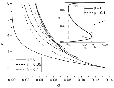
a) b)

Figure 1: Phase diagram for homogeneous system in the parameter plane $(\alpha,\varepsilon)$ (a). Dependencies $x(\alpha)$ in insertion are obtained at $\varepsilon=4$. Critical points located at $\varepsilon^{*}$ and $\alpha^{*}$, and the corresponding coverage $x^{*}$ are shown in plot(b)

III Linear stability analysis

It is known that systems with memory effects admit pattern selection processes at fixed set of the system parameters lzg ; PhysA1_2010 ; CEJP . These processes can be observed at early stages of the system evolution where linear effects are essential. Therefore, pattern selection can be studied considering stability of statistical moments, reduced to the averaged filed and/or structure function as the Fourier transform of a two-point correlation function for the coverage. As far as fourth order contribution in the interaction potential $u(r)$ is not essential at small $r_{0}\ll L_{d}$, next we consider a case where $\int u(r)x(r){\rm d}r\simeq 2\varepsilon(1+r_{0}^{2}\nabla^{2})x$, neglecting $r_{0}^{4}\nabla^{4}x$.

Averaging Eq.(18) over initial conditions and taking $\langle x\rangle-x_{0}\propto e^{{\rm i}(\omega t-kr)}$ one gets the dispersion relation of the form

$$\omega(k)_{\mp}=-\frac{{\rm i}\gamma(x_{0})}{2\tau}\mp\left[\frac{L_{d}^{2}k^{2}(1-2\varepsilon M(x_{0})(1-r_{0}^{2}k^{2}))-f^{\prime}(x_{0})}{\tau}-\frac{\gamma^{2}(x_{0})}{4\tau^{2}}\right]^{1/2}.$$ (19)

One can see that $\omega(k)$ can have real and imaginary parts, i.e. $\omega(k)=\Re\omega(k)\pm{\rm i}\Im\omega(k)$. The component $\Re\omega(k)$ is responsible for oscillatory solutions, whereas $\Im\omega(k)$ describes stability of the solution $\langle\delta x_{\mathbf{k}}(\omega)\rangle$. Analysis of both $\Re\omega(k)$ and $\Im\omega(k)$ allows us to set a threshold for a wave-number where oscillatory solutions are possible. Moreover, it gives a wave-number for the first unstable solution. From the obtained dispersion relations it follows that at $k=k_{0}$ satisfying equation

$$k_{0}^{2}(1-2\varepsilon M(x_{0})(1-r_{0}^{2}k_{0}^{2}))=\frac{1}{L_{d}^{2}}\left[f^{\prime}(x_{0})+\frac{\gamma^{2}(x_{0})}{4\tau}\right]$$ (20)

two branches of the dispersion relation degenerate. The unstable mode appears at $k=k_{c}$ obtained from the equation

$$L_{d}^{2}k_{c}^{2}(1-2\varepsilon M(x_{0})(1-r_{0}^{2}k_{c}^{2}))=f^{\prime}(x_{0}).$$ (21)

From the dispersion relation $\omega(k)$ one can find the most unstable mode $k_{m}$ as a solution of the equation ${\rm d}\Im\omega/{\rm d}k=0$. It coincides with first unstable mode when only one nonzeroth solution of the equation $\Im\omega(k)=0$ emerges.

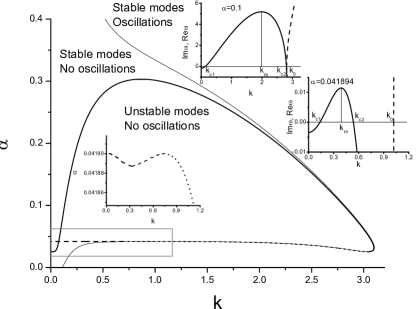
Figure 2: Stability diagram at $\varepsilon=5$, $\tau=0.5$, and $\beta=0.1$. Dependencies of $\Im\omega(k)$ and $\Re\omega(k)$ are shown as solid and dashed lines in insertions at $\alpha=0.1$ and $\alpha=0.041894$ related to high density and low density phases

Using obtained relations one can calculate a diagram indicating spatial stability of all homogeneous states to inhomogeneouse perturbations. The corresponding diagram is shown in Fig.2. Here domain of unstable modes with respect to inhomogeneous perturbations is limited by solid and dashed thick curves. The solid curve relates to high density phase, whereas dashed line corresponds to low density phase; dotted line addresses to unstable homogeneous stationary state. When we increase the adsorption rate $\alpha$ from zeroth value the first unstable mode emerges at large $k$ and is possible only for high density phase. There is small domain for $\alpha$ where spatial instability of the low density phase is possible (see magnified insertion of $\alpha(k)$ at small $\alpha$ and $k$). It is should be noted that wave numbers related to these unstable modes in both low- and high density phases are observed in fixed interval $k\in[k_{c1},k_{c2}]$. The thin solid line in Fig.2 denotes critical values $k_{o}$ where oscillatory solutions $\langle x(k,t)\rangle$ are possible. The domain of unstable modes with respect to inhomogeneous perturbations is limited by large values for $\alpha$. It means that instability of high density phase is possible only in fixed interval for adsorption rate values.

According to obtained dependencies $\alpha(k)$ we plot in Fig.3 critical values for $\alpha$ and $\varepsilon$ related to formation of spatially modulated phases, where solid lines denote binodals, dashed lines bound spatially modulated phases.

a) b)

Figure 3: Critical values for $\varepsilon$ and $\alpha$ related to pattern formation: a) $\beta=0.05$; b) $\beta=0.1$

In the case of $\beta=0$ one has only binodals bounding domains of one uniform phase and domain of two uniform phase existence. Here no spatially modulated phases are possible. When we put $\beta\neq 0$ and increase the adsorption rate at small $\alpha$ only uniform low density state (uLD) is possible; at large $\alpha$ one has only uniform high density state (uHD). In the cusp depending on the values for $\alpha$ one has: uniform low density state and modulated high density phase (uLD& mHD) at small $\alpha$; modulated low density and high density phases (mLD& mHD) at elevated $\alpha$. If we further increase the adsorption rate only modulated high density phase (mHD) is possible. Controlling the rate $\beta$ one can govern size of the domain where both modulated low density and high density phases emerge; when $\beta$ grows the domain of the modulated high density phase increases and mHD phase can emerge before the first binodal (at smaller $\alpha=\alpha_{b1}$).

Considering properties of pattern selection we need to find dynamical equation for the structure function $S(\mathbf{k},t)$ as the Fourier transform of the two-point correlation function $\langle\delta x(\mathbf{r},t)\delta x(\mathbf{r}^{\prime},t)\rangle$ and study its behavior at small times. To that end we obtain the linearized evolution equation for the Fourier components $\delta x_{\mathbf{k}}(t)$ and $\delta x_{-\mathbf{k}}(t)$ and compute $S(\mathbf{k},t)=\langle\delta x_{\mathbf{k}}(t)\delta x_{-\mathbf{k}}(t)\rangle$. The corresponding dynamical equation takes the form

$$\tau\partial^{2}_{tt}S(\mathbf{k},t)+\gamma(x_{0})\partial_{t}S(\mathbf{k},t)=2\left\{f^{\prime}(x_{0})-L_{d}^{2}k^{2}(1-2\varepsilon M(x_{0})(1-r_{0}^{2}k^{2}))\right\}S(\mathbf{k},t).$$ (22)

Analytical solution can be found assuming $S(\mathbf{k},t)-S_{0}\propto\exp(-i\varpi(\mathbf{k})t)$, where

$$\varpi(k)_{\pm}=-\frac{{\rm i}\gamma(x_{0})}{2\tau}\pm\left[\frac{2\left(L_{d}^{2}k^{2}(1-2\varepsilon M(x_{0})(1-r_{0}^{2}k^{2}))-f^{\prime}(x_{0})\right)}{\tau}-\frac{\gamma^{2}(x_{0})}{4\tau^{2}}\right]^{1/2}.$$ (23)

As in the previous case $\Im\varpi$ is responsible for stability of the system, whereas $\Re\varpi$ relates to pattern selection processes.

IV Numerical simulations

A morphology of emergent patterns and dynamics of pattern formation we study by numerical simulations in two dimensional system with $256\times 256$ sites and periodic boundary conditions. In our simulations we take time step $\Delta t=2.5\times 10^{-4}$ and consider the case when $L_{d}=40r_{0}$. The total size of the system is $L=12.8L_{d}$. As initial conditions we take: $\langle x(\mathbf{r},0)\rangle=0$, $\langle(\delta x(\mathbf{r},0))^{2}\rangle=0.1$ where $x(\mathbf{r},t)\in[0,1]$.

Typical evolution of the system with different values for $\tau$, $\varepsilon$ and $\alpha$ at $\beta=0.1$ is shown in Fig.4. In the case of pure dissipative system ($\tau=0$) at $\alpha=0.1$ the adsorbate is organized into separated islands with small difference in the linear sizes of islands. When we put $\tau=0.5$ (see 3-rd column) at the same other system parameters we get pattern where all islands at large time interval are combined into one percolating cluster. Fixing $\tau=0.5$ and taking small $\alpha$ one gets set of adsorbate islands with large difference in their linear sizes (see 2-nd column). With further increase in $\alpha$ islands of vacancies are formed (see 4-th column). Such islands has the same structure as islands of adsorbate at small adsorption rate.

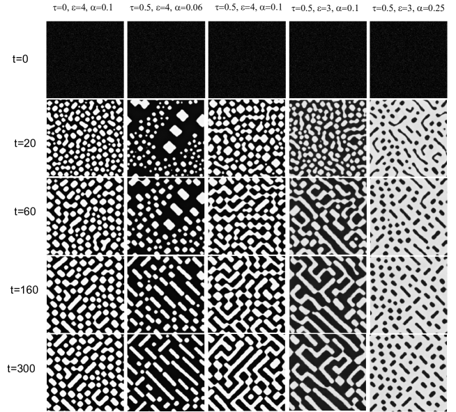
Figure 4: Snapshots of the system evolution at $\beta=0.1$. All snapshots are taken at $t=0$, $t=20$, $t=60$, $t=160$, $t=300$. Here concentration of adatoms is shown with the help of gray scale: white domains correspond to adatoms present, dark ones indicate regions without adatoms.

In Figure 5 we present dynamics of the averaged concentration field $\langle x\rangle$ and its dispersion $\langle(\delta x)^{2}\rangle$. It is known that the growth of the quantity $\langle(\delta x)^{2}\rangle$ means ordering of the system (an increase in fluctuations of the concentration). Following the obtained dependencies one can find that if nonequilibrium reactions are absent ($\beta=0$) the system passes toward an equilibrium thermodynamic state where no stationary patterns can be realized. Here all possible patterns appeared during the system evolution are transient and at final stages the system is totally homogeneous. According to the behavior of both $\langle x\rangle$ and $\langle(\delta x)^{2}\rangle$ one can say that the average goes toward uniform stationary value $x_{0}=x_{HD}$, whereas the dispersion increases at early stages (formation of transient patterns) and after it decreases toward zeroth values (no dispersion in adatoms concentration field is realized). Therefore, the systems moves into homogeneous state. The situation is crucially changed when the nonequilibrium chemical reactions are introduced. Here such reactions freeze patterns formed at coarsening stage, and patterns develop very slowly. As a results of competing between chemical reactions and potential interactions between atoms such patterns are stable in time and can be considered as stationary ones (see Fig.4). Indeed, here the averaged value $\langle x\rangle$ takes lower values than $x_{0}$ related to $\beta=0$ and

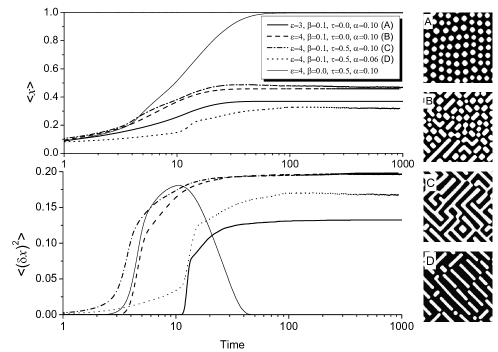
Figure 5: Evolution of $\langle x\rangle$ and $\langle(\delta x)^{2}\rangle$

the dispersion $\langle(\delta x)^{2}\rangle$ does not decrease in time at late stages. Therefore, the quantity $\langle(\delta x)^{2}\rangle$ can be used an effective order parameter. Indeed, if it decreases in time toward zero, then the system moves into homogeneous state, whereas nonzeroth values for the dispersion mean that modulated spatial patterns are realized. From Fig.5 one can see that at $\beta\neq 0$ at large adsorption rate $\alpha$ the system is in the high density state, whereas at elevated interaction strength of the adsorbate small islands of the dense phase are possible; here due to large interactions between adsorbate the evaporation/dissolution processes are less probable. Comparing curves related to two cases $\tau=0$ and $\tau\neq 0$ one can find that in the last case both $\langle x\rangle$ and $\langle(\delta x)^{2}\rangle$ exhibit nonmonotonic behavior, here oscillations with small amplitude are possible. It is well related to results of the linear stability analysis. Moreover, it is interesting to note that in the case $\tau=0$ most of islands of the dense phase are of equiaxial symmetry, whereas at $\tau\neq 0$ such islands are elongated in one of two possible equivalent directions.

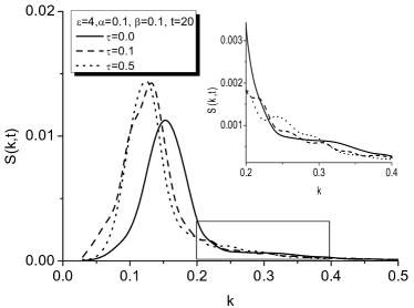
a) b)

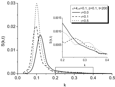
Figure 6: Structure function dynamics for different values of the diffusion flux relaxation time $\tau$ at $t=20$ (a) and $t=200$ (b). Other parameters are: $\alpha=0.1$, $\beta=0.1$, $\varepsilon=4$

Let us consider dynamics of the structure function at different values for $\tau$ and different time intervals (see Fig.6). To calculate $S(k,t)$ we have used fast Fourier transformation procedure. Let us start with the simplest case of $\tau=0$ (see solid lines in Figs.6a,b). Here only major peak of $S(k,t)$ is realized that is related to period of islands. There is smooth behavior of the structure function tails. During the system evolution the peak is shifted toward stationary value of the island size; its height increases (islands become well defined and boundaries between dense and diluted phases become less diffusive). In the case

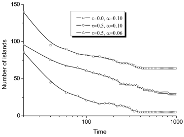
a) b)
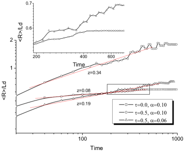
c)

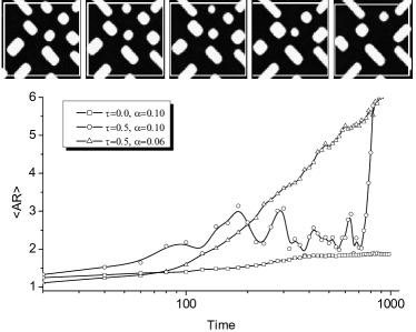
Figure 7: Dynamics of the number of islands (a), averaged island size (b) and the corresponding averaged aspect ratio (c) at $\beta=0.1$. Values for the dynamical exponent $z$ related to the scaling law $\langle R\rangle\propto t^{z}$ are shown near the approximate lines. In plot (c) snapshot of pieces of the system obtained at $t=200$, 220, 240, 280, 300 illustrate a change of $R_{x}/R_{y}$; other parameters are: $\varepsilon=4$, $\beta=0.1$, $\alpha=0.1$.

$\tau\neq 0$ we get one major peak at small wave number and additional peaks at large $k$. Emergence of such minor peaks means formation of other patterns (patterns with other periods). In the course of time an amplitude of such satellite peaks decreases that means pattern selection processes when the system selects one most unstable mode characterized by the major peak whose height increases. This oscillatory behavior of the structure function at large wave numbers is well predicted by the linear stability analysis.

Next, let us study a behavior of the averaged radius of islands. In our computations we have calculated number of sites related to one island. This number corresponds to a square of the island. Assuming that an island with spherical symmetry has the same square we have computed the radius $\langle R\rangle$ of the corresponding spherical island. In Fig.7a we plot dynamics of the number of islands at different values for $\tau$, $\varepsilon$ and $\alpha$. Dynamics of the quantity $\langle R\rangle$ (measured in units of diffusion length $L_{d}$) is shown in Fig.7b. It follows that the system attains the stationary state with finite number of islands. Comparing curves related to different $\tau$, one can find that nonequilibrium effects related to $\tau\neq 0$ decrease essentially the number of islands (but stationary islands have large size). If the adsoprtion rate $\alpha$ is small, then number of islands is large (they are characterized by small sizes). From Fig.7b it is seen that in the simplest case of pure dissipative system characterized by $\tau=0$ the averaged radius is a monotonically increasing quantity. At large time interval it attains a stationary value and does not changed. It means that the coarsening procedure is finished and we get stationary patterns. It follows that islands of the adsorbate have the averaged length $\langle R\rangle\sim(0.15\div 0.9)L_{d}$. Following Refs.CTT06 ; CTT07 one can estimate $\langle R\rangle$ considering deposition of Al on TiN(100): at room temperature one has the lattice constant $a_{Al}=4.05\times 10^{-10}m$, the pair interaction energy $\epsilon_{0}=-0.22~{}eV$ with the coordination number $Z=4$ gives $r_{0}=Za_{Al}\simeq 1.6\times 10^{-9}m$, the diffusion constant $D=10^{-10}cm^{2}s^{-1}$. Hence the patterns have the size $\langle R\rangle\sim(10\div 60)\times 10^{-9}m$.

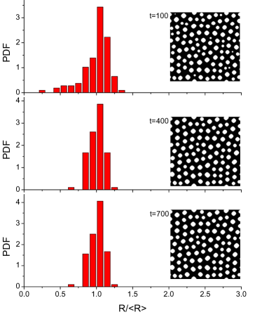
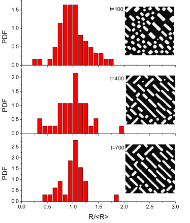
a) b)
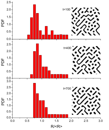
c) d)

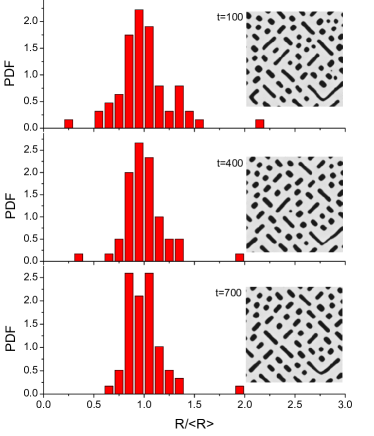
Figure 8: Evolution of the probability density function of the dimensionless radius of the islands size at different $\tau$ at $\beta=0.1$: a) $\tau=0$, $\varepsilon=4$, $\alpha=0.06$; b) $\tau=0$, $\varepsilon=3$, $\alpha=0.25$; c) $\tau=0.5$, $\varepsilon=4$, $\alpha=0.06$; d) $\tau=0.5$, $\varepsilon=3$, $\alpha=0.25$

Studying scaling properties of the island growth we have estimated a scaling exponent $z$ in the islands size growth law $\langle R\rangle\propto t^{z}$. Fitting the data related to stage of growth, we have obtained $z=0.08$ for pure dissipative system with $\varepsilon=4$. Taking $\tau\neq 0$, one can find that at small $\varepsilon$ (in our case $\varepsilon=4$) the averaged radius of islands increases in nonmonotonic manner. Fitting the scaling regime we have found that at $\tau=0.5$ the scaling exponent takes large values, in our case $z=0.34$. When the adsorption rate decreases the growth processes delay and characterize by small dynamical exponent $z$ (at $\alpha=0.06$ one has $z=0.19$). Therefore, nonequilibrium effects related to relaxation of the diffusion flux characterized by $\tau\neq 0$ accelerate growth processes, the same is observed when adsorption rate increases. It is interesting to note that at $\tau\neq 0$ oscillations predicted for the averaged field and the structure function are possible for the dependence $\langle R(t)\rangle$. It means that islands can change their size during the system evolution in oscillating manner. Amplitude of oscillations is well pronounced for large $\alpha$ and small $\varepsilon$.

To prove that islands can oscillatory change their sizes we compute an averaged aspect ratio $\langle AR\rangle=\langle R_{x}/R_{y}\rangle$, where $R_{x}$ and $R_{y}$ are sizes of an island in $x$- and $y$-direction, respectively. From the obtained dependencies shown in Fig.7c it follows that for pure dissipative system deviations from the straight line are small and may be considered as fluctuations in $R_{x}$ and $R_{x}$ values. At $\tau\neq 0$ and small $\varepsilon$ oscillations in $\langle AR\rangle$ are well pronounced. Such oscillations in lateral and longitudinal sizes of islands mean that at some fixed time interval most of the islands grow in one direction whereas in other direction their size decreases, in next time interval these two directions are changed. When this scenario is repeated one gets an oscillation picture of island size growth. In Fig.7c we present snapshots showing change of the growth orientation during the system evolution.

In our study we are interesting also in a behavior of the probability density functions (PDF) of the island sizes distribution. Let us consider PDF’s for pure dissipative system, initially. As Figs.8a,b shows islands of different sizes formed at initial stages evolves in such manner that the most probable value for $R$ is located around $\langle R\rangle$. Islands of other sizes are possible with small probabilities. In the stationary limit PDF has unique well pronounced peak, small fluctuations of island size distribution are possible and are shown as satellite peaks around major one. In the case of $\tau\neq 0$ (see Figs.8c,d) the hyperbolic transport promotes formation of islands with different sizes. The principle difference comparing to the case of pure dissipative system is in a bimodal form of PDF observed at large times. Here at early stages islands of different sizes are formed, and during the system evolution following the Ostwald ripening mechanism small islands dissolve and large islands reduces their sizes. In such a case two well pronounced major peaks of PDF indicate that there two most probable sizes of islands related to $R>\langle R\rangle$ and $R<\langle R\rangle$.

V Conclusions

We have studied dynamics of islands formation of the adsorbate using generalized approach including persistent motion of particles having finite speed at initial stages and diffusion kinetics at final ones. It was found that stabilization of nano-patterns in such class of reaction-Cattaneo models is achieved by noneqilibrium chemical reactions. It was found that during the system evolution pattern selection processes are realized. We have shown that possible oscillatory regimes for islands formation are realized at finite propagation speed related to nonzero relaxation time for the diffusion flux.

Our results can be used to describe formation of nano-islands at processes of condensation from the gaseous phase. Despite we have considered a general model where relaxation time $\tau_{J}$ for the diffusion flux is small but nonzeroth value, one can say that condensation processes with formation of metallic islands can be described in the limit $\tau_{J}/\omega_{D}^{-1}\lesssim 10^{-3}$ (here $\omega_{D}$ is the Debye frequency), whereas nano-islands formation with $\tau_{J}/\omega_{D}^{-1}\sim 10^{-1}\div 10^{-2}$ is possible for soft matter condensation (semiconductors, polymers, etc.).

References

- (1) T.Zambelli, J.Trost, J.Wintterlin, G.Ertl, Phys.rev.Lett. 79 (1996) 795.
- (2) V.Gorodetskii, J.Lauterbach, H.A.Rotermund, J.H.Block, G.Ertl, Nature 370 (1994) 276.
- (3) K.Kern, H.Niehus, A.Schatz, P.Zeppenfeld, J.George, G.Cosma, Phys.Rev.Lett. 67 (1991) 855.
- (4) T.M.Parker, L.K.Wilson, N.G.Condon, F.M.Leissle, Phys.Rev.B 56 (1997) 6458.
- (5) H.Brune, M.Giovannini, K.Bromann, K.Kern, Nature 394 (1998) 451.
- (6) P.G.Clark, C.M.Friend, J.Chem.Phys. 111 (1999) 6991.
- (7) K.Pohl, M.C.Bartelt, J.de la Figuera, N.C.Bartelt, J.Hrbek, R.Q.Hwang, Nature 397 (1999) 238.
- (8) P.Zepenfeld, M.Krzyzowski, C.Romainczyk, G.Gomsa, M.G.Lagally, Phys.Rev.Lett. 72 (1994) 2737.
- (9) V.I.Marchenko, JETP Lett. 67 (1991) 855.
- (10) D.Vanderbit, Surf.Sci. 268 (1992) L300.
- (11) Y.W.Mo, B.S.Swartzentruber, B.Kariotis, M.B.Webb, M.G.Lagally, Phys.Rev.Lett. 63 (1989) 2393.
- (12) G.E.Cirlin, V.A.Egorov, L.V.Sokolov, P.Werner, Semiconductors 36 (2002) 1294-1298.
- (13) J.P.Bucher, E.Hahn, P.Fernandez, C.Massobrio, K.Kern, Europhys.Lett. 27 (1994) 473.
- (14) Harald Brune, Surf.Sci.Reports 31 (1998) 121-229.
- (15) K.Binder, in: P.Haasen (Eds.), Material Science and Technology: Phase Transformations in Materials, Vol.5, VCH, Weinham, 1990.
- (16) Q.Tran-Cong, A.Harada, Phys.Rev.Lett. 76 (1996) 1162.
- (17) M.Hildebrand, A.S.Mikhailov, J.Phys.Chem. 100 (1996) 19089.
- (18) D.Batogkh, M.Hildebrant, F.Krischer, A.Mikhailov, Phys.Rep. 288 (1997) 435.
- (19) M.Heldebrand, A.S.Mikhailov, G.Ertl, Phys.Rev.Lett. 81 (1998) 2602(4).
- (20) M.Heldebrand, A.S.Mikhailov, G.Ertl, Phys.Rev.E 58 (1998) 5483(11).
- (21) A.Mikhailov, G.Ertl, Chem.Phys.Lett. 238 (1994) 104.
- (22) Sergio E.Mangioni, Horacio S. Wio, Phys.Rev.E. 71 (2005) 056203.
- (23) Sergio E.Mangioni, Physica A 389 (2010) 1799.
- (24) D.O.Kharchenko, S.V.Kokhan, A.V.Dvornichenko, Physica D 238 (2009) 2251.
- (25) Dmitrii O.Kharchenko, Vasyl O.Kharchenko, Irina O.Lysenko, Phys.Scr. 83 (2011) 045802(9)
- (26) D.D.Joseph, L.Preziosi, Rev.Mod.Phys. 61 (1989) 41.
- (27) Werner Horsthemke, Phys.Rev.E 60 (1999) 2651.
- (28) N. Lecoq, H. Zapolsky, P. Galenko, Eur.Phys.Jour.ST. 177 (2009) 165.
- (29) P.K.Galenko, Dmitrii Kharchenko, Irina Lysenko, Physica A 389 (2010) 3443.
- (30) Dmytro Kharchenko, Vasyl Kharchenko, Irina Lysenko, Cent.Eur.J.Phys. 9(3) (2011) 698.
- (31) Pushpita Ghosh, Shrabani Sen, Deb Shankar Ray, Phys.Rev.E 81 (2010) 026205.
- (32) S.B.Casal, H.S.Wio, S.Mangioni, Physica A 311 (2002) 443.
- (33) Sergio E.Mangioni, Roberto R.Deza, Phys.Rev.E 82 (2010) 042101.
- (34) M.G.Clerc, E.Tirapegui, M.Trejo, Phys.Rev.Lett. 97 (2006) 176102.
- (35) M.G.Clerc, E.Tirapegui, M.Trejo, Eur.Phys.J. ST. 146 (2007) 407.
- (36) K.R.Elder, Mark Katakowski, Mikko Haataja, Martin Grant, Phys.Rev.Lett. 88 (2002) 245701.
- (37) K.R.Elder, Martin Grant, Phys.Rev.E 70 (2004) 051605.
- (38) Peter Stafanovich, Mikko Haataja, Nikolas Provatas, Phys.Rev.Lett. 96 (2006) 225504.
- (39) D.Kharchenko, I.Lysenko, V.Kharchenko, Physica A 389 (2010) 3356.