Water structure-forming capabilities are temperature shifted for different models

Abstract

A large number of water models exists for molecular simulations. They differ in the ability to reproduce specific features of real water instead of others, like the correct temperature for the density maximum or the diffusion coefficient. Past analysis mostly concentrated on ensemble quantities, while few data was reported on the different microscopic behavior. Here, we compare seven widely used classical water models (SPC, SPC/E, TIP3P, TIP4P, TIP4P-Ew, TIP4P/2005 and TIP5P) in terms of their local structure-forming capabilities through hydrogen bonds for temperatures ranging from 210 K to 350 K by the introduction of a set of order parameters taking into account the configuration of the second solvation shell. We found that all models share the same structural pattern up to a temperature shift. When this shift is applied, all models overlap onto a master curve. Interestingly, increased stabilization of fully coordinated structures extending to at least two solvation shells is found for models that are able to reproduce the correct position of the density maximum. Our results provide a self-consistent atomic-level structural comparison protocol, which can be of help in elucidating the influence of different water models on protein structure and dynamics.

I Introduction

At the fundamental level, water directly influences several biologically relevant processes including protein folding Levy2006 , protein-protein association Papoian2003 ; Levy2006 ; Hummer2010 ; Ahmad2011 and amyloid aggregation Thirumalai2011 . Surprisingly, relatively simple models with fixed charges and geometry are able to reproduce the phase diagram as well as many of the anomalies of water with good accuracy Abascal2009 ; Aragones2011 . For example, all popular classical water models present a density maximum Vega2005 ; Abascal2005 . However, only those that explicitly included this information in the fitting of the potential are able to correctly reproduce the experimental value located at around 277 K at ambient pressure Kell1975 .

Due to their improved speed, biomolecular simulations in explicit water were traditionally run with TIP3PJorgensen1983 or SPCBerendsen1981 . Nowadays, more elaborated models can be easily used and their impact on the calculation assessed Florova2010 . Optimized four site models reproducing the experimental temperature of maximum density seem to improve the quality of biomolecular simulations. Best and collaborators showed that predicted helical propensities are in better agreement with experiments when a TIP4P/2005 water model is chosen in place of the traditional TIP3P Best2010 . Others reported that TIP4P-Ew provides better free-energy estimations compared to conventional water models Nerenberg2011 . In both studies, the improved behavior was not connected to a clear microscopic property of the water model. To this aim, one limitation is the lack of a common framework to compare the structural behavior of liquid water at the atomic level.

Here, seven popular classical water models, namely SPC Berendsen1981 , SPC/E Berendsen1987 , TIP3P Jorgensen1983 , TIP4P Jorgensen1985 , TIP4P-Ew Horn2004 , TIP4P/2005 Abascal2005 and TIP5P Mahoney2000 are investigated in terms of their local structure forming capabilities. That is, their ability to form structured or partially structured environments of the size of up to two solvation shells through hydrogen bonds. This approach represents a simplified version of the recent complex networks analysis introduced to study water structural inhomogeneities Rao2010 ; Garrett2011 .

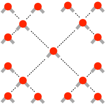
Figure 1: Schematic representation of the fully coordinated water configuration (P₄ population, see text). Dashed lines represent hydrogen bonds

II Methods

II.1 Simulations

Molecular dynamics simulations were run with the program GROMACS gromacs with an integration time-step of 2 fs. The water box consisted of 1024 water molecules in the NPT ensemble with pressure of 1 atm and temperatures ranging from 210 K to 350 K with steps of 10 K. The Berendsen barostat Berendsen1984 , velocity rescale thermostat Bussi2007 and PME Darden1993 were used for pressure coupling, temperature coupling and long-range electrostatics, respectively.

The present analysis was done over 25’000 snapshots obtained from a 100 ps long run after a 10 ns equilibration in the same conditions. The short length of the analyzed trajectory is justified because structural properties are calculated for each water molecule, effectively improving the sampling by three order of magnitudes (there are 1024 water molecules). Repeating the analysis with a longer equilibration time reproduced the same results. TIP5P data was collected up to 230 K, just before the approaching of the glass-transition Brovchenko2005 .

II.2 Density maximum

The position of the maximum density was obtained from 1 ns long simulations after 10 ns of equilibration in the NPT ensemble. The temperature of maximum density was extracted by polynomial fitting around the maximum. Variations from the literature (see Table 1) may be due to size effects and a different treatment of the electrostatics. The location of the TIP3P density maximum was obtained by running further simulations at lower temperatures.

II.3 Energetics and tetrahedral order parameter

The free energy of a configuration $i$ is given by

$$\Delta F_{i}=-k_{B}T\log(P_{i}),$$ (1)

where $k_{B}$ is the Boltzmann factor, $T$ the temperature and $P_{i}$ the population of the selected configuration. The enthalpy is estimated by summing up all pairwise contributions between the water molecules belonging to the same configuration.

The tetrahedral order parameter for a water molecule $i$ is calculated as

$$q_{i}=1-\frac{3}{8}\sum_{j=1}^{3}\sum_{k=j+1}^{4}\big{(}cos\psi_{jik}+\frac{1}{3}\big{)}^{2},$$ (2)

where $j$ and $k$ are any of the four nearest water molecules of $i$ and $\psi_{jik}$ is the angle formed by their oxygensErrington2001 . The averaged value of this order parameter over an ensemble of water molecules is denoted as $Q$.

III Results

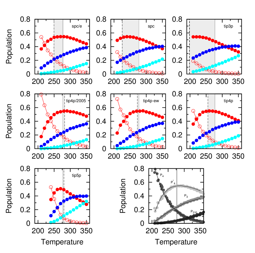
Figure 2: Temperature dependence of water structure populations for seven classical water models. P₄, P${}_{4}^{*}$, P₃, and P₂₁₀ are shown in red empty, filled red, blue, and light blue circles, respectively (see text for details). The gray stretch highlights the temperature difference between the calculated position of the temperature of maximum density (vertical dashed line, see also Table 1) and the experimental value at 277 K (solid line). The bottom right monochrome plot shows the superposition of all models after temperature shifting each data set (TIP4P/2005 data was used as reference). For each temperature, the sum over the 4 groups is equal to one.

III.1 Structure forming capabilities

Water structure forming capabilities were investigated by analyzing the hydrogen-bond network of each water molecule in the simulation box together with its first and second solvation shells. A maximum of four hydrogen-bonds per molecule was considered. A bond is formed when the distance between oxygens and the angle O-H-O is smaller than 3.5 Å and 30 degrees, respectively Luzar1996 . Water structures were grouped into four archetypal configurations of population P${}_{i}^{(*)}$: the fully coordinated first and second solvation shells for a total of 16 hydrogen-bonds (P₄, see Fig. 1 for a schematic representation); the fully coordinated first shell, in which one or more hydrogen bonds between the first and the second shells are missing or loops are formed (P${}_{4}^{*}$); the three coordinated water molecule (P₃) and the rest (P₂₁₀). Within this representation the sum over the four populations is equal to one for each temperature.

In Fig. 2, the temperature dependence of the four microscopic water structures is shown. Among the different water models, the qualitative behavior is strikingly similar. Three main types of temperature scalings were observed: increasing population with decreasing temperature (enthalpically stabilized); increasing population with increasing temperature (entropically stabilized); with a maximum, where a turnover between enthalpic and entropic stabilization takes place at a model dependent temperature. All four water configurations fall into one of these three main classes. The population of the fully ordered structure, P₄, increases with decreasing temperature (Fig. 2, red empty circles). Consequently, this configuration is enthalpically stabilized. This is not the case when defects in the hydrogen bond structure are introduced (P${}_{4}^{*}$, filled red circles). For this configuration the population increases with decreasing temperature until it reaches a maximum in correspondence to a rapid increase of the population of the fully-coordinated configuration. The maximum is located in a temperature range close to the temperature of maximum density of the model under consideration (dashed vertical line). Finally, both P₃ and P₂₁₀ are mainly entropically stabilized, showing larger populations at higher temperatures. Taken together, these results indicate that specific water configurations dominate at each temperature range: full-coordination extending to at least two solvation shells at low temperatures, four-coordinated configurations with no spatial extension at intermediate temperatures and mainly disordered ones at higher temperatures.

Despite these similarities, an important difference among the models is the temperature range at which the relative configurations become dominant. For example, the maximum population of P${}_{4}^{*}$ for the SPC model was observed around $\sim 245$ K (Table 1. This is not the case for TIP4P/2005, where the maximum is located at a 40 K larger temperature. The same behavior was observed comparing the temperatures at which P₄ and P₃ are equal (e.g., around 270 K for TIP4P/2005). These observations suggested that a temperature shift factor ($\Delta T_{s}$) exists among the models. Using TIP4P/2005 as a reference, we found a temperature shift factor for each model ranging from 65 K to 6 K (see Fig. 3 and Table 1). TIP4P/2005 was chosen as reference for its ability to reproduce the density curve Abascal2009 . Applying this shift to the data allowed the superposition of all models onto four master curves, one for each structural configuration, as shown in the monochrome plot at the bottom right of Fig. 2. Our observation is consistent with previously found phase diagram shifts among different water models Sanz2004 ; Vega2005shift as well as in the presence of ions Corradini2011 but in this case we could superimpose all models onto a master curve. Unfortunately, TIP5P had to be excluded from the superposition because all points show an increased curvature with respect to the other models, consistent with the increased curvature of the isobaric density at 1 atm Vega2005 . The structural temperature shift is larger for three-site models (Fig. 3) with a spread of up to 65K for TIP3P. On the other hand, four-site models deviate less. Both SPC-E and TIP4P are characterized by a temperature shift with respect to TIP4P/2005 of around 20K. In general, models providing a better estimation of the position of the density maximum deviate less.

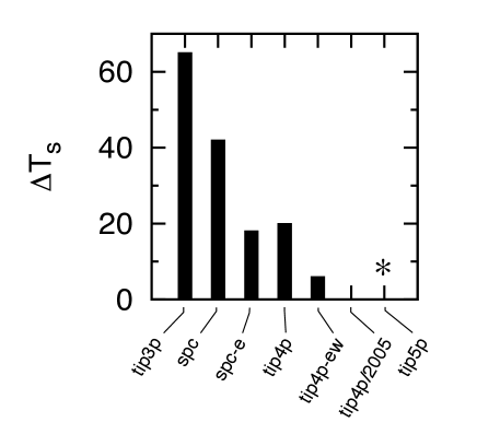
Figure 3: Structural temperature shift $\Delta T_{s}$ with respect to the TIP4P/2005 model. TIP5P was excluded from the superposition analysis (see text for details) .

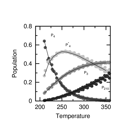
Figure 4: Overlap of the P_i data when a Skinner definition Kumar2007 for the hydrogen bond is used.

In order to check the robustness of the P_i overlap with the hydrogen bond definition, the recent definition of Skinner and collaborators Kumar2007 was applied. Fig. 4 shows that the overlap between the curves is independent from the hydrogen bond definition. Moreover, the temperature shifts calculated in this case are very similar to the ones reported in Table 1. It is interesting to note that this bond definition is very different from the one used in Fig. 2, being based on an empirical fit of the electronic occupancy Kumar2007 .

III.2 Stabilization of the fully coordinated configuration

At all temperatures, water models with smaller shifts provide an improved stabilization of the fully coordinated configuration. (Alternatively, it can be said that these models destabilize poorly hydrogen-bonded configurations). To make this point clearer, the free energy of the fully coordinated configuration at 230K was calculated (Fig. 5a and Methods). At this temperature P₄ is appreciably large for all water models. Comparison with the temperature shifts of Fig. 3 indicates a remarkable correlation where even the small differences between SPC-E and TIP4P are respected (Pearson correlation coefficient of 0.99). The correlation decreases when considering only the enthalpy, as shown in Fig. 5b (correlation of 0.94, see Methods). Interestingly, enthalpy and free energy correlate very well within the same model family. This is particularly clear when looking at the three sites models (i.e., the trend for TIP3P, SPC and SPC/E), suggesting a different entropic contribution between three and four sites models which is systematic.

Finally, the average value of the tetrahedral order parameter $Q$ Errington2001 of the fully coordinated configuration calculated at the same temperature is shown in Fig. 5c. In first approximation, the parameter correlates well with the structural shift although not as good as the free energy (correlation coefficients of 0.98).

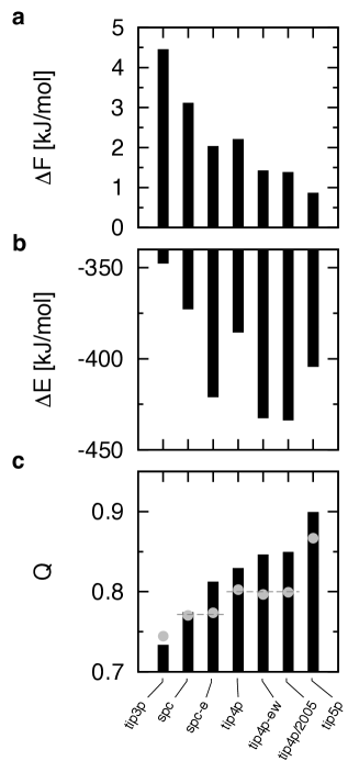
Figure 5: Comparison of water models with respect to the fully coordinated configuration at 230 K. (a) The value of the free energy. (b) Average enthalpy. (c) Average value of the tetrahedral order parameter $Q$. The value of $Q$ for the case P${}_{4}=0.2$ is shown as gray filled circles.

Figure 6: Comparison between the structural temperature shifts ($\Delta T_{s}$) and the position of the density maximum ($\Delta T_{density}$). Four-site models were compared to TIP4P/2005 (filled circles). Three-site models were compared to SPC/E (empty circles). Crosses refer to the case when TIP4P/2005 was used as reference for the three-site models.

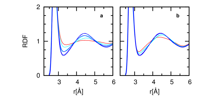
Figure 7: Radial distribution function (RDF) (a) at 270 K; (b) after the application of the temperature shift $\Delta T_{s}$ (see Table I), taking the TIP4P/2005 model at 270 K as reference. TIP3P, SPC and TIP4P families are shown in red, light blue and blue, respectively.

III.3 Comparison with the position of the density maximum

It is worth commenting on the relation between the structural temperature shifts found in this work and the model-dependent temperature of maximum density. As shown in Fig. 6 and Table 1, the relationship between the structural $\Delta T_{s}$ and the density $\Delta T_{density}$ temperature shifts is linear within the three or the four-sites models (filled and empty circles in Fig. 6). However, when comparing all models together using TIP4P/2005 as reference a small systematic deviation is observed (filled circles and crosses in the figure). This is due to the relation that exists between the populations P_i and the density. It is noted that the relative position of the P${}_{4}^{*}$ maximum with respect to the temperature of maximum density (dashed line in Fig. 2, see also Table 1) depends on the model family. For four-sites models the two temperatures are identical, while for three and five-sites models the maximum of P${}_{4}^{*}$ is found at a higher and a lower temperature, respectively. This behavior might be connected with the systematic deviations between free energy and enthalpy for the different water models (Fig. 5a-b).

To better elucidate the connection with the temperature shifts, the radial distribution function (RDF) was calculated. At 270 K the RDF for the various models shows a different structural signature (Fig. 7a). As expected, only the curves for TIP4P/2005 and TIP4P-Ew overlap, being the two models very similar. In Fig. 7b the RDF was recalculated at temperatures shifted according to $\Delta T_{s}$ using as reference TIP4P/2005 at 270 K. The figure shows that all models with the same geometry perfectly overlap (e.g. TIP4P, TIP4P-Ew and TIP4P/2005, blue lines), suggesting that model reparametrizations act as an effective shift in temperature space. On the other hand, changes in the geometry or the number of sites affect the general shape of the radial distribution function and consequently the density.

Similar conclusions can be deduced when calculating the tetrahedral order parameter $Q$ for temperatures at which the fully coordinated structure has the same probability for all models (P${}_{4}=0.2$, gray filled circles in Fig. 5c). $Q$ takes the same value within a given family but it is influenced by the change of the molecular geometry, indicating that the structure corresponding to fully coordinated waters depends on the model family.

IV Conclusions

In conclusion, we found that seven among the most used classical water models are characterized by very similar hydrogen-bond structure-forming capabilities up to a temperature shift. All models but TIP5P perfectly overlap onto a master curve when this shift is applied. This behavior does not depend on the hydrogen-bond definition. Our findings suggest that model reparametrization acts as an effective shift in temperature space. On the other hand, changes in the geometry or the number of sites cannot be fully reconducted to temperature shifts alone as shown by the analysis of the density as well as the radial distribution function. As such, although the hydrogen bond topology is universal when applying a certain temperature shift, this is not the case for the structure, each model family being characterized by its own signature.

We found that the three water models optimized to reproduce the position of the density maximum (i.e., TIP4P-Ew, TIP4P/2005 and TIP5P) systematically improve the stabilization of fully coordinated water configurations with an extension of at least two solvation shells. Based on this observation, we speculate that the improvements of these models for biomolecular simulations Best2010 ; Nerenberg2011 are connected to the higher stabilization of ordered water. This property has important implications for the solvation of biomolecules, changing the balance between solute-solute and solute-solvent interactions.

Development of improved force-fields strongly depends on this balance. Our analysis provides a microscopic and reductionist approach to face this challenge.

Table 1: Temperature of maximum density calculated from our simulations (TMD), as found in the literature (TMD^ref), the structural temperature shift ($\Delta T_{s}$) and the temperature at which P${}^{*}_{4}$ is maximum for the seven water models investigated in this work.

Water model	TMD	TMDref	$\Delta T_{s}$	$T_{max(P4^{*})}$
TIP3P	199	182Vega2005	65	229
SPC	226	228Vega2005	42	247
SPC/E	250	241Rick2004	18	275
TIP4P	256	248Jorgensen1983	20	268
TIP4P/2005	280	278Abascal2005	0	287
TIP4P-Ew	273	274Horn2004	6	281
TIP5P	282	285Lisal2002	n.a.	269

References

- (1) Yaakov Levy and José N. Onuchic. Water mediation in protein folding and molecular recognition. Annu. Rev. Biophys. Biomol. Struct., 35(1):389–415, 2006.
- (2) Garegin A. Papoian, Johan Ulander, and Peter G. Wolynes. Role of water mediated interactions in protein-protein recognition landscapes. J. Am. Chem. Soc., 125(30):9170–9178, 2003.
- (3) Gerhard Hummer. Molecular binding: Under water’s influence. Nature Chem., 2(11):906–907, 2010.
- (4) Mazen Ahmad, Wei Gu, Tihamer Geyer, and Volkhard Helms. Adhesive water networks facilitate binding of protein interfaces. Nat. Commun., 2:261, 2011.
- (5) D. Thirumalai, G. Reddy, and J. E. Straub. Role of water in protein aggregation and amyloid polymorphism. Acc. Chem. Res., 45:83–92, 2011.
- (6) Jose L. F. Abascal, Eduardo Sanz, and Carlos Vega. Triple points and coexistence properties of the dense phases of water calculated using computer simulation. Phys. Chem. Chem. Phys., 11:556–562, 2009.
- (7) J. L. Aragones, L. G. MacDowell, J. I. Siepmann, and C. Vega. Phase diagram of water under an applied electric field. Phys. Rev. Lett., 107:155702, Oct 2011.
- (8) C. Vega and J. L. F. Abascal. Relation between the melting temperature and the temperature of maximum density for the most common models of water. J. Chem. Phys., 123(14):144504, 2005.
- (9) J. L. F. Abascal and C. Vega. A general purpose model for the condensed phases of water: TIP4P/2005. J. Chem. Phys., 123(23):234505, 2005.
- (10) George S. Kell. Density, thermal expansivity, and compressibility of liquid water from to . correlations and tables for atmospheric pressure and saturation reviewed and expressed on 1968 temperature scale. J. Chem. Eng. Data, 20(1):97–105, 1975.
- (11) William L. Jorgensen, Jayaraman Chandrasekhar, Jeffry D. Madura, Roger W. Impey, and Michael L. Klein. Comparison of simple potential functions for simulating liquid water. J. Chem. Phys., 79(2):926–935, 1983.
- (12) H. J. C. Berendsen, J. P. M. Postma, W. F. van Gunsteren, and J. Hermans. Interaction models for water in relation to protein hydration. Intermolecular Forces, 11((Suppl. 1)):331–338, 1981.
- (13) Petra Florová, Petr Sklenovský, Pavel Banáš, and Michal Otyepka. Explicit Water Models Affect the Specific Solvation and Dynamics of Unfolded Peptides While the Conformational Behavior and Flexibility of Folded Peptides Remain Intact. J. Chem. Theory Comput., 6(11):3569–3579, 2010.
- (14) Robert B. Best and Jeetain Mittal. Protein simulations with an optimized water model: cooperative helix formation and temperature-induced unfolded state collapse. J. Phys. Chem. B, 114(46):14916–14923, 2010.
- (15) Paul S. Nerenberg and Teresa Head-Gordon. Optimizing protein-solvent force fields to reproduce intrinsic conformational preferences of model peptides. J. Chem. Theory Comput., 7:1220–1230, 2011.
- (16) H. J. C. Berendsen, J. R. Grigera, and T. P. Straatsma. The missing term in effective pair potentials. J. Phys. Chem., 91(24):6269–6271, 1987.
- (17) William L. Jorgensen and Jeffry D. Madura. Temperature and size dependence for monte carlo simulations of TIP4P water. Mol. Phys., 56(6):1381–1392, 1985.
- (18) Hans W. Horn, William C. Swope, Jed W. Pitera, Jeffry D. Madura, Thomas J. Dick, Greg L. Hura, and Teresa Head-Gordon. Development of an improved four-site water model for biomolecular simulations: TIP4P-Ew. J. Chem. Phys., 120(20):9665–9678, 2004.
- (19) Michael W. Mahoney and William L. Jorgensen. A five-site model for liquid water and the reproduction of the density anomaly by rigid, nonpolarizable potential functions. J. Chem. Phys., 112(20):8910–8922, 2000.
- (20) Francesco Rao, Sean Garrett-Roe, and Peter Hamm. Structural inhomogeneity of water by complex network analysis. J. Phys. Chem. B, 114(47):15598–15604, 2010.
- (21) S. Garrett-Roe, F. Perakis, F. Rao, and P. Hamm. Three-dimensional infrared spectroscopy of isotope-substituted liquid water reveals heterogeneous dynamics. J. Phys. Chem. B, 115(21):6976–6984, 2011.
- (22) David Van Der Spoel, Erik Lindahl, Berk Hess, Gerrit Groenhof, Alan E. Mark, and Herman J. C. Berendsen. GROMACS: Fast, flexible, and free. J. Comput. Chem., 26(16):1701–1718, 2005.
- (23) H. J. C. Berendsen, J. P. M. Postma, W. F. van Gunsteren, A. DiNola, and J. R. Haak. Molecular dynamics with coupling to an external bath. J. Chem. Phys., 81(8):3684–3690, 1984.
- (24) Giovanni Bussi, Davide Donadio, and Michele Parrinello. Canonical sampling through velocity rescaling. J. Chem. Phys., 126(1):014101, 2007.
- (25) Tom Darden, Darrin York, and Lee Pedersen. Particle mesh ewald: An n log(n) method for ewald sums in large systems. J. Chem. Phys., 98(12):10089–10092, 1993.
- (26) Ivan Brovchenko, Alfons Geiger, and Alla Oleinikova. Liquid-liquid phase transitions in supercooled water studied by computer simulations of various water models. J. Chem. Phys., 123(4):044515, 2005.
- (27) J. R. Errington and P. G. Debenedetti. Relationship between structural order and the anomalies of liquid water . Nature, 409(6818):318–321, 2001.
- (28) A. Luzar and D. Chandler. Effect of Environment on Hydrogen Bond Dynamics in Liquid Water. Phys. Rev. Lett., 76:928–931, 1996.
- (29) E. Sanz, C. Vega, J. L. F. Abascal, and L. G. MacDowell. Phase diagram of water from computer simulation. Phys. Rev. Lett., 92:255701, 2004.
- (30) C. Vega, E. Sanz, and J. L. F. Abascal. The melting temperature of the most common models of water. J. Chem. Phys., 122(11):114507, 2005.
- (31) D. Corradini and P. Gallo. Liquid-liquid coexistence in nacl aqueous solutions: a simulation study of concentration effects. J. Phys. Chem. B, 115(48):14161–14166, 2011.
- (32) R. Kumar, J. R. Schmidt, and J. L. Skinner. Hydrogen bonding definitions and dynamics in liquid water. J. Chem. Phys., 126(20):204107, 2007.
- (33) S. W. Rick. A reoptimization of the five-site water potential (tip5p) for use with ewald sums. J. Chem. Phys., 120(13):6085–6093, 2004.
- (34) Martin Lisal, Jiri Kolafa, and Ivo Nezbeda. An examination of the five-site potential (tip5p) for water. J. Chem. Phys., 117(19):8892–8897, 2002.