Robust two-dimensional subrecoil Raman cooling
by adiabatic transfer in a tripod atomic system

Abstract

We demonstrate two-dimensional robust Raman cooling in a four-level tripod system, in which velocity-selective population transfer is achieved by a STIRAP pulse. In contrast to basic 2D Raman cooling with square envelope pulses [Phys. Rev. A 83, 023407 (2011)], the technique presented here allows for a wide variation in the pulse duration and amplitude once the adiabaticity criterion is satisfied. An efficient population transfer together with attaining of a narrow spread of the resonant-velocity group leads to the narrowing of the velocity-distribution spread down to $0.1v_{\mathrm{rec}}$, corresponding to an effective temperature equal to $0.01T_{\mathrm{rec}}$. This robust method opens new possibilities for cooling of neutral atoms.

I Introduction

Control of the atomic degrees of freedom at low temperatures is the starting point for many promising and popular research fields which aim either at understanding and simulating the quantum nature of particle collisions Weiner1999 , photoassociation of atoms into molecules Calsamiglia2001 ; Jones2006 , many-body effects Bloch2008 and phase transitions Dziarmaga2010 , or at applications such as quantum computers Nielsen2000 ; Stenholm2005 and atomic clocks Audoin2001 ; Ye2008 ; Derevianko2011 . Most effects are best observed at ultralow temperatures, which can be nowadays achieved for neutral atoms by a combination of laser cooling and subsequent evaporative cooling Cohen2011 . The latter process requires also trapping of atoms, usually with a very tight confinement, which then precludes efficient use of the method e.g. for collimation of slow atomic beams Johnson1998 ; Theuer1999 ; Partlow2004 or in only partially trapped systems such as one-dimensional optical lattices Lewenstein2012 . The latter situation is utilized e.g. in optical atomic clocks Ye2008 ; Derevianko2011 . Although tight confinement and the subsequent discrete motional state structure for atoms offers many methods for further cooling in a manner similar to the cooling of trapped ions Morigi1997 ; Schmidt-Kaler2001 ; Leibfried2003 and open possibilities for other interesting studies as quantum computing Cirac1995 ; Haffner2008 and entanglement Roghani2008 ; Roghani2011 ; Roghani2012 , alternative approaches are needed in order to apply cooling at a more general setting such as free space. This is the motivation for developing further purely light-based methods for reaching similar temperatures as with evaporative cooling, as discussed also in our previous work on the topic Ivanov2011 ; Ivanov2012 .

In the past, powerful cooling techniques have been designed to achieve subrecoil temperatures of free atoms. The “dark state” cooling Aspect1988 is very efficient but also limited to rather collisionless situations (low densities). Raman cooling, on the other hand, is not so density-limited, and deep subrecoil cooling in 1D has been demonstrated Kasevich1992 and extended to 2D and 3D cooling Davidson1994 ; Boyer2004 as well. The lowest temperature in 2D, achieved for Cs atoms at NIST, Gaithersburg, is 0.15$T_{\mathrm{rec}}$ Boyer2004 , where $T_{\mathrm{rec}}$ is the atomic recoil temperature. The suppression of further cooling is associated with the required cumbersome setup of four Raman beam pairs as well as limitations of the assumed $\Lambda$-type atomic state system. Our recent suggestion of cooling in a tripod atomic level system not only reduces the number of Raman beams by a factor of two, but also allows one, in principle, to reach temperatures as low as $0.01T_{\mathrm{rec}}$. However, more cooling cycles are required in 2D Raman cooling as compared with 1D, which imposes strict demands on the velocity precision of the Raman transfer Ivanov2011 .

To overcome such a limitation, one can employ the robust transfer process provided by STIRAP, as recently suggested by us for 1D Raman cooling Ivanov2012 . However, the process of transferring atoms collected in the atomic “dark state” is not a trivial extension of the 1D situation, and thereby the 2D case is of special consideration. So far, STIRAP in a tripod system by resonant laser beams has been experimentally explored only for atomic beams Theuer1999 , although far-off resonant lasers in general are used for Raman cooling. This paper demonstrates theoretically 2D Raman cooling by STIRAP going down to $0.01T_{\mathrm{rec}}$, which nevertheless allows a wide variation in both the pulse envelope and duration if only the adiabaticity criterion is satisfied. The pulse duration needed for transfer exceeds the pulse durations for normal Raman processes, so the advantage of robustness is attained only if the cooling time is not a critical factor. This slowness related to adiabaticity would restrict the application of the method in atomic beam collimation to very slow beams. Another limitation arises from the specific need for a tripod structure, which is not present e.g. at the main transitions for the alkaline-earth atoms Machholm2001 ; Machholm2002 that are currently the strongest candidate for optical atomic clocks Ye2008 ; Derevianko2011 .

The organization of this paper is as follows. The necessary atomic tripod energy state diagram and the corresponding 2D laser beam configuration are presented and discussed in Sec. II. In Sec. III we show that, as expected, large detuning from the excited atomic state suppresses spontaneous decay, and the resonant-velocity group of STIRAP under this condition is discussed in Sec. IV. An efficient transfer of the atoms from the original ground state, even in the case of such a large detuning, leads to efficient 2D cooling, for which the parameters are given in Sec. V. The cooling itself is investigated in Sec. VI, and our research is concluded by the summary and discussion given in Sec. VII.

II Tripod system and laser configuration

Consider a tripod system under conditions following closely metastable Ne in Ref. Theuer1999 . Pump laser couples state ($2p^{5}3s$) ${}^{3}P_{0}$ to an intermediate state ($2p^{5}3p$) ${}^{3}P_{1}$ ($M=0$) which in turn is coupled to magnetic substates $M=\pm 1$ of ($2p^{5}3s$) ${}^{3}P_{2}$ by two Stokes lasers. The pump laser is a $\pi$-polarized running wave propagating along axis $Oy$, and the Stokes lasers are contra-propagating $\sigma$-polarized running waves arranged along the $Oz$ axis (see Fig. 1(a)). Note that the metastable Ne system is used only as an example. The classical electric field of all three laser beams is written as

$$\mathbf{E}(\mathbf{r},t) =\frac{1}{2}\mathbf{E}_{P}e^{i\mathbf{k}_{P}\mathbf{r}-i\omega_{P}t}+\frac{1}{2}\mathbf{E}_{S}^{+}e^{i\mathbf{k}_{S}\mathbf{r}-i\omega_{S}^{+}t}$$

$$+\frac{1}{2}\mathbf{E}_{S}^{-}e^{-i\mathbf{k}_{S}\mathbf{r}-i\omega_{S}^{-}t}+\text{c.c.}$$ (1)

The first term corresponds to pump laser with frequency $\omega_{P}$ and wave vector $\mathbf{k}_{P}=k_{P}\mathbf{e}_{y}$; the two other terms relatively correspond to $\sigma^{+}$- and $\sigma^{-}$-polarized Stokes lasers with frequencies $\omega_{S}^{+}$, $\omega_{S}^{-}$ and wave vectors $\mathbf{k}_{S}$, $-\mathbf{k}_{S}$, where $\mathbf{k}_{S}=k_{S}\mathbf{e}_{z}$.

(a)

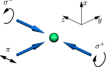
(b)

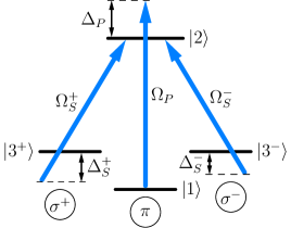
(c)

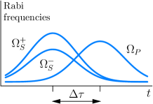
Figure 1: (Color online) (a) The 2D laser configuration consists of three running waves, two circularly-polarized waves arranged along the $Oz$ axis and a $\pi$-polarized wave propagating in the $Oy$ direction. (b) The energy-level diagram of the tripod system coupled by laser beams. (c) Both Stokes pulses $\Omega_{S}^{+}(t)$ and $\Omega_{S}^{-}(t)$ forms a counterintuitive sequence with the pump pulse $\Omega_{P}(t)$ in order to carry out atomic population from state $|1\rangle$ to $|3^{+}\rangle$ and $|3^{-}\rangle$, respectively.

Figure 1(b) illustrates the atomic states coupled by the laser configuration, with labelling

$$\begin{aligned} &|1\rangle=|(2p^{5}3s)\;^{3}P_{0},M=0\rangle,\\ &|2\rangle=|(2p^{5}3p)\;^{3}P_{1},M=0\rangle,\\ &|3^{+}\rangle=|(2p^{5}3s)\;^{3}P_{2},M=-1\rangle,\\ &|3^{-}\rangle=|(2p^{5}3s)\;^{3}P_{2},M=1\rangle.\end{aligned}$$ (2)

Taking into account shifts in the centre-of-mass momentum, we consider an atom of momentum $\mathbf{p}$ originally prepared in state $|1,\mathbf{p}\rangle$. Then laser-atom coupling strengths are given by

$$\begin{aligned} &\hat{V}|1,\mathbf{p}\rangle=\frac{\hbar}{2}\Omega_{P}(t)e^{-i\omega_{P}t}|2,\mathbf{p}+\hbar\mathbf{k}_{P}\rangle,\\ &\hat{V}|3^{\pm},\mathbf{p}+\hbar\mathbf{k}_{P}\mp\hbar\mathbf{k}_{S}\rangle=\frac{\hbar}{2}\Omega_{S}^{\pm}(t)e^{-i\omega_{S}^{\pm}t}|2,\mathbf{p}+\hbar\mathbf{k}_{P}\rangle,\end{aligned}$$ (3)

where $\hat{V}$ is the coupling operator in rotating wave approximation (RWA); the Rabi frequencies

$$\Omega_{P}(t)=-\frac{\mathbf{d}_{21}\mathbf{E}_{P}}{\hbar},\quad\Omega_{S}^{\pm}(t)=-\frac{\mathbf{d}_{23}^{\pm}\mathbf{E}_{S}^{\pm}}{\hbar},$$ (4)

are assumed to be real-valued; $\mathbf{d}_{21}$, $\mathbf{d}_{23}^{\pm}$ are the matrix elements of the dipole moment operator. Rabi frequencies (4) evolve in time together with the electric field components $\mathbf{E}_{P}$, $\mathbf{E}_{S}^{+}$ and $\mathbf{E}_{S}^{-}$, and have Gaussian envelopes arranged in a counterintuitive sequence as shown in Fig. 1(c):

$$\begin{aligned} &\Omega_{P}(t)=\Omega_{P0}e^{-(t-t_{P})^{2}/2T_{P}^{2}},\\ &\Omega_{S}^{\pm}(t)=\Omega_{S0}^{\pm}e^{-(t-t_{S})^{2}/2T_{S}^{2}},\end{aligned}$$ (5)

where $t_{S}<t_{P}$; here $2T_{P}$, $2T_{S}$ are the corresponding pulse widths.

In addition to the atom-field coupling $\hat{V}$, the total Hamiltonian for the atom-field system

$$\hat{H}=\hat{H}_{0}+\frac{\hat{\mathbf{P}}^{2}}{2M}+\hat{V}$$

includes the kinetic term $\hat{\mathbf{P}}^{2}/(2M)$, and the energy $\hat{H}_{0}$ of a non-moving atom with the internal state energies $E_{1}$, $E_{2}$, $E_{3}^{+}$ and $E_{3}^{-}$. As long as spontaneous emission is not taken into account, the atomic states in the tripod system form a closed family of momentum $\mathbf{p}$:

$$\mathcal{F}(\mathbf{p})=\{|1,\mathbf{p}\rangle,|2,\mathbf{p}+\hbar\mathbf{k}_{P}\rangle,\\ |3^{+},\mathbf{p}+\hbar\mathbf{k}_{P}-\hbar\mathbf{k}_{S}\rangle,|3^{-},\mathbf{p}+\hbar\mathbf{k}_{P}+\hbar\mathbf{k}_{S}\rangle\}.$$ (6)

As a result, in the basis of four bare states,

$$\begin{aligned} |a_{1}\rangle=&\exp\biggl{[}-i\biggl{(}\frac{E_{1}}{\hbar}+\frac{\mathbf{p}^{2}}{2M\hbar}\biggr{)}t\biggr{]}|1,\mathbf{p}\rangle,\\ |a_{2}\rangle=&\exp\biggl{[}-i\biggl{(}\frac{E_{2}}{\hbar}+\frac{\mathbf{p}^{2}}{2M\hbar}+\Delta_{P}\biggr{)}t\biggr{]}|2,\mathbf{p}+\hbar\mathbf{k}_{P}\rangle,\\ |a_{3}^{\pm}\rangle=&\exp\biggl{[}-i\biggl{(}\frac{E_{3}^{\pm}}{\hbar}+\frac{\mathbf{p}^{2}}{2M\hbar}+\Delta_{P}-\Delta_{S}^{\pm}\biggr{)}t\biggr{]}\\ &\times|3^{\pm},\mathbf{p}+\hbar\mathbf{k}_{P}\mp\hbar\mathbf{k}_{S}\rangle,\end{aligned}$$ (7)

the dynamics of the atom is described by the atomic Hamiltonian

$$H=\frac{\hbar}{2}\begin{pmatrix}0&\Omega_{P}(t)&0&0\\ \Omega_{P}(t)&-2\tilde{\Delta}_{P}&\Omega_{S}^{+}(t)&\Omega_{S}^{-}(t)\\ 0&\Omega_{S}^{+}(t)&2\delta_{S}^{+}&0\\ 0&\Omega_{S}^{-}(t)&0&2\delta_{S}^{-}\end{pmatrix},$$ (8)

with the following detunings:

$$\begin{aligned} \tilde{\Delta}_{P}&=\Delta_{P}-\frac{k_{P}p_{y}}{M}-\omega^{R}_{P},\\ \delta_{S}^{\pm}&=\Delta_{S}^{\pm}-\Delta_{P}+\frac{k_{P}p_{y}\mp k_{S}p_{z}}{M}+\omega^{R}_{P}+\omega^{R}_{S}.\end{aligned}$$ (9)

Here, $p_{y}$, $p_{z}$ are projections of momentum $\mathbf{p}$ on axes $Oy$ and $Oz$, respectively; $\Delta_{P}=\omega_{P}-\omega_{21}$, $\Delta_{S}^{\pm}=\omega_{S}^{\pm}-\omega_{23}^{\pm}$ are the laser detunings; $\omega^{R}_{P}=\hbar k_{P}^{2}/(2M)$, $\omega^{R}_{S}=\hbar k_{S}^{2}/(2M)$ are the one-photon recoil frequencies.

III Suppression of upper-state decay

The first step of a cooling cycle demands that the contribution of upper-state decay is as low as possible, because the decay broadens the velocity spread of population transfer and thus suppresses the control required by subrecoil cooling. To avoid the undesirable spontaneous decay, sufficiently large upper-state detunings $\Delta_{P}$ are commonly utilized. Here such approach means that we need to satisfy the conditions

$$|\Delta_{P}|\gg\frac{k_{P}p_{y}}{M},\frac{k_{S}p_{z}}{M},\omega^{R}_{P},\omega^{R}_{S}.$$ (10)

Then the upper state is adiabatically eliminated from the Hamiltonian (8) and we can write

$$\langle a_{2}|\Psi\rangle\approx\frac{\Omega_{P}(t)}{2\Delta_{P}}\langle a_{1}|\Psi\rangle+\frac{\Omega_{S}^{+}(t)}{2\Delta_{P}}\langle a_{3}^{+}|\Psi\rangle+\frac{\Omega_{S}^{-}(t)}{2\Delta_{P}}\langle a_{3}^{-}|\Psi\rangle,$$ (11)

where $|\Psi\rangle$ is the wave function of an atom. In turn, Eq. (11) relies on the adiabaticity constraint

$$|\langle a_{2}|\frac{d}{dt}|\Psi\rangle|\ll|\Delta_{P}||\langle a_{2}|\Psi\rangle|,$$ (12)

which gives the necessary conditions for the validity of the upper-state elimination, namely

$$|\Delta_{P}|\gg\Omega_{P0},\Omega_{S0}^{\pm},|\delta_{S}^{\pm}|,T^{-1}.$$ (13)

The latter term shows that the envelopes of the laser pulses should evolve in time with a rate that is much smaller than the upper-state detuning in frequency units, whereas the other terms in the right-hand side respond to the splitting of the atomic levels. Then, the reduced Hamiltonian in the basis of states $\{|1\rangle,|3^{+}\rangle,|3^{-}\rangle\}$ is written as

$$\tilde{H}=\frac{\hbar}{2}\begin{pmatrix}\dfrac{\Omega_{P}(t)^{2}}{2\Delta_{P}}&\dfrac{\Omega_{P}(t)\Omega_{S}^{+}(t)}{2\Delta_{P}}&\dfrac{\Omega_{P}(t)\Omega_{S}^{-}(t)}{2\Delta_{P}}\\ \dfrac{\Omega_{P}(t)\Omega_{S}^{+}(t)}{2\Delta_{P}}&2\delta_{S}^{+}+\dfrac{\Omega_{S}^{+}(t)^{2}}{2\Delta_{P}}&\dfrac{\Omega_{S}^{+}(t)\Omega_{S}^{-}(t)}{2\Delta_{P}}\\ \dfrac{\Omega_{P}(t)\Omega_{S}^{-}(t)}{2\Delta_{P}}&\dfrac{\Omega_{S}^{+}(t)\Omega_{S}^{-}(t)}{2\Delta_{P}}&2\delta_{S}^{-}+\dfrac{\Omega_{S}^{-}(t)^{2}}{2\Delta_{P}}\end{pmatrix}.$$ (14)

The contribution of spontaneous decay is estimated as the loss of population from the upper state of natural width $\Gamma$ during STIRAP process. With help of the density operator $\hat{\sigma}$, whose matrix elements are

$$\sigma_{ij}(\mathbf{p})=\langle a_{i}|\hat{\sigma}|a_{j}\rangle,\quad i,j=1,2,3^{+},3^{-},$$ (15)

the population loss is given by

$$\frac{d}{dt}\sigma_{\mathrm{sp}}(\mathbf{p})=\Gamma\sigma_{22}(\mathbf{p}),\quad\sigma_{\mathrm{sp}}(\mathbf{p})=\Gamma\int_{0}^{\Delta\tau}\sigma_{22}(\mathbf{p})dt,$$ (16)

occurring during time interval $\Delta\tau$ while the STIRAP pulses overlap. Because the adiabatic process takes a long time, the overall population loss $\sigma_{\mathrm{sp}}(\mathbf{p})$ can not be neglected at this point. To estimate $\sigma_{\mathrm{sp}}(\mathbf{p})$, notice that the condition in Eq. (11) for upper-state elimination leads to the following inequality:

$$\sigma_{22}(\mathbf{p})\lesssim 3\left(\frac{\Omega_{P}(t)^{2}}{4\Delta_{P}^{2}}\sigma_{11}(\mathbf{p})+\frac{\Omega_{S}^{+}(t)^{2}}{4\Delta_{P}^{2}}\sigma_{33}^{++}(\mathbf{p})\right.\\ \left.+\frac{\Omega_{S}^{-}(t)^{2}}{4\Delta_{P}^{2}}\sigma_{33}^{--}(\mathbf{p})\right)\leq 3\frac{\Omega_{P}(t)^{2}+\Omega_{S}^{+}(t)^{2}+\Omega_{S}^{-}(t)^{2}}{4\Delta_{P}^{2}}.$$ (17)

The effect of the spontaneous decay is now estimated by

$$\sigma_{\mathrm{sp}}(\mathbf{p})\leq 3\Gamma\frac{\Omega_{P}(t)^{2}+\Omega_{S}^{+}(t)^{2}+\Omega_{S}^{-}(t)^{2}}{4\Delta_{P}^{2}}\Delta\tau,$$ (18)

and it can be neglected when $\sigma_{\mathrm{sp}}(\mathbf{p})\ll 1$. So, if the constraint

$$\frac{|\Delta_{P}|}{\Gamma}\gg\frac{\Omega_{P}(t)^{2}+\Omega_{S}^{+}(t)^{2}+\Omega_{S}^{-}(t)^{2}}{|\Delta_{P}|}\Delta\tau$$ (19)

is satisfied, then the upper-state decay can be neglected from consideration.

IV Elementary cooling cycle

In the first cooling step, STIRAP only accomplishes a transfer of atoms through the dark state formed by the ground states of the tripod system, thereby determining the velocity selectivity of the transfer. As a combination of the original ground state $|1\rangle$ with either the $|3^{+}\rangle$ or $|3^{-}\rangle$ state, the dark state occurs under the condition of the two-photon resonance between selected ground states. The associated resonant velocities follow from the Hamiltonian in Eq. (8) by setting

$$\delta_{S}^{+}=0\quad\mbox{or}\quad\delta_{S}^{-}=0.$$ (20)

The former condition corresponds to population transfer by Raman transition $|1\rangle\leftrightarrow|3^{+}\rangle$, whereas the latter corresponds to the $|1\rangle\leftrightarrow|3^{-}\rangle$ transition.

Figures 2(a) and (b) illustrate how the atoms are transferred into the $|3^{+}\rangle$ and $|3^{-}\rangle$ states depending on their velocity, and the corresponding hole burning for atoms in state $|1\rangle$ is shown in Fig. 2(c). The use of both transitions for transferring the dark-state atoms from the ground state $|1\rangle$ is an obvious advantage of the tripod system, because atoms can be simultaneously cooled in both dimensions. Form of the burned cross-like hole is defined by the laser configuration. The only variable part is the position of the cross-like pattern, whose center is given by

$$\delta_{S}^{+}=\delta_{S}^{-}=0,$$ (21)

and can be shifted by changing detunings $\Delta_{P}$, $\Delta_{S}^{\pm}$.

(a)

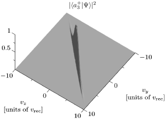
(b)

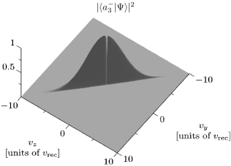
(c)

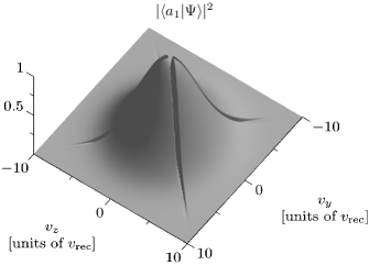
Figure 2: (a) and (b): Parts of the initial velocity distribution transferred by the STIRAP process into the states $|3^{+}\rangle$ and $|3^{-}\rangle$, respectively; (c) The hole burning arising in state $|1\rangle$ due to these transfers. The scaling is given by the recoil velocity $v_{\mathrm{rec}}=\hbar k_{P}/M=\hbar k_{S}/M$ and we also set frequency $\omega^{R}=\omega^{R}_{P}=\omega^{R}_{S}$. The maximal magnitudes $\Omega_{P0}^{2}/|\Delta_{P}|$, $(\Omega_{S0}^{\pm})^{2}/|\Delta_{P}|$ of the two-photon Rabi frequencies are equal to $2\omega^{R}$, and $\Delta_{P}-\Delta_{S}^{\pm}=\omega^{R}$. The STIRAP-pulse duration $T_{\mathrm{pulse}}$ is $96(\omega^{R})^{-1}$.

In order to return atoms from states $|3^{+}\rangle$ and $|3^{-}\rangle$ to the state $|1\rangle$, a fast optical pumping process is needed after the STIRAP pulse. The $\pi$-polarized laser is switched off, and only circularly polarized beams are left, being now tuned into resonance. An atom of momentum $\mathbf{p}$ is excited from either ground state $|3^{+}\rangle$ or $|3^{-}\rangle$ to the upper state and therefore it gains a momentum kick along the $Oz$ direction. Although the momentum kick equals $\hbar\omega_{23}/c$, one can consider that $\omega_{23}/c\approx k_{S}$, and hence the atomic momentum becomes $\mathbf{p}^{\prime}=\mathbf{p}\pm\hbar\mathbf{k}_{S}$. Then the atom decays into the $|1\rangle$ state emitting a spontaneous photon of momentum $\Delta\mathbf{p}$, where $|\Delta\mathbf{p}|=\hbar\omega_{21}/c\approx\hbar k_{P}$. Due to momentum conservation, the atomic momentum changes by $-\Delta\mathbf{p}$, and the population in state $|1\rangle$ takes the form

$$\langle 1,\mathbf{p}|\hat{\sigma}^{\prime}|1,\mathbf{p}\rangle=\langle 1,\mathbf{p}|\hat{\sigma}|1,\mathbf{p}\rangle\\ +\langle 3^{+},\mathbf{p}-\hbar\mathbf{k}_{S}+\Delta\mathbf{p}^{\prime}|\hat{\sigma}|3^{+},\mathbf{p}-\hbar\mathbf{k}_{S}+\Delta\mathbf{p}^{\prime}\rangle\\ +\langle 3^{-},\mathbf{p}+\hbar\mathbf{k}_{S}+\Delta\mathbf{p}^{\prime\prime}|\hat{\sigma}|3^{-},\mathbf{p}+\hbar\mathbf{k}_{S}+\Delta\mathbf{p}^{\prime\prime}\rangle.$$ (22)

In turn, the populations can be expressed in terms of the density matrix elements $\sigma_{ij}(\mathbf{p})$ (15) associated with the momentum family $\mathcal{F}(\mathbf{p})$ (6). Taking into account that states $|a_{j}\rangle$ ($j=1,2,3^{+},3^{-}$) are contained in the same family $\mathcal{F}(\mathbf{p})$, this leads to the expression

$$\sigma^{\prime}_{11}(\mathbf{p})=\sigma_{11}(\mathbf{p})+\sigma_{33}^{++}(\mathbf{p}-\hbar\mathbf{k}_{P}+\Delta\mathbf{p}^{\prime})\\ +\sigma_{33}^{--}(\mathbf{p}-\hbar\mathbf{k}_{P}+\Delta\mathbf{p}^{\prime\prime}),$$ (23)

where momentum shifts are given in relation to $\mathcal{F}(\mathbf{p})$.

In contrast to the first cooling step where an atom is contained in the same family $\mathcal{F}(\mathbf{p})$ during the STIRAP, the optical pumping process mixes the different families $\mathcal{F}(\mathbf{p})$ as shown in Eq. (23). One can see by averaging Eq. (23) over all possible directions of spontaneous decay that an elementary cooling cycle generally pushes the velocity distribution along the $Oy$ axis. If the hole burning center $\mathbf{v}^{0}=\mathbf{p}^{0}/M$ of atoms transferred from state $|1\rangle$ (see Fig. 2(c)) is adjusted to $v_{y}^{0}<0$, then atoms at the left-hand wing on axis $Oy$ are pushed closer to the zero velocity, which leads to the cooling of the atomic ensemble. In addition, a laser configuration with a $\pi$-polarized beam in the opposite direction of propagation and adjustment to $v_{y}^{0}>0$ cools atoms also in the right-side wing of axis $Oy$. When these laser configurations alternate, a cooling of whole the ensemble becomes feasible.

V Resonant group of STIRAP

The efficiency that accompanies the first step of cooling cycle relies on both a narrow velocity range and the entire transfer of resonant-group atoms. In fact, such entire adiabatic transfer occurs if each laser pulse is tuned into resonance with the corresponding atomic transition. Such an approach is efficiently applied in Ref. Korsunsky1996 with the aim of VSCPT cooling. On the other hand, an efficient transfer of dark-state atoms takes place even in the case of large detuning $\Delta_{P}$, as was successfully demonstrated for 1D subrecoil Raman cooling by STIRAP Ivanov2012 .

For velocity-selective STIRAP, a transfer of dark-state atoms from the original state $|1\rangle$ evolves with the efficiency sensitive to the velocity of the dark state. The crossing center defined by Eq. (21) is depleted to a greater extent, because its velocity $\mathbf{v}^{0}$ is attainable for both the $|1\rangle\leftrightarrow|3^{+}\rangle$ and the $|1\rangle\leftrightarrow|3^{-}\rangle$ Raman transitions. For the same reason the velocity spread of the resonant group is widest at the velocity $\mathbf{v}^{0}$. Next we consider the adiabaticity criterion for the population transfer from state $|1\rangle$ at the hole burning center, i.e., for conditions given in Eq. (21).

Instead of assuming the conditions in Eq. (21) directly, we first take the more general case of $\delta_{S}^{+}=\delta_{S}^{-}$ which corresponds to an arbitrary velocity projection $v_{y}$ and

$$v_{z}=\frac{\Delta_{S}^{+}-\Delta_{S}^{-}}{2k_{S}}.$$ (24)

Further, we only consider the case of $\Delta_{S}^{+}=\Delta_{S}^{-}=\Delta_{S}$ when $v_{z}=0$. Such an approach gives us a condition when the zero-velocity atoms do not leave the $|1\rangle$ state and are efficiently accumulated there.

To simplify the equations of motion, we get from the Hamiltonian in Eq. (14) the relationship

$$i\frac{d}{dt}\left(\Omega_{S}^{-}(t)\langle a_{3}^{+}|\Psi\rangle-\Omega_{S}^{+}(t)\langle a_{3}^{-}|\Psi\rangle\right)\\ =(\delta_{S}^{+}+i\Theta(t))\left(\Omega_{S}^{-}(t)\langle a_{3}^{+}|\Psi\rangle-\Omega_{S}^{+}(t)\langle a_{3}^{-}|\Psi\rangle\right),$$ (25)

which only requires that both Stokes pulses, $\Omega_{S}^{+}(t)$ and $\Omega_{S}^{-}(t)$, evolve in time simultaneously:

$$\frac{\dot{\Omega}_{S}^{+}(t)}{\Omega_{S}^{+}(t)}=\frac{\dot{\Omega}_{S}^{-}(t)}{\Omega_{S}^{-}(t)}=\Theta(t).$$ (26)

Before the STIRAP pulse starts, the atoms are contained in state $|1\rangle$. Hence $\langle a_{3}^{+}|\Psi\rangle^{0},\langle a_{3}^{-}|\Psi\rangle^{0}=0$, and one obtains from Eq. (25) that

$$\Omega_{S}^{-}(t)\langle a_{3}^{+}|\Psi\rangle=\Omega_{S}^{+}(t)\langle a_{3}^{-}|\Psi\rangle.$$ (27)

We consider the following coupled (C) and non-coupled (NC) states of the coupling operator in Eq. (3):

$$|\mathrm{C}\rangle=\frac{\Omega_{S}^{+}(t)}{\Omega_{S}(t)}|a_{3}^{+}\rangle+\frac{\Omega_{S}^{-}(t)}{\Omega_{S}(t)}|a_{3}^{-}\rangle,$$ (28)

$$|\mathrm{NC}\rangle=\frac{\Omega_{S}^{-}(t)}{\Omega_{S}(t)}|a_{3}^{+}\rangle-\frac{\Omega_{S}^{+}(t)}{\Omega_{S}(t)}|a_{3}^{-}\rangle,$$ (29)

where $\Omega_{S}(t)^{2}=\Omega_{S}^{+}(t)^{2}+\Omega_{S}^{-}(t)^{2}$. It follows from Eq. (27) that $\langle\mathrm{NC}|\Psi\rangle=0$, which in turn leads to relationships

$$\langle a_{3}^{+}|\Psi\rangle=\frac{\Omega_{S}^{+}(t)}{\Omega_{S}(t)}\langle\mathrm{C}|\Psi\rangle,\quad\langle a_{3}^{-}|\Psi\rangle=\frac{\Omega_{S}^{-}(t)}{\Omega_{S}(t)}\langle\mathrm{C}|\Psi\rangle.$$ (30)

Equation (26) shows that $\Omega_{S}^{\pm}(t)/\Omega_{S}(t)$ are constant during the STIRAP process. Hence the Hamiltonian in Eq. (14) in the basis of states $\{|a_{1}\rangle,|\mathrm{C}\rangle\}$ takes the form

$$\hat{H}_{\mathrm{eff}}=\frac{\hbar}{2}\begin{pmatrix}-2\delta_{0}(t)&\Omega_{\mathrm{eff}}(t)\\ \Omega_{\mathrm{eff}}(t)&2(\delta_{\mathrm{eff}}(t)-\delta_{0}(t))\end{pmatrix}.$$ (31)

The effective detunings and the Rabi frequency are

$$\delta_{0}(t)=-\frac{\Omega_{P}(t)^{2}}{4\Delta_{P}},\quad\Omega_{\mathrm{eff}}(t)=\frac{\Omega_{P}(t)\Omega_{S}(t)}{2\Delta_{P}},$$

$$\delta_{\mathrm{eff}}(t)=\Delta\delta+\frac{\Omega_{S}(t)^{2}-\Omega_{P}^{2}(t)}{4\Delta_{P}},$$ (32)

where detuning $\Delta\delta$ determines the offset from the resonance velocity:

$$\Delta\delta=\Delta_{S}-\Delta_{P}+\frac{k_{P}p_{y}}{M}+\omega^{R}_{P}+\omega^{R}_{S}=k_{P}(v_{y}-v_{y}^{0}).$$ (33)

The Hamiltonian in Eq. (31) describes an effective two-level system considered in Ref. Ivanov2012 . Almost the entire transfer of the resonant-velocity atoms occurs once the following adiabaticity criterion is fulfilled Ivanov2012 :

$$\frac{\Omega_{P}(t)^{2}+\Omega_{S}(t)^{2}}{|\Delta_{P}|}\Delta\tau\gg 1.$$ (34)

The adiabaticity criterion in combination with Eq. (19) gives the conditions

$$\frac{|\Delta_{P}|}{\Gamma}\gg\frac{\Omega_{P}(t)^{2}+\Omega_{S}^{+}(t)^{2}+\Omega_{S}^{-}(t)^{2}}{|\Delta_{P}|}\Delta\tau\gg 1.$$ (35)

This constraint gives the value of $\Delta\tau$, which is needed for achieving an entire transfer of the resonant-group atoms. Unlike with the normal Raman processes using square or Blackman envelopes for pulses, the requirement of having exactly a $\pi$-pulse is not present here. However, the appropriate STIRAP pulses should vary slow enough, which makes the pulse durations larger than those of $\pi$-pulses in normal Raman process. Hence, the STIRAP transfer is suitable in cases where the cooling time is not in any critical role, giving in exchange robustness in setting the actual pulse durations.

The resonant-velocity group can be evaluated in terms of $\Delta\delta$ (Eq. (33)). Taking into account that $\Delta\delta=k_{P}(v_{y}-v_{y}^{0})$ differs from the $\Delta\delta=2k(v-v_{0})$ obtained for the 1D case Ivanov2012 , the velocity spread of the resonant group through $v_{z}=0$ is given by Ivanov2012

$$\begin{aligned} -\frac{(\Omega_{S0}^{+})^{2}+(\Omega_{S0}^{-})^{2}}{2k_{P}|\Delta_{P}|}<v_{y}-v_{y}^{0}<\frac{\Omega_{P0}^{2}}{2k_{P}|\Delta_{P}|}\quad\mbox{if $\Delta_{P}>0$},\\ -\frac{\Omega_{P0}^{2}}{2k_{P}|\Delta_{P}|}<v_{y}-v_{y}^{0}<\frac{(\Omega_{S0}^{+})^{2}+(\Omega_{S0}^{-})^{2}}{2k_{P}|\Delta_{P}|}\quad\mbox{if $\Delta_{P}<0$}.\end{aligned}$$ (36)

One can see that the velocity spread defined by the two-photon Rabi frequencies can get as narrow as needed for deep subrecoil cooling. On the other hand, large Rabi frequencies broaden the velocity profile of the transfer. As a result, an appropriate tuning of the pulse intensities allows one to cool the atomic ensemble substantially below the recoil limit.

VI Full cooling process

A single cooling cycle consists of two steps, namely the population transfer by STIRAP pulse and the subsequent optical pumping which returns the atoms back to the original internal state due to spontaneous decay. We assume that $k_{P}=k_{S}$ and hence $\omega_{P}^{R}=\omega_{S}^{R}=\omega^{R}$. The initial velocity distribution of the atomic ensemble has the spread of $3v_{\mathrm{rec}}$, where $v_{\mathrm{rec}}$ is the common recoil velocity of all STIRAP lasers. The lasers are detuned from the upper state by $\Delta_{P}>0$, and the Rabi frequencies are given by

$$\Omega_{P0}^{2}=(\Omega_{S0}^{+})^{2}=(\Omega_{S0}^{-})^{2}=2k_{P}|v_{y}^{0}||\Delta_{P}|,$$ (37)

suppressing the transfer of zero-velocity atoms. The laser configuration shown in Fig. 1(a) has the resonant velocity of $v_{y}^{0}<0$, whereas the case of the alternated $\pi$-polarized beam corresponds to $v_{y}^{0}>0$. After each sequence of five cooling cycles with

$$|v_{y}^{0}|=2^{k-1}v_{\mathrm{rec}},\quad k=0,\ldots,4,$$ (38)

the direction of $\pi$-polarized laser is alternated. The broad velocity profiles in the set defined in Eq. (38) involve all velocity-distributed atoms in the cooling process, whereas those in a narrow velocity group lead to the actual deep cooling below the recoil limit.

(a)

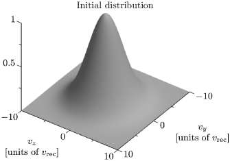
(b)

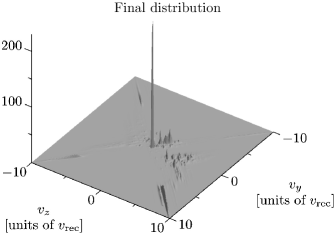
Figure 3: The velocity distribution of an atomic ensemble before (a) and after (b) the 2D cooling is applied. The velocity spread of (a) $3v_{\mathrm{rec}}$ has been reduced to (b) $0.1v_{\mathrm{rec}}$ after realizing 500 single cooling cycles, corresponding to the effective temperature going down to $0.01T_{\text{rec}}$. The height of the central peak has increased to about 230 times that of the initial distribution.

The pump and the Stokes pulses have the same pulse shape with the pulse half-widths (see Eq. (5))

$$T_{P}=T_{S}=0.5(t_{P}-t_{S}).$$

The duration $T_{\mathrm{pulse}}$ of the STIRAP pulses is defined by the start and the end times

$$t_{\mathrm{start}}=t_{S}-(t_{P}-t_{S}),\quad t_{\mathrm{end}}=t_{P}+(t_{P}-t_{S})$$

being equal to $3(t_{P}-t_{S})$. As $|v_{y}^{0}|$ decreases, the magnitudes $\Omega_{P0}^{2}/|\Delta_{P}|$ and $(\Omega_{S0}^{\pm})^{2}/|\Delta_{P}|$ will decrease as well, leading to a corresponding increase in $\Delta\tau$, so that the adiabaticity criterion in Eq. (35) is fulfilled. As a result, the pulse durations according to the set in Eq. (38) are given by

$$T_{\mathrm{pulse}}=6\cdot 2^{k}\tau^{R}\quad k=0,\ldots,4,$$

where $\tau^{R}=(\omega^{R})^{-1}$ is the recoil time.

The STIRAP cooling process collects atoms into a narrow peak near the zero velocity, and the height of this peak grows simultaneously with the number $N$ of cooling cycles. The result after applying $N=500$ elementary cycles of 2D STIRAP cooling is shown in Fig. 3, where the height of the peak has become about 230 times higher than that of the initial broad distribution. The velocity spread of the atomic ensemble, given by $\sigma=(\mbox{FWHM})/\sqrt{8\ln 2}$, has been reduced from $3v_{\mathrm{rec}}$ to $0.1v_{\mathrm{rec}}$. The corresponding effective temperature $T_{\mathrm{eff}}$ goes down to $0.01T_{\mathrm{rec}}$, where $T_{\mathrm{rec}}$ is the recoil-limit temperature.

Let us consider the result of this cooling as applied to metastable Ne atoms under the conditions in the experiment described in Ref. Theuer1999 . Both the $\sigma^{+}$- and $\sigma^{-}$-polarized waves are provided by laser light at wavelength $\lambda_{S}=588\text{ nm}$, whereas laser light at $\lambda_{P}=617\text{ nm}$ generates the $\pi$-polarized beam. As a result, the final effective temperature of cooled atoms is given by

$$T_{\text{eff}}\approx 0.01\frac{\hbar^{2}}{2k_{B}M}(k_{P}^{2}+k_{S}^{2})=26\text{ nK},$$

where $k_{B}$ is the Boltzmann constant, $M$ is the Ne atomic mass. The duration of only STIRAP pulses in our scheme is 18600 $\tau^{R}$, hence full cooling takes about 0.1 s.

VII Conclusions

We have considered a variant of optical cooling based on velocity-selective STIRAP transfer in a four-level tripod system. This approach extends into 2D the recently proposed 1D cooling method Ivanov2012 , providing strong transverse cooling below the recoil limit. In contrast to the normal 2D Raman cooling Ivanov2011 , the method is robust and versatile as long as the adiabaticity criterion is satisfied. Strong and efficient cooling is especially attainable at the limit of large detuning from the upper state in the tripod configuration. The numerical results demonstrate a 2D cooling down to $0.01T_{\text{rec}}$.

As a topic of discussion, we note that the success of evaporative cooling in reaching the atomic phase-space density that is required for quantum degeneracy has diminished strongly the original interest in light-based cooling methods, although the increasing variety of experiments with neutral atoms under differing circumstances is reviving this interest. Similarly, the dynamics of light-assisted cold atomic collisions Weiner1999 ; Suominen1996b have not been fully explored, and in fact the issue of their character is still unresolved experimentally Mastwijk1998 ; Glover2011 . The dynamical viewpoint involving level crossings Suominen1994 ; Suominen1996a ; Suominen1998 and the complementary view of steady-state description Gallagher1989 ; Julienne1991 have both their supporters, and it would be of interest to examine the dependence of the collisional atomic kinetic energy gain as a function of laser intensity and especially detuning Holland1994a ; Holland1994b . At ultralow temperatures the collisions take a very different nature compared to the more semiclassical idea of atoms approaching each other Weiner1999 ; Burnett1996 ; also the interesting question about the role of the higher partial waves tends to disappear when quantum statistics steps in, and energies limit the processes to the $s$-wave only Piilo2006 . Such studies are an example where one could apply such light-based cooling methods as we have proposed. A special feature in the STIRAP-based cooling is the possibility to use large detunings. This reduces the role of light-assisted collisions or reabsorption of scattered photons in the cooling process, allowing higher densities than available at standard magneto-optical traps, while collisions and other properties of a cold but still non-degenerate gas can be analysed with separate probe lasers.

VIII Acknowledgments

This research was supported by the Finnish Academy of Science and Letters, CIMO, and the Academy of Finland, grant 133682.

References

• (1) J. Weiner, V. S. Bagnato, S. Zilio, and P. S. Julienne, Rev. Mod. Phys. 71, 1 (1999)
• (2) J. Calsamiglia, M. Mackie, and K.-A. Suominen, Phys. Rev. Lett. 87, 160403 (2001)
• (3) K. M. Jones, E. Tiesinga, P. D. Lett, and P. S. Julienne, Rev. Mod. Phys. 78, 483 (May 2006)
• (4) I. Bloch, J. Dalibard, and W. Zwerger, Rev. Mod. Phys. 80, 885 (2008)
• (5) J. Dziarmaga, Adv. Phys. 59, 1063 (2010)
• (6) M. A. Nielsen and I. L. Chuang, Quantum Computation and Quantum Information (Cambridge University Press, 2000)
• (7) S. Stenholm and K.-A. Suominen, Quantum Approach to Informatics (John Wiley & Sons, 2005)
• (8) C. Audoin and B. Guinot, The Measurement of Time: Time, Frequency, and the Atomic Clock (Cambridge University Press, 2001)
• (9) J. Ye, H. J. Kimble, and H. Katori, Science 320, 1734 (2008)
• (10) A. Derevianko and H. Katori, Rev. Mod. Phys. 83, 331 (2011)
• (11) C. Cohen-Tannoudji and D. Guéry-Odelin, Advances In Atomic Physics: An Overview (World Scientific, 2011)
• (12) K. S. Johnson, J. H. Thywissen, N. H. Dekker, K. K. Berggren, A. P. Chu, R. Younkin, and M. Prentiss, Science 280, 1583 (1998)
• (13) H. Theuer, R. Unanyan, C. Habscheid, K. Klein, and K. Bergmann, Opt. Express 4, 77 (1999)
• (14) M. Partlow, X. Miao, J. Bochmann, M. Cashen, and H. Metcalf, Phys. Rev. Lett. 93, 213004 (2004)
• (15) M. Lewenstein, A. Sanpera, and V. Ahufinger, Ultracold Atoms in Optical Lattices (Oxford University Press, 2012)
• (16) G. Morigi, J. I. Cirac, M. Lewenstein, and P. Zoller, Europhys. Lett. 39, 13 (1997)
• (17) F. Schmidt-Kaler, J. Eschner, G. Morigi, C. F. Roos, D. Leibfried, A. Mundt, and R. Blatt, Appl. Phys. B 73, 807 (2001)
• (18) D. Leibfried, R. Blatt, C. Monroe, and D. Wineland, Rev. Mod. Phys. 75, 281 (2003)
• (19) J. I. Cirac and P. Zoller, Phys. Rev. Lett. 74, 4091 (1995)
• (20) H. Häffner, C. Roos, and R. Blatt, Phys. Rep. 469, 155 (2008)
• (21) M. Roghani and H. Helm, Phys. Rev. A 77, 043418 (2008)
• (22) M. Roghani, H. Helm, and H.-P. Breuer, Phys. Rev. Lett. 106, 040502 (2011)
• (23) M. Roghani, H.-P. Breuer, and H. Helm, Phys. Rev. A 85, 012313 (2012)
• (24) V. S. Ivanov, Yu. V. Rozhdestvensky, and K.-A. Suominen, Phys. Rev. A 83, 023407 (2011)
• (25) V. S. Ivanov, Yu. V. Rozhdestvensky, and K.-A. Suominen, Phys. Rev. A 85, 033422 (2012)
• (26) A. Aspect, E. Arimondo, R. Kaiser, N. Vansteenkiste, and C. Cohen-Tannoudji, Phys. Rev. Lett. 61, 826 (1988)
• (27) M. Kasevich and S. Chu, Phys. Rev. Lett. 69, 1741 (1992)
• (28) N. Davidson, H. J. Lee, M. Kasevich, and S. Chu, Phys. Rev. Lett. 72, 3158 (1994)
• (29) V. Boyer, L. J. Lising, S. L. Rolston, and W. D. Phillips, Phys. Rev. A 70, 043405 (2004)
• (30) M. Machholm, P. S. Julienne, and K.-A. Suominen, Phys. Rev. A 64, 033425 (2001)
• (31) M. Machholm, P. S. Julienne, and K.-A. Suominen, Phys. Rev. A 65, 023401 (2002)
• (32) E. Korsunsky, Phys. Rev. A 54, R1773 (1996)
• (33) K.-A. Suominen, J. Phys. B 29, 5981 (1996)
• (34) H. C. Mastwijk, J. W. Thomsen, P. van der Straten, and A. Niehaus, Phys. Rev. Lett. 80, 5516 (1998)
• (35) R. D. Glover, J. E. Calvert, D. E. Laban, and R. T. Sang, J. Phys. B 44, 245202 (2011)
• (36) K.-A. Suominen, M. J. Holland, K. Burnett, and P. S. Julienne, Phys. Rev. A 49, 3897 (1994)
• (37) K. A. Suominen, K. Burnett, and P. S. Julienne, Phys. Rev. A 53, R1220 (1996)
• (38) K.-A. Suominen, Y. B. Band, I. Tuvi, K. Burnett, and P. S. Julienne, Phys. Rev. A 57, 3724 (1998)
• (39) A. Gallagher and D. E. Pritchard, Phys. Rev. Lett. 63, 957 (1989)
• (40) P. S. Julienne and J. Vigué, Phys. Rev. A 44, 4464 (1991)
• (41) M. J. Holland, K.-A. Suominen, and K. Burnett, Phys. Rev. Lett. 72, 2367 (1994)
• (42) M. J. Holland, K.-A. Suominen, and K. Burnett, Phys. Rev. A 50, 1513 (1994)
• (43) K. Burnett, P. S. Julienne, and K.-A. Suominen, Phys. Rev. Lett. 77, 1416 (1996)
• (44) J. Piilo, E. Lundh, and K.-A. Suominen, Eur. Phys. J. D 40, 211 (2006)