Slow dynamics and rare-region effects in the contact process on weighted tree networks

Abstract

We show that generic, slow dynamics can occur in the contact process on complex networks with a tree-like structure and a superimposed weight pattern, in the absence of additional (non-topological) sources of quenched disorder. The slow dynamics is induced by rare-region effects occurring on correlated subspaces of vertices connected by large weight edges, and manifests in the form of a smeared phase transition. We conjecture that more sophisticated network motifs could be able to induce Griffiths phases, as a consequence of purely topological disorder.

I Introduction

The science of complex networks has witnessed a veritable explosion of activity in the last decade, having become a powerful tool to represent, analyze and understand a myriad of natural and man-made systems, characterized by heterogeneous topological structures barabasi02 ; mendesbook . In parallel with studies focused on the topology and function of these systems, a large research effort has been devoted to the analysis of non-equilibrium dynamical processes running on top of complex networks and on the effects that those complex substrates can have on their temporal behavior and also on possible phase transitions dorogovtsev07:_critic_phenom ; barratbook . Such effects are particularly important in networks with a heterogeneous contact pattern, as in scale-free (SF) networks Barabasi:1999 , in which the degree distribution, defined as the probability that an element (vertex or node) is connected to $k$ others (has degree $k$), exhibits long tails as $P(k)\sim k^{-\gamma}$, with a certain degree exponent usually in the range $2<\gamma\leq 3$ barabasi02 ; mendesbook .

One of the simplest non-equilibrium processes studied on networks is the contact process (CP) harris74 ; liggett1985ips . In this model, vertices can be either occupied or empty. Empty vertices become occupied on contact with an occupied neighbor of degree $k_{i}$ with a rate $\lambda/k_{i}$. On the other hand, occupied vertices become empty with a unitary rate. On a regular lattice the CP experiences a non-equilibrium phase transition at a critical point $\lambda_{c}$, separating an absorbing phase from an active one marro1999npt ; odorbook ; Henkel , whose order parameter is the density of occupied sites $\rho$ in the steady state. Thus, for $\lambda<\lambda_{c}$, an absorbing phase with $\rho=0$ is observed, while for $\lambda>\lambda_{c}$ the system reaches an active phase, with $\rho>0$ in the thermodynamic limit. Through a systematic analysis relying on numerical simulations Castellano:2006 ; Castellano:2008 ; PhysRevE.83.066113 ; FFCR11 and theoretical approaches based on the heterogeneous mean-field (HMF) theory Castellano:2006 ; Castellano:2008 ; boguna09:_langev a picture has emerged on the behavior of the CP on complex networks that emphasizes the strong effects of the network heterogeneity. In particular, it has been shown that its absorbing phase transition exhibits a nontrivial finite-size scaling cardy88 , depending not only on the number of vertices $N$, but also on the degree fluctuations of the network, measured by the second moment of the degree distribution $\langle{k^{2}}\rangle=\sum_{k}k^{2}P(k)$. This dependence induces very strong corrections to scaling in SF networks, which, if properly taken into account, can actually be observed in numerical simulations PhysRevE.83.066113 ; FFCR11 .

The study of the CP, as well as other processes, both in and out of equilibrium dorogovtsev07:_critic_phenom ; barratbook , has shown the important effects that the disordered, heterogeneous topological structure in a network can impose on the dynamical systems defined on top of it. The effects of network disorder have recently been extended one step further, in a series of papers PhysRevLett.105.128701 ; odor:172 ; Juhasz:2011fk dealing with the possibility of observing Griffiths phases (GP) and rare-region (RR) phenomena Griffiths ; Vojta at the phase transition of the CP on complex networks. In case of regular lattices it is well known that quenched disorder can strongly alter the behavior of a phase transition, imposing an anomalously slow relaxation harrisquenched . This is the consequence of inhomogeneities that can create, in the thermodynamic limit, RRs of characteristic size $l$, with probability $P_{RR}(l)\propto\exp(-cl)$, in which the system can stay active for exponentially long times $\tau(l)\propto\exp(bl)$ below the critical point $\lambda_{c}$. In systems with spatially uncorrelated disorder, a sharp phase transition is preserved, although it occurs at a critical point $\lambda_{c}$ larger than the corresponding to the clean system $\lambda_{c}^{0}$. In the region $\lambda_{c}^{0}<\lambda<\lambda_{c}$, a GP develops with a slow algebraic density decay $\rho\propto t^{-c/b}$, $c/b$ being a non-universal exponent, which can be understood by non-perturbative methods PhysRevLett.59.586 ; sethna88 ; PhysRevB.54.3328 ; PhysRevLett.69.534 ; Igloi2005277 . However, if the inhomogeneities are correlated in a subspace with a diverging diameter in dimensions $d_{c}^{-}<d_{RR}<d$, where $d$ is the dimension of the system and $d_{c}^{-}$ is the lower critical dimension, the transition becomes completely smeared. The smearing is due to fact that RRs can become infinite (in the thermodynamic limit) and undergo independent phase transitions, ordering at different values of $\lambda$ Vojta . This situation prevents the development of global order, in such a way that the clean sharp transition to the absorbing state in destroyed, and the associated singularities become rounded. In this case, above the clean critical point, the density remains finite in the long time limit and approaches this value in a power-law form

$$\rho(t)-\rho(\infty)\sim t^{-\zeta}\,$$ (1)

where the exponent $\zeta$ is also non-universal. Close to $\lambda_{c}^{0}$, however, the initial decay of the density follows an stretched exponential form

$$\ln[\rho(t)]\propto t^{d_{r}/(d_{r}+z)}\ ,$$ (2)

where $z$ is the dynamical exponent and $d_{r}$ is the dimension of the uncorrelated subspace, as can be seen by applying optimal fluctuation theory arguments Vojta .

In the case of the CP on complex networks, it has recently been shown that an intrinsic quenched disorder defined by a varying control parameter $\lambda_{i}$, can induce GPs and other RR effects on random Erdős-Rényi networks erdos61 below (and at) the percolation threshold PhysRevLett.105.128701 ; odor:172 ; Juhasz:2011fk . The authors in PhysRevLett.105.128701 ; Juhasz:2011fk also considered the issue of the effects of pure topological disorder for a CP with constant $\lambda$. By means of theoretical arguments and numerical simulations, they conjectured that RR effects should be relevant only on networks with a finite topological dimension $D$, defined in terms of the number of vertices at a topological distance $\ell$ from a given source, $N(\ell)\sim\ell^{D}$. Therefore, for random networks, in which the small-world property watts98 holds, namely, where $N(\ell)\sim\exp(\ell)$ and $D\to\infty$, RR effects and GPs should be absent.

In this paper we reexamine the issue of rare-region effects and the associated slow dynamics in the CP on SF small-world networks with additional topological disorder beyond random connectivity. In particular, we consider the effect of two topological features which have been shown to induce a strong slowing down in dynamical processes, namely a tree-like structured network PhysRevE.78.011114 and a weight pattern superimposed on it dynam_in_weigh_networ . By means of extensive simulations, we provide numerical evidence that, although GPs cannot actually be observed, the loop-less tree-like structure together with an heterogeneous weight pattern induces a smearing of the CP critical phase transition and slow, power-law dynamics for finite times. This can be understood via RR effects triggered by topological correlations in the weights. Our results open the path to consider more complex topological motifs, such as a large clustering watts98 or a hierarchical community structure Fortunato201075 , as generators of purely topological Griffiths phases in non-equilibrium phase transition on complex networks.

II The contact process on weighted trees

Both a tree-like structure and the presence of a weight distribution are by themselves capable of slowing down the temporal evolution of dynamical processes on random networks dynam_in_weigh_networ ; PhysRevE.78.011114 ; Castellano05 . The induced slowing down is due to the generation of topological traps that capture dynamics and prevent the fast and wide range spreading naturally expected in small-world networks. In tree networks, traps are created by the lack of loops, which implies that there is a single path between any two vertices: Once activity is deep in the leaves of a subtree, it cannot reach other sections of the network until it first finds the exit from that subtree PhysRevE.78.011114 . In weighted networks, on the other hand, activity can become trapped in correlated sets of adjacent vertices, joined by edges carrying a large weight, which prevent the exploration of other regions of the network dynam_in_weigh_networ . We expect that the combination of those slowing down ingredients can lead to the emergence of RR phenomena.

II.1 Network models

We consider the CP on weighted tree networks constructed following the Barabási-Albert (BA) model Barabasi:1999 . The choice of this model is motivated by the fact that it allows to construct tree structures in a very simple way, in contrast with other standard network generation models, e.g Ref. ucmmodel . The BA is a growing network model in which, at each time step $s$, a new vertex with $m$ edges is added to the network and connected to an existing vertex $s^{\prime}$ of degree $k_{s^{\prime}}$ with probability $\Pi_{s\rightarrow s^{\prime}}=k_{s^{\prime}}/\sum_{s^{\prime\prime}<s}k_{s^{\prime\prime}}$. This process is iterated until reaching the desired network size $N$. The resulting network has a SF degree distribution $P(k)\simeq 2m^{2}k^{-3}$; additionally, fixing $m=1$ leads to a strictly tree (loop-less) topology.

Binary (non-weighted) BA networks can be transformed into weighted ones by assigning to every edge connecting vertices $i$ and $j$ a symmetric weight $\omega_{ij}$. We have considered two different schemes for weight assignment based on the topology of the network, i.e. weights are not random but depend on properties of the vertices they connect. The two strategies are defined as follows:

(i) Weighted BA tree I (WBAT-I): Multiplicative weights depending on the degree of the adjacent vertices, namely

$$\omega_{ij}=\omega_{0}(k_{i}k_{j})^{-\nu},$$ (3)

where $\omega_{0}$ is an arbitrary scale and $\nu$ is a characteristic exponent with $\nu\geq 0$. With this selection, weights decrease with increasing degree, in such a way that edges with the largest weight connect vertices with lowest degree. Obviously, an unweighted network will correspond to $\nu=0$.

(ii) Weighted BA tree II (WBAT-II): Weights assigned according to their age in the network construction, namely

$$\omega_{ij}=\frac{|i-j|^{x}}{N},$$ (4)

where the node numbers $i$ and $j$ correspond to the particular time step in which they were first introduced in the network. Since the degree of nodes decreases as $k_{i}\propto(N/i)^{1/2}$ during this process, where $N$ is the size of the network, this selection with $x>0$ favors connection between unlike nodes and suppresses interactions between similar ones.

The presence of weights in the network affects the dynamics of the CP in the rate at which empty vertices become occupied. Thus, the rate at which an empty vertex $i$ becomes occupied on contact with an occupied vertex $j$ is now proportional to $\lambda\omega_{ij}$. The proportionality of this rate with $\omega_{ij}$ implies that the creation of new particles takes place with larger probability between vertices joined by a large weight edge. We can thus conclude that activity can in principle become trapped in isolated connected subsets of vertices, joined by large weight edges, subsets which are at the same time connected among them only through small weight edges, which transport activity only with very small probability. As we will see below, these correlated subsets of vertices will play the role on rare regions in the analysis of the CP in tree weighted networks.

II.2 Heterogeneous mean-field analysis

An analytical understanding of the CP (and in general of any dynamical process) on complex heterogeneous networks can be gained through the application of heterogeneous mean-field (HMF) theory pv01a ; dorogovtsev07:_critic_phenom ; barratbook . Thus, in the case of symmetric weights depending on the degree at the edge’s end points, i.e. $\omega_{ij}=g(k_{i},k_{j})$, we can write, following Ref. dynam_in_weigh_networ , the rate equation for the density of occupied vertices of degree $k$, $\rho_{k}(t)$, namely

$$\dot{\rho}_{k}(t) = -\rho_{k}(t)+\lambda k[1-\rho_{k}(t)]\times$$ (5)

$$\times \sum_{k^{\prime}}\frac{g(k^{\prime},k)P(k^{\prime}|k)}{k^{\prime}\sum_{q}g(k^{\prime},q)P(q|k^{\prime})}\rho_{k^{\prime}}(t),$$

where $P(k^{\prime}|k)$ is the conditional probability that vertex $k$ is connected to vertex $k^{\prime}$ alexei . The analysis of Eq. (5) for general functions $g(k^{\prime},k)$ and $P(k^{\prime}|k)$ presents notable mathematical difficulties. We will then focus in the case of uncorrelated networks, with $P(k^{\prime}|k)=k^{\prime}P(k^{\prime})/\langle{k}\rangle$ mendesbook and multiplicative weights $g(k^{\prime},k)=g(k)g(k^{\prime})$ dynam_in_weigh_networ , which correspond to the WBAT-I model, with $g(k)=\sqrt{\omega_{0}}k^{-\nu}$. The former approximation is in this case essentially correct, since BA networks are very weakly correlated barrat2005rea . We are thus lead to the simplified rate equation

$$\dot{\rho}_{k}(t)=-\rho_{k}(t)+\lambda[1-\rho_{k}(t)]\frac{k^{1-\nu}\rho(t)}{\langle{k^{1-\nu}}\rangle},$$ (6)

where $\rho(t)=\sum_{k}P(k)\rho_{k}(t)$ is the total density of occupied nodes in the network.

From Eq. (6), we see that $\rho_{k}=0$ is always a solution. The conditions for the presence of non-zero steady states can be obtained by performing a linear stability analysis marian1 . Neglecting higher order terms, Eq. (6) can be linearized as $\dot{\rho}_{k}(t)\simeq\sum_{k^{\prime}}L_{kk^{\prime}}\rho_{k^{\prime}}(t)$, with

$$L_{kk^{\prime}}=-\delta_{k,k^{\prime}}+\lambda\frac{k^{1-\nu}P(k^{\prime})}{\langle{k^{1-\nu}}\rangle}.$$ (7)

It is easy to see that the Jacobian matrix $L_{kk^{\prime}}$ has a largest eigenvalue $\Lambda=\lambda-1$, associated to the eigenvector $v_{k}=k^{1-\nu}$. A nonzero steady state is only possible for $\Lambda>0$, which translates in a critical threshold

$$\lambda_{c}=1,$$ (8)

independent of the degree distribution and the weight pattern of the network.

More information on the active phase can be obtained by imposing the steady state condition $\dot{\rho}_{k}(t)=0$, yielding the nonzero solution

$$\rho_{k}=\frac{\lambda k^{1-\nu}\rho/\langle{k^{1-\nu}}\rangle}{1+\lambda k^{1-\nu}\rho/\langle{k^{1-\nu}}\rangle}.$$ (9)

Inserting this expression on the relation $\rho=\sum_{k}P(k)\rho_{k}$, we can obtain a self-consistent equation for $\rho$ in the continuous degree approximation, substituting sums by integrals and approximating the degree distribution by $P(k)=2m^{2}k^{-3}$ with $k\in[m,\infty]$ for BA networks. The form of this approximation depends on the value of $\nu$ (see Appendix for a detailed calculation). So, for $\nu=0$, which corresponds to a an unweighted BA network, we obtain a particle density, close to the critical point, given by

$$\rho\sim-\dfrac{\lambda-1}{\ln\left(\frac{\lambda-1}{\lambda}\right)}.$$ (10)

We thus have a critical point $\lambda_{c}=1$ and a mean-field exponent $\beta=1$, with additional weak logarithmic corrections. For $\nu>0$, on the other hand, we obtain, close to the critical point

$$\rho\sim\lambda-1,$$ (11)

recovering the homogeneous MF result exponent $\beta=1$.

In order to find the decay of the order parameter at the critical point, we look at the time evolution of $\rho(t)$, setting $\lambda=1$, namely

$$\dot{\rho}(t)=\sum_{k}P(k)\dot{\rho}_{k}(t)=-\frac{\rho(t)}{\langle{k}\rangle}\sum_{k}P(k)k\rho_{k}(t).$$ (12)

Performing a quasi-static approximation michelediffusion ; boguna09:_langev , substituting $\rho_{k}(t)$ by the form given by Eq. (9) with $\lambda=1$, and performing again a continuous degree approximation, changing sums by integrals, we obtain a simple differential equation that can be easily solve. Thus, for the case $\nu=0$ we are led to (see Appendix)

$$\rho(t)\sim[t\ln(t)]^{-1},$$ (13)

which recovers the homogeneous mean-field result, $\rho(t)\sim t^{-\alpha}$, with $\alpha=1$ plus additional logarithmic corrections. For $\nu>0$, we obtain instead a full homogeneous mean-field result, $\alpha=1$.

We conclude from this analysis that the CP on the weighted BA model should (at least at mean field level) show a critical behavior compatible with HMF exponent in the thermodynamic limit for $\nu>0$, while weak logarithmic correction are expected for $\nu=0$.

II.3 Finite-size effects

Recently in has been called attention on the finite-size effects in the CP on heterogeneous networks, which can drive the transition so strongly as to overcome the thermodynamic limit behavior Castellano:2008 ; boguna09:_langev ; FFCR11 . It is easy to check that in the present case, these finite-size effects are very weak for $\nu=0$ or irrelevant for $\nu>0$. In fact, following in a simplified form the reasoning in Ref. boguna09:_langev , we can write the time evolution of the total density $\rho(t)$ as

$$\dot{\rho}(t)=\sum_{k}\dot{\rho}_{k}(t)P(k)$$ (14)

$$=\Delta\rho(t)-\frac{\lambda^{2}\rho(t)^{2}}{\langle{k^{1-\nu}}\rangle^{2}}\sum_{k}\frac{k^{2(1-\nu)}P(k)}{[1+\lambda k^{1-\nu}\rho(t)/\langle{k^{1-\nu}}\rangle]},$$

where $\Delta=\lambda-1$ and we have used Eq. (9). In the limit of very small particle density in a network of finite size $N$, when $\rho\ll\langle{k^{1-\nu}}\rangle/k_{c}^{1-\nu}$, where $k_{c}$ is the maximum degree of cut-off in the network Dorogovtsev:2002 , we can approximate

$$\dot{\rho}(t) \simeq \Delta\rho(t)-\frac{\lambda^{2}\rho(t)^{2}}{\langle{k^{1-\nu}}\rangle^{2}}\sum_{k}k^{2(1-\nu)}P(k)$$ (15)

$$= \rho(t)\left[\Delta-\lambda^{2}\rho(t)g_{\nu}\right],$$

where we have defined the parameter

$$g_{\nu}=\frac{{\langle{k^{2(1-\nu)}}\rangle}}{\langle{k^{1-\nu}}\rangle^{2}}\sim\left\{\begin{array}[]{lcl}\ln(N)&\mathrm{for}&\nu=0\\ \mathrm{const}&\mathrm{for}&\nu>0\end{array}\right..$$ (16)

The only nonzero solution of Eq. (15) gives thus the finite size behavior

$$\rho\simeq\frac{\lambda-1}{\lambda^{3}g_{\nu}}.$$ (17)

Form Eq. (16), we can see that $g_{\nu}$ is size independent for $\nu>0$, while it depends weakly (logarithmically) on $N$ for $\nu=0$. We thus conclude that, even at the finite-size regime, the CP in weighted BA networks is fully described by the homogeneous mean-field critical point, with no strong corrections to scaling except for the presence of weak, logarithmic ones at $\nu=0$.

Size effects also appear in the density decay with time at the critical point. We can estimate those effects by considering the time evolution of $\rho(t)$ at $\lambda=1$ ($\Delta=0$) in a finite network. Again in the limit $\rho\ll\langle{k^{1-\nu}}\rangle/k_{c}^{1-\nu}$, we can simply integrate Eq. (15), to obtain the finite size density decay in the limit of large times as

$$\rho(t)\simeq[g_{\nu}t]^{-1}.$$ (18)

Again we observe that density decay in time is given according to the homogeneous mean-field theory for $\nu>0$, with logarithmic size corrections at $\nu=0$.

To conclude this Section, we emphasize that the HMF solution presented here is expected to be correct only in the case of non-tree looped networks, since HMF theory is know to provide inaccurate predictions in tree topologies Castellano05 ; nohkim ; dallasta_ng_nets ; PhysRevE.78.011114 , and to be accurate on weighted networks only within certain limits dynam_in_weigh_networ ; 2010arXiv1011.2395B . It is nevertheless instructive to consider its results as a first order approximation. Additionally, we must note that no HMF prediction is possible for the WBAT-II, due to the additive nature of the weight pattern.

III Numerical simulations

In a practical numerical implementation of the CP, the neighbors of all nodes are stored in a dynamically growing table of vectors, in such a way that networks up to size $N=8\times 10^{7}$ can be stored in $7.2$ GB of computer memory. We follow the density decay of active sites by starting from fully occupied networks. Active nodes are selected randomly and deactivated with probability $1/(1+\lambda)$; otherwise in a randomly selected neighborhood a site activation occurs with probability $[\lambda/(1+\lambda)]\omega_{ij}$. Time is updated by 1 Monte Carlo (MC) step after $N_{a}$ attempts, where $N_{a}$ denotes the number of active nodes in the previous time step. The simulations were run up to $t=2^{22}$ - $2^{26}$ MC time steps and have been averaged over $10^{2}$ to $10^{6}$ independent networks of different size. By the statistical sampling we used master-worker type of parallelization (MPI-C). This has been been repeated for several values of the control parameters: $\lambda$, $\nu$ and $x$.

III.1 Unweighted looped BA networks

We fist consider the behavior of the CP on unweighted looped BA networks, generated with $m=3$. We find a critical point around $\lambda_{c}=1.2068(1)$ and a critical exponent $\beta=0.98(2)$ with logarithmic corrections, as expected from Eq. (10), see inset in Fig. 1. The main plot of Fig. 1 presents the particle density decay for different values of $\lambda$ around the estimated critical point, rescaled according to the HMF prediction $\rho(t)\sim 1/[t\ln(t)]$. This prediction is fairly well fulfilled by the simulations, as we can see from the almost straight linear part in the $\ln[t\rho(t)]$ vs. $\ln[\ln(t)]$ curve for $\lambda=1.2068$, although finite size corrections are noticeable. A linear fit in the region $4<\ln(\ln(t))<7$ for this value of $\lambda$ results in the slope $-1.1(1)$, compatible with the HMF prediction.

The behavior observed unweighted looped networks is therefore compatible with an standard critical point, reasonably described by HMF theory, showing a clear supercritical phase reaching a stable plateau of activity for $\lambda>\lambda_{c}$, an exponential activity decay for $\lambda<\lambda_{c}$, and no apparent continuously varying power-law decays of activity in the vicinity of the critical point, in agreement with the results reported in Ref. FFCR11 .

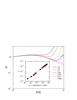
Figure 1: (Color online) Density decay ($t\rho(t)$) as a function of $\ln(t)$ for the CP on unweighted looped BA networks with $m=3$ of size $N=8\times 10^{7}$. The different curves correspond to $\lambda=1.2068,...,1.24$ (from bottom to top). Inset: Steady state density, showing agreement with HMF theory scaling. The full line shows a power-law fitting to the data points in the form $-0.36(5)x^{0.98(2)}$.

III.2 Unweighted BA trees

We now investigate the effect of a loop-less tree structure, again in the absence of weights. For small network sizes, $N\leq 10^{6}$, numerical results do not yield to simple interpretation. S-shaped density decay curves can be seen on log-log plots, in such a way that the location of the transition point cannot be clearly determined. This observation suggests the presence of corrections to scaling that could be larger than those predicted in the simple HMF analysis presented in Sec. A.1.1. In fact, as we increase the network size, a phase transition with power-laws (PL) seems to emerge, but the corrections became negligible only for network sizes $N>10^{7}$ nodes.

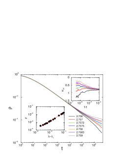
Figure 2: (Color online) Density decay as a function of time for the CP on unweighted tree BA networks of size $N=8\times 10^{7}$. The different plots correspond to $\lambda=2.756,...,2.759$ (from bottom to top). Right inset: The corresponding effective exponents from a local slopes analysis (increasing $\lambda=$ from bottom to top). Left inset: Steady state density with power-law fitting of the form (19) for parameters in opposite order (from top to bottom) as in the main graph.

In Fig. 2 we show the particle density decay on networks of size $N=8\times 10^{7}$ in a narrow scaling region around the critical point given by $2.756\leq\lambda\leq 2.759$. We have done a careful analysis of the steady-state, with $\rho$ leveling off to constant values, taking into account the effects of finite sizes. By assuming a critical transition (see left inset in Fig. 2) in the form

$$\rho(\infty)=A|\lambda-\lambda_{c}|^{\beta}\ ,$$ (19)

we obtain a critical point $\lambda_{c}=2.757(1)$ with $A=0.287$ and $\beta=1.20(5)$ by means of a least-squares fitting performed discarding the smallest values of $\lambda$. Note that this exponent $\beta\simeq 1.2$ is larger than the expected HMF result, an observation hinting towards a failure of the HMF theory for the CP on tree-like networks PhysRevE.78.011114 . The main plot of Fig. 2 depicts the decay in time of the particle density $\rho(t)$ for different values of $\lambda$ around the estimated critical point. The curves shown exhibit a decay exponent apparently varying with the value of $\lambda$ at very large times. In order to explore in more detail the decay of the density functions, we have computed an effective decay exponents, defined as the local slope of $\rho(t)$ as given by

$$\alpha_{\rm eff}(t)=-\frac{\ln[\rho(t)/\rho(t^{\prime})]}{\ln(t/t^{\prime})}\ ,$$ (20)

where $t$ and $t^{\prime}$ have been chosen in such a way that the discrete approximate of the derivative is sufficiently smooth, see right inset in Fig. 2. From this figure, we observe that the decay exponents are indeed different, smaller than the HMF prediction, which would lead to an effective exponent larger than one in a log-log plot. Moreover, the exponents thus computed are not well defined for all values of $\lambda$, since the plots of $\alpha_{\rm eff}(t)$ do not show in general well-defined plateaus except for very small regions at very large times.

The conclusion we draw from the analysis of non-weighted BA trees is that these network structures do not show evidence for the presence of explicit RR effects, but are compatible with a standard non-equilibrium phase transition. Evidences for RR effects, and in particular for a smeared transition, are however compelling in the case of weighted BA trees, as we will see below.

III.3 Weighted BA trees with multiplicative weights: WBAT-I model

We next investigate the possibility of inducing RR effects in the activity propagation of the CP by adding to the BA tree networks a weight structure wich will act against the “stronger gets stronger” behavior of BA models by suppressing the dominancy of strongly connected nodes.

In the first place, we consider the multiplicative weighting strategy defined by model WBAT-I. In this case, we have as a theoretical guideline for the behavior of the CP the results from the HMF analysis presented in Sec. II.2, which suggest a fully homogeneous mean-field behavior, with $\beta=\alpha=1$. We note that departures from this prediction are however not unexpected, given the tree-like and weighted structure of the network model under consideration.

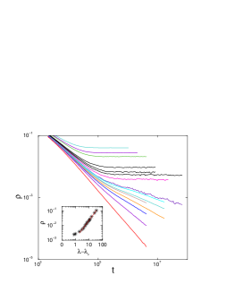
Figure 3: (Color online) Density decay as a function of time for the CP on weighted BA trees generated with the WBAT-I model with exponent $\nu=1.5$. Network size $N=10^{5}$. Different curves correspond to $\lambda=$ 160, 156, 154, 149, 148, 147, 146, 145, 144.7, 144.2, 144, 143.5, 143, 142, 140 (from top to bottom). Inset: Steady state density.

For a small weight exponent $\nu=1/2$ we find a phase transition at $\lambda_{c}=8.62(1)$, characterized by the mean-field type of density decay: $\rho(t)\propto 1/t$ (not shown) karsai:036116 . For larger values of $\nu$, however, generic, continuosly changing power-laws can be observed. In particular for $\nu=1.5$ simulations performed on networks of size $N=10^{5}$ suggest the presence of a GP as shown on Fig. 3. Considering the steady state value of the density, we can observe a very smooth approach to zero. A power-law fitting to the form $\rho=A|\lambda-\lambda_{c}|^{\beta}$ results is $\lambda_{c}=143(1)$ and $\beta=1.3(1)$, as shown in the inset of Fig. 3. The value of $\beta$ obtained in this fitting is again in disagreement with the HMF prediction from Sec. II.2.

We have also performed spreading simulations, starting from a very small initial seed of active sites odorbook . These simulations were performed on networks with $N=10^{5}$ nodes up to $t=4\times 10^{5}$ MC time steps. Besides the density $\rho(t)$, we measured the survival probability $P(t)$ marro1999npt , averaged over $10^{8}$ independent runs on $10^{3}$ different network configurations. As Fig. 4 shows, not only the density, but also the survival probability $P(t)$ curves exhibit slow, power-like behavior for times larger than $t>2000$. In the initial time region $t<1000$, both $P(t)$ and $\rho(t)$ decay exponentially.

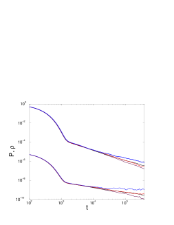
Figure 4: (Color online) Density decay as a function of time $\rho(t)$ (lowest branch curves) and survival probability $P(t)$ (highest branch curves) for seed simulations of the CP on weighted BA trees generated with the WBAT-I model with exponent $\nu=1.5$. Curves correspond to $\lambda=145,144,143,140$ (top to bottom for each branch). Network size $N=10^{5}$.

Simulations performed for larger network sizes suggest, however, that the apparent PLs observed in fact disappear in the thermodynamic limit of large network size. In Fig. 5 we plot the particle density decay as a function of time for $\lambda=140$ and $144$ corresponding to increasing network sizes from $N=10^{5}$ up to $N=10^{6}$. As can be seen from this plot, the apparent power laws, fitted by dashed lines, that can be observed for $N<10^{5}$, turn into saturation plateaus for $N=10^{6}$ at very late times.

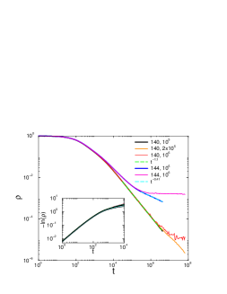
Figure 5: (Color online) Density decay as a function of time $\rho(t)$ for the CP on weighted BA trees with a multiplicative weighting scheme (WBAT-I) with exponent $\nu=1.5$. Plots correspond to two sets of $\lambda$ (upper branch: $\lambda=144$, lower branch $\lambda=140$) at different network sizes $N$. Dashed lines represent PL fittings. Inset: Initial time region of the same data, showing an stretched exponential behavior near the transition.

This observation suggests that what we are actually observing in the WBAT-I model is the tail behavior of a smeared transition Vojta , where the density has a constant nonzero value $\rho_{st}=\rho(\infty)$ in the long time limit and $\rho(t)$ approaches this in a PL manner, see Eq. (1). Additional evidence of this picture come from the analysis of the initial time decay of the particle density, with can be fitted to an stretched exponential of the form $\rho\propto\exp(t^{-0.91})$ (see inset on Fig. 5). This behavior is very close to an exponential decay. However, comparing with the CP with correlated disorder on regular lattices, at intermediate times of the smeared transition we should observe a stretched exponential of the form in Eq. (2). A value $d_{r}\gg z$ in Eq. (2) would fit to the observed behavior, an expectation that is quite reasonable in a random network with infinite topological dimensions.

The conclusion extracted from the analysis of this model is that the presence of a smeared phase transition is quite probable. A smeared transition can explain the saturation in the thermodynamic $N\to\infty$ limit, due to the presence of correlated subspaces of connected vertices of small degree, and correspondingly joined by relatively large weights. These subspaces play the role of RRs, that can remain active, leading to an initial stretched exponential dynamics crossing over to power-law for longer times DV05 .

In order to visualize the presence of these RRs, we have performed a percolation analysis stauffer94 ; ostojic06 ; 1742-5468-2012-02-P02008 of our WBAT-I networks. We consider a network of a given size $N$, and delete all the edges with a weight smaller than a threshold $\omega_{\mathrm{th}}$. For small values of $\omega_{\mathrm{th}}$, many edges remain in the system, and they form a connected network with a single cluster encompassing almost all the vertices in the network. When increasing the value of $\omega_{\mathrm{th}}$, the network breaks down into smaller subnetworks of connected edges, joined by weights larger than $\omega_{\mathrm{th}}$. The expectation in the latter case from standard percolation in networks is to observe the presence of a largest cluster (the giant component) with a size scaling with $N$, while the rest of the components should have a size scaling logarithmically with $N$ at most Newman2010 .

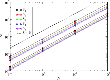
Figure 6: (Color online) Size $S_{i}$ of the $5$ largest clusters in a percolation analysis of the WBAT-I model with $\nu=1.5$ for $\omega_{\mathrm{th}}=100\omega_{\mathrm{min}}$ (hollow symbols) and $\omega_{\mathrm{th}}=1000\omega_{\mathrm{min}}$ (full symbols), where $\omega_{\mathrm{min}}$ is the minimum weight in the network. The size of all components grows linearly with network size $N$, and is therefore infinite in the thermodynamic limit.

In Fig. 6 we plot the average size (measured as the number of vertices) of the $5$ largest components corresponding to a given threshold $\omega_{\mathrm{th}}$. For the values of $\omega_{\mathrm{th}}$ considered, the networks break down in a number of components. However, the size of the largest ones grows linearly with the network size $N$, at odds with the expectations from a standard percolation transition. These clusters, which can become arbitrarily large in the thermodynamic limit, play the role of correlated RRs, sustaining independently activity and smearing down the phase transition.

This sort of analys allows also to explain why looped weighted networks do not exhibit RR effects. In this case (data not shown), the largest component scales again linearly with the network size, but the next largest components scale in size logarithmically. They thus become irrelevant in the thermodynamic limit and cannot sustain activity at very large times.

III.4 Weighted BA trees with age-dependent weights: WBAT-II model

We finally consider the behavior of the CP on weighted tree BA networks constructed with the age-dependent weighting scheme, defined by the model WBAT-II. In this case, the weights are anti-correlated with the degree, in opposition with the previous WBAT-I, in which large degree vertices had small weight, with small degree vertices had large weight. Here instead, weight is larger in edges connecting vertices with different degrees, while edges between vertices of similar degree have a small weight.

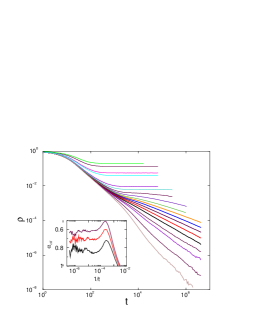
Figure 7: (Color online) Density decay as a function of time $\rho(t)$ for the CP on weighted BA trees with a age-dependent weighting scheme (WBAT-II) with exponent $x=2$. Network size $N=10^{5}$. Different curves correspond to $\lambda=$ 6.75, 6.8, 6.85, 6.87, 6.9, 6.92, 6.94, 6.96, 6.98, 7, 7.04, 7.1, 7,2, 7.4, 8.5, 9, 12, 15 (from top to bottom). Inset: Corresponding local slopes for $\lambda=6.9,6.92,6.94$ (from bottom to top).

Selecting an exponent for the weight strength $x=2$ and not very large network sizes, $N=10^{5}$, generic power-laws can be observed for a large range of $\lambda$ of values, as shown on Fig. 7, which exhibit a very strong similarity with those found in the multiplicative WBAT-I model, see Fig. 3. An analysis of the steady state density at large times in the region $6.8<\lambda<9$ can be fitted again to the canonical form $\rho=A|\lambda-\lambda_{c}|^{\beta}$, with $\beta=1.35(5)$, $A=0.02(5)$ and $\lambda_{c}=6.80(2)$. These values are again in discrepancy with HMF expectation, but this fact is altogether not surprising, since we do not have a proper HMF solution for this model, and we can only proceed to compare with the homogeneous result observed for the WBAT-I model. The inset in Fig. 7 shows the effective exponents $\alpha_{\rm eff}(t)$ as computed using the formula in Eq. (20). From the figure we observe the presence of reasonably large plateaus that confirm the presence of well-defined PLs with exponent varying with the value of $\lambda$.

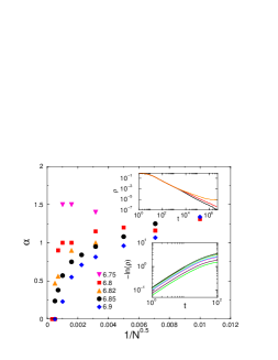
Figure 8: (Color online) Finite-size scaling analysis of the density decay exponent for $\lambda=6.75$ (triangles), $\lambda=6.8$ (boxes), $\lambda=6.82$ (triangles), $\lambda=6.85$ (bullets), $\lambda=6.9$ (rhombes) in the CP on weighted BA trees with a age-dependent weighting scheme (WBAT-II) with exponent $x=2$. Top inset: $\rho(t)$ for $\lambda=6.82$ ($N=10^{6}$, $N=4\times 10^{5}$, $N=10^{5}$ from top to bottom). Bottom inset: Initial time density near the transition.

Simulations over larger networks hint again towards the disappearance of the PLs observed in smaller network sizes (see top inset of Fig. 8). In Fig.8 we plot the value of the decay exponent for larger systems by performing a power-law regression in the last two decades of time. This seems to indicate that as a function of the network size for $\lambda>6.8$, the estimated exponent apparently tends to zero, suggesting the presence of an active phase in the thermodynamic limit. On the other hand, for $\lambda\leq 6.8$ the decay exponent does not change too much with $N$ and seems to stay $\alpha\geq 1$ up to the largest sizes $N=4\times 10^{6}$ we could reach by extensive simulations.

This kind of behavior can again be understood in terms of a smeared phase transition. Further evidence of this fact comes from the analysis of the initial decay of the activity density, which again can be fitted to a stretched exponential of the form $\rho\propto\exp(t^{-0.87(5)})$ (see bottom inset of Fig.8), in agreement with optimal fluctuation theory in an infinite dimensional network, Eq. (2). In this case, the corresponding correlated subspace will be formed by a subset of connected vertices with alternating small and large degree, and consequently joined by large weight edges, which would remain active in the thermodynamic limit giving rise to the characteristic RR effects observed in simulations. The nature of the RRs in this model can also be visualized by means of a percolation analysis.

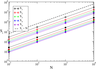
Figure 9: (Color online) Size $S_{i}$ of the $5$ largest clusters in a percolation analysis of the WBAT-II model with $x=2$ for $\omega_{\mathrm{th}}=100\omega_{\mathrm{min}}$ (hollow symbols) and $\omega_{\mathrm{th}}=1000\omega_{\mathrm{min}}$ (full symbols), where $\omega_{\mathrm{min}}$ is the minimum weight in the network. Curves in this last case have been shifted downwards for the sake of clarity.

In Fig. 9 we plot the average size of the $5$ largest components in percolation experiments for different values of the weight threshold $\omega_{\mathrm{th}}$. Again, all five scale linearly with network size, confirming their role as correlated RRs in the thermodynamic limit.

This sort of behavior is not exclusive of the value $x=2$ considered in the simulations above, but can also be observed for other values of $x$, see Fig. 10. The initial time dependence for $t<30$ MCS follows in this case $\rho\propto\exp(t^{-0.87(5)})$ (see right inset of Fig. 10).

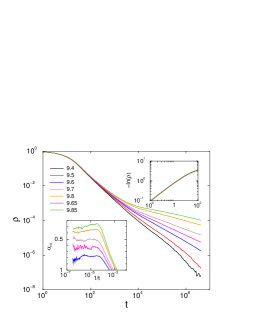
Figure 10: (Color online) Density decay as a function of time $\rho(t)$ for the CP on weighted BA trees with a age-dependent weighting scheme (WBAT-II) with exponent $x=3$. Different curves correspond to $\lambda=$ 9.4, 9.5, 9.6, 9.65, 9.7, 9.8, 9.85, (from bottom to top). Left inset: The corresponding effective exponents from a local slopes analysis for $\lambda=$ 9.6, 9.65, 9.7, 9.8, 9.85 (from bottom to top). Right inset: initial, stretched exponential behavior.

IV Conclusions

The heterogeneous and disordered pattern of connections in a complex network can induce considerable and surprising differences in dynamical processes running on top of them, as compared with their outcome on ordered or homogeneous systems. Building on recent results concerning the additional effects of intrinsic random, quenched disorder superimposed over a network structure, in this paper we have shown that topology-induced disorder can induce rare-region effects on the contact process. In particular, we have investigated the effects of a tree topology, in which no global loops are present in the network (there is a unique path between any two vertices) and of a correlated weight pattern assigned to the set of edges. Both elements have been show to induce a slowing down in dynamics as simple as diffusion. By means of large scale numerical simulations on tree-like weighted networks generated using the Barabási-Albert model, we have shown that a tree-like topology is not by itself enough to induce a slow dynamics or rare-region effects. However, the combined effects of a tree structure and a correlated weight pattern are indeed capable of triggering a very noticeable slow dynamics, which is compatible with the presence of rare-region effects. The two different weighting schemes we have considered for small system sizes suggested the appearance of Griffiths phases, characterized by a power-law dynamics of the activity and the survival probability above the clean critical point, with a varying decay exponents. More accurate simulations performed on larger network sizes indicate that, instead of true Griffiths phases, the behavior of the contact process on tree weighted networks is better explained in terms of a fully smeared transition, characterized by an initial time decay of the activity density with the form of an stretched exponential, whose presence can be understood by optimal fluctuation theory arguments applied on a network with infinite topological dimension. The smearing of the transition can be argued to be due to the presence of a correlated subspace of connected vertices, which are joined by large weight edges, playing the role of rare-regions and trapping activity at different large time scales.

To sum up, we have shown here that topological disorder is capable to induce rare-region effects on the contact process on complex networks. In the particular case we have considered (weighted tree networks), those rare-region effects translate in the smearing of the critical phase transition. Our work opens the path to a deeper investigation of this issue, focusing in particular on discovering those new topological ingredients which could induce fully-fledged Griffiths phase originating on topological grounds.

Appendix A Analytic solution of the HFM equations for WBAT-I model

In this section we develop the full HMF solution of the WBAT-I model on uncorrelated networks, sketched in Section II.2.

A.1 Steady state density

The starting point is Eq. (6), namely

$$\dot{\rho}_{k}(t)=-\rho_{k}(t)+\lambda[1-\rho_{k}(t)]\frac{k^{1-\nu}\rho(t)}{\langle{k^{1-\nu}}\rangle},$$ (21)

which, in the steady state regime, leads to the non-zero solution for the partial density of particles in vertices of degree $k$

$$\rho_{k}=\frac{\lambda k^{1-\nu}\rho/\langle{k^{1-\nu}}\rangle}{1+\lambda k^{1-\nu}\rho/\langle{k^{1-\nu}}\rangle}.$$ (22)

From this expression, $\rho$, the total density of particles, can be computed self-consistently, noticing that

$$\rho = \sum_{k}P(k)\rho_{k}=\sum_{k}P(k)\frac{\lambda k^{1-\nu}\rho/\langle{k^{1-\nu}}\rangle}{1+\lambda k^{1-\nu}\rho/\langle{k^{1-\nu}}\rangle}$$ (23)

$$= 2m^{2}\int_{m}^{\infty}\frac{\lambda k^{-2-\nu}\rho/\langle{k^{1-\nu}}\rangle}{1+\lambda k^{1-\nu}\rho/\langle{k^{1-\nu}}\rangle}\;dk,$$

where in the last expression we have used the degree distribution in its continuous degree form, $P(k)=2m^{2}k^{-3}$, and substituted sums by integrals. Performing the integral in Eq. (23) leads to an equation that can be solved to obtain $\rho$ as a function of $\lambda$. The form of this equation depends on the value of $\nu$. Let us consider separately the different cases.

A.1.1 $\nu=0$

In this case, Eq. (23) takes de form

$$\rho = 2m^{2}\int_{m}^{\infty}\frac{\lambda k^{-2}\rho/\langle{k}\rangle}{1+\lambda k\rho/\langle{k}\rangle}\;dk$$ (24)

$$= \lambda\rho\left[1-\frac{\lambda\rho}{2}\ln\left(\frac{2}{\lambda\rho}+1\right)\right],$$ (25)

where in the last expression we have used $\langle{k}\rangle=2m$. Eq. (25) provides an implicit equation for $\rho$ which, in the limit $\rho\to 0$, close to the critical point, leads to the explicit solution

$$\rho\simeq-\frac{2}{\lambda^{2}}\dfrac{\lambda-1}{\ln\left(\frac{\lambda-1}{\lambda}\right)},$$ (26)

which corresponds to the asymptotic behavior in Eq. (10).

A.1.2 $0<\nu<1$

In this case, performing the integral for $k$ in Eq. (23), we obtain the self-consistent equation

$$\rho=F\left[1,\frac{2}{1-\nu},1+\frac{2}{1-\nu},-\left(\frac{\lambda\rho m^{1-\nu}}{\langle{k^{1-\nu}}\rangle}\right)^{-1}\right],$$ (27)

where $F[a,b,c,z]$ is the Gauss hypergeometric function abramovitz . In order to evaluate the critical behavior of the density in the thermodynamic (infinite network size) lime, we can invert the previous expression using asymptotic expansion of the Gauss hypergeometric function abramovitz , namely

$$F\left[1,\alpha,1+\alpha,-\frac{1}{z}\right]=$$ (28)

$$z^{\alpha}\Gamma(\alpha+1)\Gamma\left(1-\alpha\right)+\alpha\sum_{n=1}^{\infty}(-1)^{n}\frac{z^{n}}{n-\alpha}.$$

For small $\rho$ (small $z$), since $2/(1-\nu)>2$ for $\nu>0$, the most relevant terms are $z$ and $z^{2}$. Thus, at leading order, the have

$$\rho\simeq\frac{2}{1+\nu}\frac{\lambda\rho m^{1-\nu}}{\langle{k^{1-\nu}}\rangle}-\frac{1}{\nu}\left(\frac{\lambda\rho m^{1-\nu}}{\langle{k^{1-\nu}}\rangle}\right)^{2}.$$ (29)

Using now the fact that, in the continuous degree approximation, $\langle{k^{1-\nu}}\rangle=2m^{1-\nu}/(1+\nu)$, we are led to the expression

$$\rho\simeq\frac{4\nu}{(1+\nu)^{2}\lambda^{2}}\left(\lambda-1\right),$$ (30)

recovering the asymptotic expression Eq. (11).

A.1.3 $\nu>1$

Now, the self-consistent equation for $\rho$ is

$$\rho=\lambda\rho\Gamma\left(\frac{2\nu}{\nu-1}\right)\tilde{F}\left[1,\frac{\nu+1}{\nu-1},1+\frac{\nu+1}{\nu-1},-\frac{\lambda m^{1-\nu}\rho}{\langle{k^{1-\nu}}\rangle}\right],$$ (31)

where $\tilde{F}[a,b,c,z]$ is the regularized Gauss hypergeometric function. Using the series expansion for small $z$ abramovitz

$$\Gamma(\alpha+1)\tilde{F}[1,\alpha,\alpha+1,-z]=\alpha\sum_{n=0}^{\infty}\frac{(-1)^{n}z^{n}}{n+\alpha},$$ (32)

the self-consistent equation at leading order in $\rho$ takes the form

$$\rho\simeq\lambda\rho\left[1-\frac{\nu-1}{\nu+1}\frac{\lambda m^{1-\nu}}{\langle{k^{1-\nu}}\rangle}\rho\right],$$ (33)

from where it follows that

$$\rho\simeq\frac{2}{(\nu-1)\lambda^{2}}(\lambda-1),$$ (34)

from which the scaling form Eq. (11) ensues.

A.2 Density decay at criticality

The decay of the particle density at criticality can be obtained from Eq. (12), namely

$$\dot{\rho}(t) = \sum_{k}P(k)\dot{\rho}_{k}(t)=-\frac{\rho(t)}{\langle{k}\rangle}\sum_{k}P(k)k\rho_{k}(t)$$ (35)

$$= m\rho(t)\int_{m}^{\infty}\frac{\lambda k^{-1-\nu}\rho(t)/\langle{k^{1-\nu}}\rangle}{1+\lambda k^{1-\nu}\rho(t)/\langle{k^{1-\nu}}\rangle}\;dk,$$

where in the last expression we have performed a quasi-stationary approximation, substituting $\rho_{k}(t)$ by the functional form in Eq. (30), and passed to the continuous degree approximation.

A.2.1 $\nu=0$

Eq. (35) takes the form

$$\dot{\rho}(t) = m\rho(t)\int_{m}^{\infty}\frac{\lambda k^{-1}\rho(t)/\langle{k}\rangle}{1+\lambda k\rho(t)/\langle{k}\rangle}\;dk$$ (36)

$$= -\frac{\rho(t)^{2}}{2}\ln\left(1+\frac{2}{\rho(t)}.\right)$$

This equation can be integrated, yielding

$$\mathrm{li}\left(1+\frac{2}{\rho(t)}\right)\simeq t,$$ (37)

where $\mathrm{li}(z)$ is the logarithmic integral function abramovitz . Using the asymptotic expansion $\mathrm{li}(z)\sim z/\ln(z)$ , we obtain the density decay in the large $t$ limit limit given by Eq. (13).

A.2.2 $\nu>0$

In the case $0<\nu<1$, integration of Eq. (35) leads to

$$\dot{\rho}(t)\simeq-\rho(t)F\left[1,\frac{1+\nu}{1-\nu},1+\frac{1+\nu}{1-\nu},-\left(\frac{\lambda\rho m^{1-\nu}}{\langle{k^{1-\nu}}\rangle}\right)^{-1}\right].$$ (38)

Expanding for small density, using Eq. (28), and noticing that at $(\nu+1)/(1-\nu)>1$, we have at leading order in $\rho$,

$$\dot{\rho}(t)\simeq-\frac{1+\nu}{\nu}\frac{\lambda m^{1-\nu}}{\langle{k^{1-\nu}}\rangle}\rho(t)^{2},$$ (39)

leading to the density decay, in the infinite network size limit, $\rho(t)\sim t^{-1}$.

An analogous calculation, implying the regularized Gauss hypergeometric functions, can be performed for $\nu>1$, leading to the same mean-field behavior for the density decay.

References

- (1) R. Albert and A.-L. Barabási, Rev. Mod. Phys. 74, 47 (2002)
- (2) S. N. Dorogovtsev and J. F. F. Mendes, Evolution of networks: From biological nets to the Internet and WWW (Oxford University Press, Oxford, 2003)
- (3) S. N. Dorogovtsev, A. V. Goltsev, and J. F. F. Mendes, Rev. Mod. Phys. 80, 1275 (2008)
- (4) A. Barrat, M. Barthélemy, and A. Vespignani, Dynamical Processes on Complex Networks (Cambridge University Press, Cambridge, 2008)
- (5) A.-L. Barabási and R. Albert, Science 286, 509 (1999)
- (6) T. E. Harris, Ann. Prob. 2, 969 (1974)
- (7) T. M. Liggett, Interacting Particle Systems (Springer-Verlag, New York, 1985)
- (8) J. Marro and R. Dickman, Nonequilibrium Phase Transitions in Lattice Models (Cambridge University Press, Cambridge, 1999)
- (9) G. Ódor, Universality in Nonequilibrium Lattice Systems (World Scientific, Singapore, 2008)
- (10) M. Henkel, H. Hinrichsen, and S. Lübeck, Non-equilibrium phase transition: Absorbing Phase Transitions (Springer Verlag, Netherlands, 2008)
- (11) C. Castellano and R. Pastor-Satorras, Phys. Rev. Lett. 96, 038701 (2006)
- (12) C. Castellano and R. Pastor-Satorras, Phys. Rev. Lett. 100, 148701 (2008)
- (13) S. C. Ferreira, R. S. Ferreira, and R. Pastor-Satorras, Phys. Rev. E 83, 066113 (2011)
- (14) S. C. Ferreira, R. S. Ferreira, C. Castellano, and R. Pastor-Satorras, Phys. Rev. E 84, 066102 (2011)
- (15) M. Boguñá, C. Castellano, and R. Pastor-Satorras, Phys. Rev. E 79, 036110 (2009)
- (16) J. L. Cardy, ed., Finite Size Scaling, Vol. 2 (North Holland, Amsterdam, 1988)
- (17) M. A. Muñoz, R. Juhász, C. Castellano, and G. Ódor, Phys. Rev. Lett. 105, 128701 (Sep 2010)
- (18) G. Ódor, R. Juhasz, C. Castellano, and M. A. Munoz, in Nonequilibrium Statistical Physics Today, Vol. 1332, edited by P. L. Garrido, J. Marro, and F. de los Santos (AIP, 2011) pp. 172–178
- (19) R. Juhász, G. Ódor, C. Castellano, and M. A. Muñoz, Phys. Rev. E 85, 066125 (2012)
- (20) R. B. Griffiths, Phys. Rev. Lett. 23, 17 (1969)
- (21) T. Vojta, Journal of Physics A: Mathematical and General 39, R143 (2006)
- (22) G. Bianconi, ArXiv e-prints(Apr. 2012), arXiv:1204.6282 [cond-mat.dis-nn]
- (23) A. B. Harris, Journal of Physics C: Solid State Physics 7, 1671 (1974)
- (24) A. J. Bray, Phys. Rev. Lett. 59, 586 (1987)
- (25) D. Dhar, M. Randeria, and J. P. Sethna, Europhys. Lett. 5, 485 (1988)
- (26) H. Rieger and A. P. Young, Phys. Rev. B 54, 3328 (1996)
- (27) D. S. Fisher, Phys. Rev. Lett. 69, 534 (1992)
- (28) F. Iglói and C. Monthus, Physics Reports 412, 277 (2005)
- (29) F. Vazquez, J. A. Bonachela, C. López, and M. A. Munoz, Phys. Rev. Lett. 106, 235702 (2011)
- (30) P. Erdös and P. Rényi, Acta. Math. Sci. Hung 12, 261 (1961)
- (31) D. J. Watts and S. H. Strogatz, Nature 393, 440 (1998)
- (32) A. Baronchelli, M. Catanzaro, and R. Pastor-Satorras, Phys. Rev. E 78, 011114 (2008)
- (33) A. Baronchelli and R. Pastor-Satorras, Phys. Rev. E 82, 011111 (2010)
- (34) S. Fortunato, Physics Reports 486, 75 (2010)
- (35) C. Castellano, V. Loreto, A. Barrat, F. Cecconi, and D. Parisi, Phys. Rev. E 71, 066107 (2005)
- (36) M. Catanzaro, M. Boguñá, and R. Pastor-Satorras, Phys. Rev. E 71, 027103 (2005)
- (37) R. Pastor-Satorras and A. Vespignani, Phys. Rev. Lett. 86, 3200 (2001)
- (38) R. Pastor-Satorras, A. Vázquez, and A. Vespignani, Phys. Rev. Lett. 87, 258701 (2001)
- (39) A. Barrat and R. Pastor-Satorras, Phys. Rev. E 71, 36127 (2005)
- (40) M. Boguñá and R. Pastor-Satorras, Phys. Rev. E 66, 047104 (2002)
- (41) M. Catanzaro, M. Boguñá, and R. Pastor-Satorras, Phys. Rev. E 71, 056104 (2005)
- (42) S. N. Dorogovtsev and J. F. F. Mendes, Advances in Physics 51, 1079 (2002)
- (43) J. D. Noh and S. W. Kim, Journal of the Korean Physical Society 48, S202 (2006)
- (44) L. Dall’Asta, A. Baronchelli, A. Barrat, and V. Loreto, Phys. Rev. E 74, 036105 (2006)
- (45) A. Baronchelli, C. Castellano, and R. Pastor-Satorras, Phys. Rev. E 83, 066117 (2011)
- (46) M. Karsai, R. Juhász, and F. Iglói, Phys. Rev. E 73, 036116 (2006)
- (47) M. Dickison and T. Vojta, Journal of Physics A: Mathematical and General 38, 1199 (2005)
- (48) D. Stauffer and A. Aharony, Introduction to Percolation Theory, 2nd ed. (Taylor & Francis, London, 1994)
- (49) S. Ostojic, E. Somfai, and B. Nienhuis, Nature 439, 828 (2006)
- (50) R. Pastor-Satorras and M.-C. Miguel, Journal of Statistical Mechanics: Theory and Experiment 2012, P02008 (2012), http://stacks.iop.org/1742-5468/2012/i=02/a=P02008
- (51) M. E. J. Newman, Networks: An introduction (Oxford University Press, Oxford, 2010)
- (52) M. Abramowitz and I. A. Stegun, Handbook of mathematical functions. (Dover, New York, 1972)