Characterizing dynamical transitions in bistable system using non-equilibrium measurement of work

Abstract

We show how Jarzynski relation can be exploited to analyze the nature of order-disorder and a bifurcation type dynamical transition in terms of a response function derived on the basis of work distribution over non-equilibrium paths between two thermalized states. The validity of the response function extends over linear as well as nonlinear regime and far from equilibrium situations.

I Introduction

Advancement of micromanipulation techniques has opened up the new possibility of estimating equilibrium thermodynamic quantities from non-equilibrium measurements in recent yearsjar1 ; jar2 ; crooks ; wang ; Carbe ; Liphardt ; hummer ; bussi ; hatano ; speck ; rito . The experiments with pulling forces of piconewton magnitude on RNA moleculesLiphardt ; hummer and dragging colloidal particles in a fluidwang ; Carbe have made it possible to measure the probability distribution of work exerted on a system. Since the relaxation time of the system concerned in these experiments is too long compared to the time scale over which the non-equilibrium measurements are made, work fluctuations over non-equilibrium irreversible paths play an important role in estimating the free energy difference between the thermalized initial and final states of the system. This is reflected in celebrated Jarzynski relationjar1 ; jar2 which relates the work distribution and the Helmholtz free energy difference $\Delta F$ as

$$e^{-\beta\Delta F}=\langle e^{-\beta W}\rangle$$ (1)

where the averaging on the exponential function of the work variable $W$ has been carried out with work distribution $P(W)$, $\beta$ being $1/k_{B}T$ with $k_{B}$ and $T$ denoting the Boltzmann constant and temperature, respectively. Central to these studies are several results, e. g., the so-called fluctuation theorems expressing transient violation of second law of thermodynamics where the systems in question are driven arbitrarily far from equilibrium.

The probability distribution of work $P(W,t)$ done on a system by manipulating an external agency or force is followed over irreversible paths for a given protocol. As free energy is the key quantity for carrying thermodynamic information and for description of transition between different states, it is apparent that, by virtue of Jarzynski equalityjar1 ; jar2 it is possible to probe the signature of dynamical transition in the behaviour of work distribution. The problem is non-trivial since for a nonequilibrium system, in general, free energy functional can not be defined. This, in consequence, raises difficulty in constructing a response function directly in terms of free energy and its derivatives with respect to suitable parameters of the system in the spirit of what is done in equilibrium phase transition. This difficulty, however, can be overcome with the help of Jarzynski equality by probing work fluctuations on the system even far from equilibrium. The object of the present paper is to examine this issue and to look for the response function which is characteristic of the dynamical system under study and is derivable from work distribution. In what follows we use a model potential to explore the order-disorder transition as well as a transition arising out of bifurcation of the response function in terms of the time evolution of work distribution function. The dynamics is described by a Langevin equation which appropriately takes care of the variation of the potential parameter in inducing transition from an unimodal to bimodal characterpkg2 ; ff5 . The implication of the results are elaborated.

II The model and the equilibrium description

Consider a Brownian particle in a thermal bath at temperature $T$ and subjected to an external potential force. The governing Langevin equation is given by

$$\dot{x} = p$$ (2a)

$$\dot{p} = -\gamma p-V^{\prime}(x,t)+\Gamma(t)$$ (2b)

where $V(x,t)$ is the external potential and $\gamma$ is the dissipation constant. $x$ and $p$ denote the coordinate and the momentum of the particle, respectively. Thermal fluctuations $\Gamma(t)$ of the bath are modeled by Gaussian, zero mean and delta correlated noise

$$\langle\Gamma(t)\rangle = 0$$ (3a)

$$\langle\Gamma(t)\Gamma(t^{\prime})\rangle = 2D\delta(t-t^{\prime})$$ (3b)

where $D=\gamma k_{B}T$ is the strength of the noise. We make use of potential $V(x,t)$ of the following form

$$V(x,t)=-\frac{1}{2}\left\{a-\lambda(t)a_{0}\right\}x^{2}+\frac{1}{4}bx^{4}$$ (4)

where $a,\;a_{0},\;b$ are the potential parameters and $\lambda(t)$ is a switching parameter. We first allow the system to reach an equilibrium with the heat bath at temperature $T$ and then switch on the parameter, infinitely slowly from an initial state $\lambda=0$ to a final state $\lambda=1$. The model has been explored in the literature under diverse conditions ^13,14. At the initial state the potential is bistable with two minima at $x=\pm\sqrt{{a/b}}$ and one maximum at $x=0$. The corresponding distribution function is bimodal in position coordinate($x$)

$$P_{0}(x,p)\sim\xi(p)\exp{\left[\frac{\;1/2ax^{2}-1/4\;bx^{4}}{D}\right]}$$ (5)

where $\xi(p)=\exp{(-p^{2}/2K_{B}T)}$At the final state, $\lambda=1$, for $a>a_{0}$ the potential is also bistable with two shifted minima at $x=\pm\sqrt{{(a-a_{0})/b}}$ and one maximum at $x=0$. For $a=a_{0}$, the potential contains only $x^{4}$ term and the corresponding distribution function is unimodal as follows;

$$P_{f}(x,p)\sim\xi(p)\exp{\left[\frac{-1/4\;bx^{4}}{D}\right]}$$ (6)

So the switching process induces a transition of the distribution function from bimodal($\lambda=0$) to unimodal one($\lambda=1$). This is depicted in Fig.1(a,b). Fig.1(a) also includes the case for $a<a_{0}$ for $\lambda=1$. The potential well is steeper compared to previous case ($V(x)=bx^{4}$). The corresponding probability distribution is also shown in Fig.1(b).

Figure 1: A schematic illustration for switching of (a) the potential energy for different values of the parameter $\lambda$ around the transition point for $(a-\lambda(t)a_{0})=a$ corresponding to $V_{0}$ ($\lambda=0$, solid line), $(a-\lambda(t)a_{0})=a/2$ corresponding to $V_{t}$ ($\lambda=1/2,$, dashed line, $(a-\lambda(t)a_{0})=0$ corresponding to $V_{f}$ ($\lambda=1$, dotted line), and dash-dot line present the case $(a-\lambda(t)a_{0})<0$ (b) distribution function for the corresponding cases. In all the illustrations $a=a_{0}$.

As both the initial and final states are in equilibrium the free energies of these states are given by

$$F_{0}=-k_{B}T\ln{Q_{0}}\;;\;\;\;\;\;\;\;\;\;\;\;F_{f}=-k_{B}T\ln{Q_{f}}$$

respectively, where $Q$ denotes the partition function. These are given by the following expressions

$$Q_{0} = \int_{-\infty}^{+\infty}dp\;dx\;\exp{\left[-\frac{(1/2)\;p^{2}-(1/2)\;ax^{2}+(1/4)\;bx^{4}}{k_{B}T}\right]}$$ (7)

$$Q_{f} = \int_{-\infty}^{+\infty}dp\;dx\;\exp{\left[-\frac{(1/2)\;p^{2}-(1/2)\;(a-a_{0})x^{2}+(1/4)\;bx^{4}}{k_{B}T}\right]}$$ (8)

respectively. By numerical integration one can easily find out the change in free energy for arbitrary values of $a_{0}$.

$$\Delta F=F_{f}-F_{0}=-k_{B}T\ln{\left(\frac{Q_{f}}{Q_{0}}\right)}$$ (9)

The linear coefficient $a_{0}$ serves here as the constant parameter of the system. $a_{0}$ governs the nature of ”phase” as a region of space in which the free energy function is analytical and continuous. The dynamical transition is associated with the crossing of boundary between the two regions. To understand the nature of transition it is therefore worthwhile to look for any discontinuity or irregularity of the first and second derivatives with respect to the control parameter at the boundary. With this in mind we, in Fig 2(a), present the variation of free energy change as a function of $a_{0}$ at different temperature. In the spirit of traditional way of deriving thermodynamic information and characterizing equilibrium phase transition, one may now define an extensive variable, an order parameter type quantity as, $-\left(\frac{\partial\Delta F}{\partial a_{0}}\right)_{T}$ analogous to magnetization $M$ associated with the free energy of a magnetic system as $M=-\left(\frac{\partial F}{\partial H}\right)_{T}$ (therefore role of magnetic field $H$ is played by $a_{0}$). Pushing the analogy a bit further we define a response function as a second order derivative with respect to $a_{0}$ as

$$\Psi=-\frac{\partial^{2}\Delta F}{\partial a_{0}^{2}}$$ (10)

Figure 2: (a) Variation of free energy change with $a_{0}$ at different temperature, (b)variation of $\frac{\partial\Delta F}{\partial a_{0}}$ with $a_{0}$ at different temperature, for the parameter set $a=0.5,\;b=0.005,\;K_{B}=1$.

Clearly the above expression is analogous to the magnetic susceptibility which measures the variation of magnetization due to the change of the external field. The magnetic susceptibility is related to the second order derivative of free energy as $\chi=-\left(\frac{\partial^{2}F}{\partial H^{2}}\right)$. In Fig.2 (b) we depict the first order derivative of free energy change with respect to $a_{0}$ at different temperature. While no discontinuity or singularity is observed in the curve, the behaviour of response function (2.9) as shown in Fig.3 is markedly different.

Figure 3: Response function vs $a_{0}$ plot at different temperature for the parameter set $a=0.5,\;b=0.005,\;K_{B}=1$ (using Eq.(2.9)).

The response function gradually increases to a maximum followed by a sharp fall at around $a_{0}=a$. This type of variation of response function with $a_{0}$ illustrates two types of dynamical transitionsancho . (i) The first one corresponds to a transition from an ordered state to a dis-ordered state for $\Delta V=k_{B}T$. The barrier height of the potential ($\Delta V$) is $(a-a_{0})^{2}/4b$. So with increasing value of $a_{0}$ ($a_{0}>0$) the barrier height gradually decreases. At $a_{0}=a-2\sqrt{bk_{B}T}$, the barrier height is double to average kinetic energy of the particle. The response function($\Psi$) at this point shows a maximum, presumably indicating the existence of a disordering transition. The existence of the transition point can be physically explained as follows: Whenever the value of average kinetic energy crosses half of the barrier height the particles start moving more randomly between two wells in a way as if they (relatively large number of the particles) feel no barrier between them. This is due to the fact that in this temperature domain the distribution of kinetic energy gains a broad range. Here lies a valid reason for existence a relation between barrier height and kinetic energy in the transition region. As expected with the increase in temperature the transition point shifts towards the origin. (ii) The second type of transition is due to a change of distribution function as reflected in Fig.3 by a very sharp change(bifurcation) in the response function at $a_{0}=a$. This transition is intrinsically different in nature from the previous one which can be controlled by adjusting the temperature of the system. In the later case, however, the temperature has no significant influence.

III Jarzynski relation and work distribution for transition in nonequilibrium system

For infinitely slow switching($\lambda=0$ to $\lambda=1$) of the potential parameter(Eq.(4)), the system remains in quasistatic equilibrium with the reservoir throughout the switching process and the total work performed on the system will be equal the Helmholtz free energy difference between initial and final state states ($W=\Delta F$). If the switching process occurs with a finite rate, the total work spent in changing the state of a system will depend on the microscopic initial conditions of the system and the reservoir and obey the following inequality

$$\langle W\rangle>\Delta F$$

In this case, the time evolution of the system of interest as described earlier(Eq.(2a,b)) is governed by a stochastic phase space trajectory, which depends on the externally imposed time dependence of the switching parameter $\lambda(t)$. For the present purpose we consider a constant switching rate, $\dot{\lambda}=1/t_{f}$ ($t_{f}$ is the final time starting from $t=0$). With this time dependence of switching parameter the total work performed along one particular trajectory ($z(t)$) up to time $t$ is given by

$$W[z(t),t]=\int_{0}^{t}dt\;\left(\frac{1}{t_{f}}\right)\frac{\partial V}{\partial\lambda}(z(t))$$ (11)

The equation for time evolution for work is given by

$$\dot{W}=\frac{1}{t_{f}}\frac{\partial V}{\partial\lambda}(z(t))$$ (12)

Although the equation of motion for $W$ does not have an explicit dependence on noise it is stochastic through its dependence on phase space variables.

Figure 4: Plot of work distribution function for different values of switching rate for the parameter set $a=0.5,\;b=0.005,\;T=1.0,\;K_{B}=1\;{\rm and}\;\gamma=2.5$.

Before we proceed to analyze the essential features of dynamical transition in terms of the work done we first numerically simulate the stochastic coupled equations Eq(2a,b) along with the equation for work (12) simultaneously using standard Heun’s algorithm and calculate the distribution of work, average work, higher moments of work. This allows us to calculate the free energy change from Jarzynski relation as a non-equilibrium estimate. We use in our numerical simulation a slowly varying time dependent quantity $\lambda(t)$, with switching rate $\dot{\lambda}\sim 10^{-5}-10^{-6}$. A very small time step($\Delta t$) of $0.01$ for numerical integration has been used. For the initial conditions we have assumed that at $t=0$ all the particles are in the potential minimum at $x=\sqrt{a/b}$ with zero velocity. In our simulation, we first allow the system to equilibrate with the reservoir to smooth out the effects due to the influence of initial conditions and transient processes. After the equilibration process we switch on the parameter ($\lambda(t)$). In calculation of average and higher moments the averaging is done over 20,000 trajectories. The parametric dependence of stochastic trajectory takes care of energy balancesuzki for Langevin dynamics when work is calculated in terms of Eq.(3.1).

Figure 5: In this figure we have depicted work distribution function for different switching rate with corresponding Gaussian fitting curve. The parameter set: $a=0.5,\;b=0.005,\;T=1.0,\;K_{B}=1\;{\rm and}\;\gamma=2.5$.

We first calculate the work distribution, average work and work fluctuation for different switching rate. This is shown in Fig.4 and Table-I. As revealed by Fig.4 the distribution is nearly Gaussian for low switching rate centering around $\langle W\rangle$, which is larger than free energy change( $\Delta F$) (The vertical dotted line does not indicate the center of the distribution but shown only to highlight the portion at which $W$ matches $\Delta F$). With decreasing switching rate the center of the distribution is shifted towards the line of free energy change, $\Delta F=11.862536$ (average work done tends to be equal to the free energy change along with the decrease of width of distribution). The distribution function $P(W)$ tends to $P(W)\rightarrow\delta(\langle W\rangle-\Delta F)$ . In Fig.5 we have depicted the work distribution function along with corresponding Gaussian fitting curve for relatively larger switching rate ($\dot{\lambda}>10^{-5}$). From Fig.5 it is apparent that the work distribution function is not a Gaussian for arbitrary switching rate. One observes that the higher order cumulants are important. (The distribution will be a Gaussian only if the switching speed is very slow for which the higher order cumulants effectively zero). We present Table-I depicting the variation of average work and width of the work distribution with switching rate.

Table 1: The table presents nonequilibrium estimates of average work and width of work distribution for different values of switching rate for $a=0.5,\;b=0.005,\;T=1.0,\;K_{B}=1\;{\rm and}\;\gamma=2.5$.

Switching rate	$\langle W\rangle$	$\Delta W^{2}$ ($=\langle W^{2}\rangle-\langle W\rangle^{2}$)
$9.375\times 10^{-5}$ $3.125\times 10^{-5}$ $9.375\times 10^{-6}$ $3.125\times 10^{-6}$	11.889384 11.878023 11.870123 11.863661	0.049791 0.032513 0.017320 0.002563

To verify the Jarzynski relation we numerically estimate the quantity $\langle e^{-W/k_{B}T}\rangle$. For a comparison of this result with the analytically calculated free energy we present a data Table-II for different values of $a_{0}$. The calculated free energy change using Jarzynski relation

$$\Delta F=-k_{B}T\ln{\left(\langle e^{-W/k_{B}T}\rangle\right)}$$ (13)

matches almost exactly (absolute difference is less then $0.01$ $\%$).

Table 2: The table presents a comparison of free energy change calculated analytically (equilibrium estimate) and numerically using Jarzynski relation (non-equilibrium estimate) for different values of $a_{0}$. The other parameter set for this data table are $a=0.5,\;b=0.005,\;T=1.5,\;K_{B}=1,\;\gamma=2.5$, and Switching rate $=5\times 10^{-6}$.

$a_{0}$	$\Delta F$ (using Eq.(2.8), equilibrium estimate )	$\langle W\rangle$	$\Delta W^{2}$	$\Delta F$ (using Jarzynski relation Eq.(13) non-equilibrium estimate)	$\Delta F=\langle W\rangle-\frac{1}{2}\frac{\Delta W^{2}}{k_{B}T}$ (fluctuation-dissipation estimate)
0.46 0.47 0.48 0.49 0.50 0.51 0.52 0.53 0.54	11.452822 11.522062 11.58799 11.650821 11.710751 11.767964 11.822633 11.874918 11.924969	11.456438 11.525216 11.592910 11.655346 11.714050 11.772241 11.827798 11.878662 11.929216	0.011571 0.0119362 0.012375 0.012639 0.012955 0.013103 0.013666 0.014022 0.014020	11.452579 11.521237 11.588780 11.651129 11.709732 11.767872 11.823242 11.873984 11.924543	11.452581 11.521238 11.588785 11.651133 11.707931 11.767873 11.823243 11.873988 11.924542

As revealed by the data set of Table-II the following relation for the free energy change with work holds very good as a fluctuation-dissipation estimate

$$\Delta F=\langle W\rangle-\frac{1}{2k_{B}T}\left\{\langle W^{2}\rangle-\langle W\rangle^{2}\right\}$$ (14)

the dissipative work being equal to the width of the distribution of work,

$$w_{diss}=\frac{1}{2k_{B}T}\left\{\langle W^{2}\rangle-\langle W\rangle^{2}\right\}$$ (15)

A final remark on Table-II may be in order. Since the work fluctuations have been determined with the help of Langevin dynamics with a Gaussian noise, fluctuation-dissipation estimate in Eq.(3.4) matches well with free energy change. For a different protocol for following the trajectory or for higher switching rate the deviation from linear response is expected where non-Gaussian distributions of work make their presence felt. The latter aspect is evident in Fig.5.

IV Study of dynamical transition by work fluctuation and response function

We recall that a system out of equilibrium can not, in principle, be described by free energy and therefore no free energy functional or partition function methodology can be applied for non-equilibrium system for classification of dynamical transition. Guided by a close analogy with equilibrium phase transition in Sec.II we have identified an appropriate response function $\Psi$ for description of dynamical transition. Analysis of Sec.III on the other hand suggests that by virtue of Jarzynski relation one can relate the free energy change (rather than free energy itself) between two thermodynamic states to microscopic work fluctuation for non-equilibrium paths connecting these states. The question is, can we bypass the description based on free energy change as done in Sec.II to compute the response function $\Psi$ directly from work fluctuation and recover the features of non-equilibrium dynamical transition. To this end we now proceed to calculate the response function $\Psi$ in terms of the work performed using Eq.(14) and Eq.(15) as follows;

$$\Psi=-\frac{\partial^{2}\Delta F}{\partial a_{0}^{2}}=-\frac{\partial^{2}\langle W\rangle}{\partial a_{0}^{2}}+\frac{\partial^{2}w_{diss}}{\partial a_{0}^{2}}$$ (16)

From Eq.(11) and (4) the work performed for the switching process along a particular trajectory is given by

$$W[z(t)]=\int_{0}^{t_{f}}dt\;\left(\frac{1}{t_{f}}\right)\frac{1}{2}a_{0}\;x^{2}$$ (17)

As revealed by the above expression the work performed is a linear function of $a_{0}$ only if the process $x(t)$ is independent of control parameter($a_{0}$). In this situation we have

$$\frac{\partial\langle W\rangle}{\partial a_{0}}=\frac{\langle W\rangle}{a_{0}}\;;\;\;\;\;\;\;\;\frac{\partial^{2}\langle W\rangle}{\partial a_{0}^{2}}=0$$ (18)

With the help of the Eq.(18) the response function can be expressed in a simplified form as

$$\Psi=\frac{1}{a_{0}^{2}}\frac{\langle W^{2}\rangle-\langle W\rangle^{2}}{2k_{B}T}$$ (19)

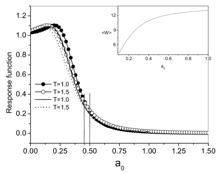
Figure 6: The solid and dotted lines present the variation of response function without dissipative work as a function of $a_{0}$ for different values of temperature. The lines containing hollow and solid circles present the variation of response function with inclusion of dissipative work as a function of $a_{0}$ for different values of temperature. The parameter set used $a=0.5,\;b=0.005,\;\gamma=2.5\;K_{B}=1$ . The inset plot presents the variation of work as a function $a_{0}$ for the same parameter set as in the main figure but for $T=1.0$, Switching rate $=10^{-5}$.

The response function is thus related to dissipative work. The above expression for response function has a close similarity to other linear response functions, as for example, heat capacity $C_{v}=\frac{\langle E^{2}\rangle-\langle E\rangle^{2}}{2k_{B}T}$, magnetic susceptibility $\chi=\frac{\langle M^{2}\rangle-\langle M\rangle^{2}}{2k_{B}T}$, where $E$ and $M$ denote internal energy and magnetization, respectively. A difference between linear response functions and $\Psi$, however, is noteworthy¹¹. Since $E$ and $M$ are well-defined equilibrium properties of a macroscopic system in the thermodynamic limit while $W$ by its very nature corresponds a quantity defined for non-equilibrium paths, heat capacity and susceptibility are typical static response function in contrast to the non-equilibrium response $\Psi$.

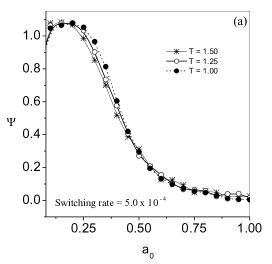
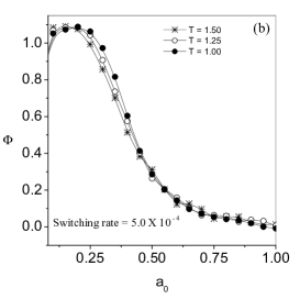
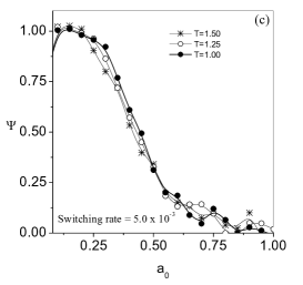
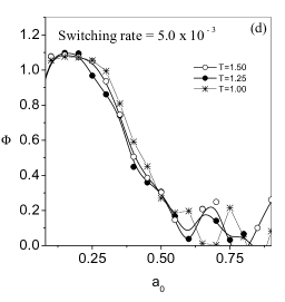
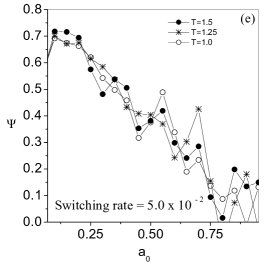
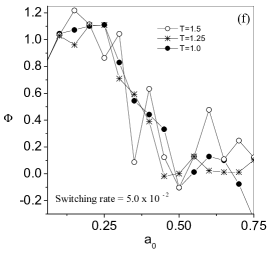
Figure 7: The subfigures (a, c, e) present the variation of response function $\Psi$ with $a_{0}$ and the subfigures (b, d, f) present the variation of $\Phi=-\frac{\partial^{2}\langle W\rangle}{\partial a_{0}^{2}}$ with $a_{0}$ depicting dynamical transition for different switching rate. The parameter set used $a=0.5,\;b=0.005,\;\gamma=2.5\;K_{B}=1$.

In the present problem the work, however, is not a linear function of $a_{0}$. This is due to the fact that $a_{0}$ bears an implicit dependence on $x(t)$. The non-equilibrium estimation of $\langle W\rangle$ shows that,in general, it is a nonlinear function of $a_{0}$, as depicted in the inset of plot Fig.6. $\langle W\rangle$ behaves linearly only for small values of $a_{0}$. The second derivative of the average work also predicts two transition points as discussed in Sec.II. But the transition points are slightly shifted from original position of the transition point (this is depicted in Fig.6). It should however be emphasized that although the second order variation of average work predicts only the approximate transition point, the inclusion of the contribution due to dissipative work gives an accurate estimate of the transition points as shown in Fig.6 (the plots containing solid and hollow circle).

In order to check the dependence of response function on switching rate we present the variation of response function as a function of $a_{0}$ for different switching rate in the Fig.7 (a,c,e). One observes that fluctuations become larger for higher switching rate. It may, however, be checked that the nature of the variation of response function with $a_{0}$ remains same. Although the nature of variation of the response function indicates two types of dynamical transition for arbitrary switching rate, but it is difficult to point out the transition points for higher switching rate due to fluctuating nature of $\Psi$. Moreover in order to figure out the relative contribution of second derivative of average work, i. e., $-\frac{\partial^{2}\langle W\rangle}{\partial a_{0}^{2}}$ and that of dissipative work $-\frac{\partial^{2}W_{diss}}{\partial a_{0}^{2}}$ in response function we present the subfigures of Fig.7 as a pair (a,b), (c,d) and (e,f). While Figs.7(a,c,e) represent variation of response function including dissipative work, Figs.7(b,d,f) represent the cases without dissipative work. From these figures it is clear that one can identify the dynamical transitions by calculating only second derivative of average work, i. e., $\frac{\partial^{2}\langle W\rangle}{\partial a_{0}^{2}}$. Thus the nature of the variation of response functions derived from work fluctuations are practically independent of any pulling speed which is a correct reflection of Fig.3. The response function(4.1) or (4.4) is completely determined by the stochastic equations (2.1) and (3.1) of the dynamical system independent of free energy description of the system in the thermodynamic limit.

V Conclusion

Analysis of transition between two equilibrium states is traditionally based on free energy change in a system with respect to a relevant parameter and linear response function is related to fluctuation of the order parameter around equilibrium. In view of the fact that free energy remains undefined for non-equilibrium systems, any analysis of response function on the basis of similar argument is untenable. However as Jarzynski equality is related to free energy change with work fluctuations during the passage of the system over many non-equilibrium paths when the parameter of the potential is varied, it is possible to look for the signature of dynamical transition in the behaviour of work fluctuations. The key quantity is the response function, which exhibits a characteristic behaviour of the system itself with no limitation imposed by near-equilibrium condition. Based on a model system we have examined two types of transition, e., g., order-disorder type and a bifurcation type which can be differentiated by their thermal behaviour around the transition points. As the Jarzynski relation and the related fluctuation theorems are valid even far from equilibrium situations, the response functions derived from work fluctuations, we believe, have a wider range of applicability, i., e., beyond linear regime and the results obtained for this simple system may be extended to explore more complex issues.

- (1) C. Jarzynski, Phys. Rev. Lett. 78, 2690 (1997); J. Stat. Mech.: Theory Exp., P09005 (2004).
- (2) C. Jarzynski, Phys. Rev. E 56, 5018 (1997).
- (3) G. E. Crooks, Phys. Rev. E 60, 2721 (1999).
- (4) G. M. Wang, E. M. Sevick, E. Mittag, D. J. Searles, and D. J. Evans, Phys. Rev. Lett. 89, 050601 (2002).
- (5) D. M. Carberry, J. C. Reid, G. M. Wang, E. M. Sevick, D. J. Searles, and D. J. Evans, Phys. Rev. Lett. 92, 140601 (2004).
- (6) J. Liphardt, S. Dumont, S. B. Smith, I. Tinoco and C. Bustamente, Science 296, 1832 (2002).
- (7) G. Hummer and A. Szabo, PNAS 98, 3658 (2001).
- (8) G. Bussi, A. Laio, and M. Parrinello, Phys. Rev. Letts 96, 090601 (2006).
- (9) T. Hatano, Phys. Rev. E, 60 R5017 (1999).
- (10) T. Speck and U. Seifert, Phys. Rev. E 70, 066112 (2004).
- (11) F. Ritort; Poincare Seminar, 2, 193 (2003) and references therein.
- (12) J. García-Ojalvo, and J.M. Sancho, Noise in Spatially Extended Systems (Springer-Verlag, New York, 1999).
- (13) P. K. Ghosh, D. Barik and D. S. Ray, Phys. Lett. A 342 12 (2005).
- (14) M. Borromeo and F. Marchesoni, Europhys Lett 68, 784 (2004); M. Marchi et al. Phys. Rev. E 54, 3479 (1996).
- (15) D. Suzuki et al., Phys. Rev. E 68, 021906 (2003).