Time-Resolved Magnetic Relaxation of a Nanomagnet on Subnanosecond Time Scales
Abstract
We present a two-current-pulse temporal correlation experiment to study the intrinsic subnanosecond nonequilibrium magnetic dynamics of a nanomagnet during and following a pulse excitation. This method is applied to a model spin-transfer system, a spin valve nanopillar with perpendicular magnetic anisotropy. Two-pulses separated by a short delay ( ps) are shown to lead to the same switching probability as a single pulse with a duration that depends on the delay. This demonstrates a remarkable symmetry between magnetic excitation and relaxation and provides a direct measurement of the magnetic relaxation time. The results are consistent with a simple finite temperature Fokker-Planck macrospin model of the dynamics, suggesting more coherent magnetization dynamics in this short time nonequilibrium limit than near equilibrium.
The control of magnetization on short timescales has become an area of intense research and many methods are used to excite a magnetic system, including spin-currents Koch et al. (2004); Garzon et al. (2008), magnetic fields Schumacher et al. (2003) and optical pulses Vaterlaus et al. (1991); Beaurepaire et al. (1996). It also has recently become possible to drive individual nanometer scale magnetic elements far from equilibrium using spin-currents and probe their dynamical response. However, most electronic transport studies focus on the excitation during the drive pulses Devolder et al. (2008); Cui et al. (2010). Less is known about the relaxation processes following a pulse excitation. Yet, this is very important for fundamental and practical reasons. First, the time scales of the relaxation far from equilibrium are not known and may differ from those determined in experiments that probe low amplitude magnetic excitations, such as ferromagnetic resonance. Second, these time scales determine the speed at which nanomagnets can be written and read in magnetic memories, including in spin-transfer torque magnetic random access memories (STT-MRAM).
It is now well known that spin-polarized currents and spin-transfer torques (STTs) can reverse the direction of the magnetization on subnanosecond timescales Koch et al. (2004); Bedau et al. (2010a). In fact, many experimental methods have been developed to study spin-transfer switching in both spin valves and magnetic tunnel junctions (MTJs). While MTJs are promising for applications because of their large magnetoresistive (MR) readout signals (%), all-metallic spin valves permit one to apply much larger currents and thus can be driven farther away from equilibrium. Direct single-shot time-resolved electrical measurements have been carried out in MTJs Devolder et al. (2008); Cui et al. (2010), but have not been reported in spin valve nanopillars, because of their low impedance and small magnetoresistance (MR) (%), which results in their switching signals being to small for nanosecond measurements. Further, time-resolved STT measurements are insensitive to the magnetization dynamics after the excitation, as the excitation current is the source of the electrical readout signal. Therefore, to time-resolve the relaxation dynamics, a different experimental method is needed.
In this paper we present an all-electrical two-pulse correlation method that yields quantitative information on the form and timescales of magnetic excitation and relaxation, with 50 ps time resolution. This method is applied to a model spin-transfer system, a spin valve nanopillar with perpendicular magnetic anisotropy. Two-pulses separated by a short delay ( ps) are shown to lead to the same switching probability as a single pulse with a duration that depends on the delay–demonstrating a remarkable symmetry between magnetic excitation and relaxation–and providing a direct measurement of the magnetic relaxation time. The observed symmetry is shown to be consistent with a finite temperature macrospin model.
The system we studied has two stable magnetic states and , which are nearly degenerate in equilibrium. We are interested in how the system relaxes to these states after being excited by a spin-polarized current. The basic idea of our method is to compare the switching probability of two pulses separated by a delay much longer than the magnetic relaxation time to that of a composite pulse, i.e. two pulses separated by a short delay. With a composite pulse, the first pulse alters the magnetic state on a time scale that changes the dynamics excited by the second pulse. By choosing the amplitudes and polarities of the first and second pulse we can study different aspects of the relaxation processes. For example, to study the relaxation back to the initial state (i.e. state ) after a pulse, we can apply two pulses with identical polarities that both would be of the appropriate polarity to switch the sample from state to . If the delay is much longer than the relaxation time , the two pulses can be considered to be independent events and the total probability of switching from state to state is:
Here , and are the switching probabilities from state to for the first, the second and for both pulses combined and we have assumed no reverse switching during the measurement, i.e. . If is within the relaxation time of the system, the total switching probability will increase compared to Eq. (Time-Resolved Magnetic Relaxation of a Nanomagnet on Subnanosecond Time Scales):
| (2) |
Using these equations we can resolve the relaxation dynamics of the sample by measuring and comparing the switching probabilities as a function of Eq (2).
Our sample is a spin-valve nanopillar consisting of a Ni|Co free layer and exchange coupled Ni|Co and Co|Pt multilayers as the reference layer, both of which have perpendicular magnetization anisotropy (PMA). (For the full layer stack see Bedau et al. (2010b, a).) Such PMA samples have a simple uniaxial anisotropy energy landscape that permits a direct comparison to theoretical models. The sample presented in this work is in size, fabricated by e-beam and optical lithography Mangin et al. (2006, 2009). We have studied more that samples of different shapes and sizes and found similar results. The equilibrium states are antiparallel ( AP) and parallel ( P) magnetization alignment of the free and reference layers and there is MR, well within the accuracy of our method. The room temperature coercive field is , large enough so that no reverse switching occurs Min et al. (2009). The zero temperature switching current for antiparallel (AP) to parallel (P) switching is .
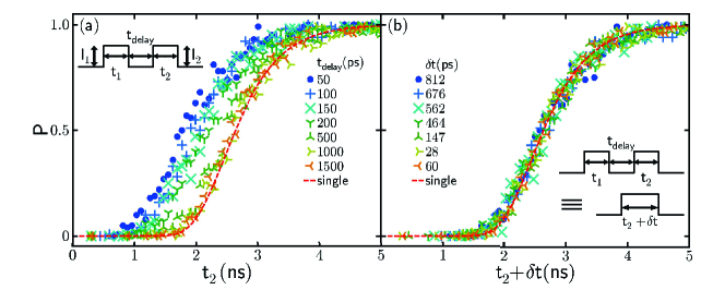
We use an arbitrary waveform generator to apply two pulses separated by a time delay , as illustrated by the inset of Fig. 1(a). The state of the spin valve is determined by a resistance measurement using a lock-in amplifier both before and after the injection of the double-current pulse. We note that the lock-in current is small enough (300 A) not to affect the spin valves and not to induce reverse switching Bedau et al. (2010b). All experiments described here were conducted at room temperature.
Initially the sample was brought into the AP state by the application of an easy-axis magnetic field of appropriate direction and magnitude. A short current pulse of positive polarity and was then applied. A longer pulse of positive polarity would eventually switch the sample into the P state (as ). However, the duration has been chosen such that the switching probability is nearly zero (), as shown by the dashed curve (i.e. the single pulse curve) in Fig. 1(a) at 0.9 ns. After a variable delay from 50 ps to 1.5 ns, a second pulse with the same amplitude () and a variable duration , from 50 ps to 5 ns, was applied. The total switching probability distribution was then measured by repeating the process to times for each pulse set.
As seen in Fig. 1(a), for delays longer than 500 ps the switching probability distribution is the same as that of the second pulse alone , which is consistent with Eq. (Time-Resolved Magnetic Relaxation of a Nanomagnet on Subnanosecond Time Scales) for . This indicates that these delays are longer than the magnetization relaxation time. The magnetization state excited by a 0.9 ns current pulse decays to equilibrium in under 500 ps, within our experimental accuracy. However, for delays less than 500 ps, the switching probability is larger than that of just a single pulse.
Remarkably, even with a composite pulse, the switching probability versus the second pulse duration is seen to follow the same functional form as that for a single pulse. This is shown in Fig. 1(b), where the probability data, shifted by an amount – a quantity that depends on the delay between the pulses – is seen to closely overlap. This clearly demonstrates that the switching probability of a composite pulse () is equal to that of a single pulse with an increased duration (). Since this is satisfied for all , a natural conclusion is that the ensemble averaged state of the sample after the first pulse and the delay () is the same as that after a single pulse with a duration of , as illustrated schematically by the pulse shapes in the inset of Fig. 1(b).
From the data shown in Fig. 1 we determine as a function of the delay . This is shown as crosses in Fig. 2. The black solid curve is an exponential fit to the data where is the lifetime of the excitation:
| (3) |
with the parameters and . For no delay, , clearly and thus , which is indeed fulfilled within the time resolution of the experiment ( ps). Eq. (3) links the duration of the excitation, the delay and the corresponding equivalent pulse duration, which is related to the magnetization relaxation rate.
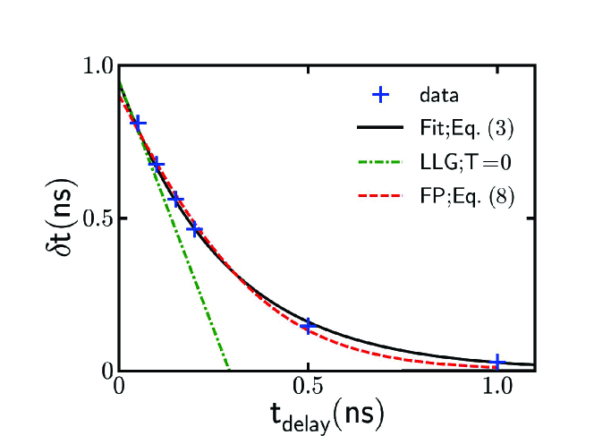
The data in Fig. 2 is unexpected at first, as a zero temperature macrospin Landau-Lifshitz-Gilbert (LLG) model predicts a linear relationship between and , as shown by the green dash-dotted line in Fig. 2. This linear relationship follows from the LLG equation. For a uniaxial nanomagnet in zero applied magnetic field, the polar angle of the magnetization , i.e. the angle between the magnetization and the easy axis, satisfies Sun (2000):
| (4) |
with:
| (5) |
| (6) |
is the relaxation time due to damping and depends on the material parameters, the anisotropy field , the Gilbert damping parameter and the gyromagnetic ratio . is typically hundreds of picoseconds. is the zero temperature critical current as we mentioned earlier, representing the threshold current for switching. It depends on the magnetization density , the nanomagnet’s volume and the spin polarization of the current . From Eq. (4) both excitation () and relaxation () follow the same functional form for small angles and are only different in their respective time constants. It is straightforward to show that the duration of a single pulse (), which brings the sample to the same state as the first pulse () followed by the delay () satisfies:
| (7) |
Hence the initial slope of versus , shown as the green dashed dotted curve in Fig. 2, depends on the current overdrive, , and provides an independent method to determine the zero temperature critical current. However, for long delays this equation is unphysical, as it predicts a negative .
A physical picture is that during the first pulse the magnetization evolves from a thermal distribution of initial angles near the north pole (, where is the energy barrier and is the thermal energy) to a larger angle . During the delay, and provided , the polar angle decays back toward the north pole. However, in this zero temperature model the magnetization decays back to , i.e. to an angle that can be less than the initial angle, .
The difference between the LLG model prediction and the experimental results can be explained by thermal fluctuations both during the excitation and relaxation processes. As is well known, thermal fluctuations lead to a spread of the initial angles of magnetization about the north pole. A spin-current pulse works to rotate the magnetization away from the easy axis direction and, in essence, amplifies these magnetization fluctuations. Once the magnetization deviates from the easy axis direction, the magnetization polar angle grows exponentially. However, thermal noise also slows down the relaxation from a simple exponential decay process predicted by the LLG equations and leads to relaxation to a thermal distribution. Therefore, thermal fluctuations not only change the timescales of the excitation and relaxation processes, they also alter their functional forms.
To model the influence of thermal fluctuations, we simulated the double pulse measurement using the Fokker-Planck Equation Brown (1963), which has the following form for a uniaxial macrospin system:
| (8) | |||||
where is the probability density of the magnetization at the angle and the time . is the dimensionless energy barrier, . For a uniaxial nanomagnet .
We start with a Boltzmann distribution centered around the easy axis in the AP state:
Where is a normalization constant so that . For the simulation we use a fixed duration for the first pulse of 0.9 ns, the same as in our experiments and vary the duration of the second pulse for different delays. By fitting the measured single pulse switching probability distribution (i.e. the red dashed curve of Fig. 1(a)) to Eq. (8). we obtain and .
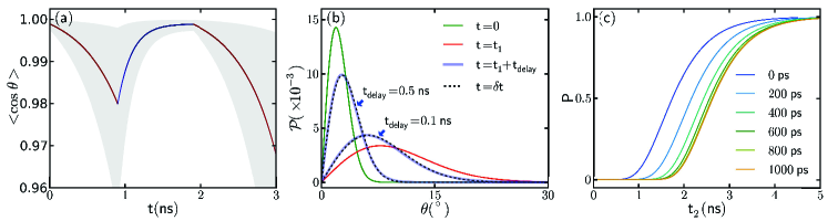
We then can track the ensemble averaged magnetization projection, as a function of time , as shown in Fig. 3(a). The shaded region depicts the angular range containing to of the states. During the first current pulse (), the switching process begins. The averaged magnetization projection decreases while the occupation probability distribution spreads out, where the majority of the distribution is still centered around . During the delay (), the averaged magnetization projection increases while the occupation probability distribution narrows toward the initial state. Then during the second pulse (), the averaged magnetization projection decreases again as the total distribution expands during the beginning part of the switching process.
We can further check whether a pulse and a delay () brings the system into the same state as a single duration pulse. Fig. 3(b) shows the occupation probability as a function of the polar angle for different delay times. The distributions for a pulse and delay (the solid light blue curves in Fig. 3(b)) overlap with those of a single pulse (dashed curves in Fig. 3(b))–which is consistent with scaling of the experimental data shown in Fig. 1(b).
The Fokker-Planck simulation results also agree quantitatively with the experimental data. As shown in Fig. 3(c) the calculated switching probability distributions have the same form independent of and can be shifted in time to coincide. The results shifts, s, are in good agreement with the experimental results, as indicated by the red dashed curve in Fig. 2. The difference between the LLG and the Fokker-Planck analysis clearly shows the influence of the thermal fluctuations, even though the total process (excitation plus relaxation) lasts less than 2 ns.
In summary, we have presented a method ideally suited to study excitation and relaxation in a magnetic nanostructure. This method only requires the generation of pulses with short durations and delays and measurement of the switching probability. It does not require resolving small signal changes at high bandwidth and it can also be used to study dynamics after a pulse, with no current applied.
Our method provides a direct (model independent) measurement of the relaxation timescale by considering when two events are correlated. We have used this method to study excitation and relaxation in a model system–a thin film nanomagnet with uniaxial anisotropy excited by spin-current pulses. We have shown that a single pulse followed by a delay leaves a nanomagnet in a state with the same ensemble average as that of a single pulse with a shorter duration . This finding is also model-independent. The s are seen to decrease exponentially, following the form of Eq. 3, and giving a relaxation time of . We note that the relaxation time is more typically obtained experimentally by fitting to an Arrhenius-Néel’s model with a variable prefactor (see, for example, Loth et al. (2012)). In general, the decay of the magnetization might be expected to be more complex than a simple exponential (Eq. 3), including multiple relaxation pathways with different timescales. However, even in such a case the directly measured relationship between and would provide information that is important for understanding such relaxation processes. Using Eq. (5) with an anisotropy field of T (see Ref. Bedau et al. (2010a)) and a gyromagnetic ratio of (Ts) (i.e. a Landé g-facto of ), we find a Gilbert damping of , a value that is larger than that determined from thin film ferromagnetic resonance measurements of the damping ( Beaujour et al. (2007)). The larger damping inferred from the data may be a consequence of the large-angle excitation of the magnetization, including non-linear effects Tiberkevich and Slavin (2007), or to changes of the magnet’s material properties associated with device nanofabrication Ozatay et al. (2008).
Interestingly, our results can be understood within a simple macrospin model that incorporates thermal fluctuations. In fitting our data to this model we obtain a dimensionless energy barrier of , which is within 25% of that expected based on the volume, magnetization and anisotropy of the nanomagnet (). Our previous results, as well as those of many other groups, have found energy barriers to reversal for long field Moritz et al. (2005); Adam et al. (2010); Thomson et al. (2006); Gopman et al. (2012) and long current pulses ( ns) Bedau et al. (2010b, a) to be only a small fraction of that expected for a macrospin, suggesting the reversal proceeds by subvolume nucleation Sun et al. (2011); Bernstein et al. (2011). For similar samples, we found that the energy barrier to reversal under long current pulses to be Bedau et al. (2010a), the macrospin value. This suggests that the reversal modes in the short-time nonequilibrium limit are distinct from those in the long-time limit, as the system may not have time to follow minimum energy paths or be driven from these paths by the spin transfer torque. The fundamental explanation is an open question. We expect that the dependency of the effective energy barrier on pulse amplitude can be further studied by our method with different pulse conditions. Our double pulse method, which provides access to the intrinsic time scales of the excitation and relaxation dynamics, can be used in other cases where the readout signal is also small, such as current induced domain wall motion.
Acknowledgments
This research was supported at NYU by NSF Grant DMR-1006575, USARO Grant No. W911NF0710643 as well as the Partner University Fund (PUF) of the Embassy of France.
References
- Koch et al. (2004) R. H. Koch, J. A. Katine, and J. Z. Sun, Physical Review Letters 92, 088302 (2004).
- Garzon et al. (2008) S. Garzon, L. Ye, R. A. Webb, T. M. Crawford, M. Covington, and S. Kaka, Phys. Rev. B 78, 180401 (2008).
- Schumacher et al. (2003) H. W. Schumacher, C. Chappert, P. Crozat, R. C. Sousa, P. P. Freitas, J. Miltat, J. Fassbender, and B. Hillebrands, Phys. Rev. Lett. 90, 017201 (2003).
- Vaterlaus et al. (1991) A. Vaterlaus, T. Beutler, and F. Meier, Phys. Rev. Lett. 67, 3314 (1991).
- Beaurepaire et al. (1996) E. Beaurepaire, J.-C. Merle, A. Daunois, and J.-Y. Bigot, Phys. Rev. Lett. 76, 4250 (1996).
- Devolder et al. (2008) T. Devolder, J. Hayakawa, K. Ito, H. Takahashi, S. Ikeda, P. Crozat, N. Zerounian, J. V. Kim, C. Chappert, and H. Ohno, Physical Review Letters 100, 057206 (2008).
- Cui et al. (2010) Y. T. Cui, G. Finocchio, C. Wang, J. A. Katine, R. A. Buhrman, and D. C. Ralph, Physical Review Letters 104, 097201 (2010).
- Eq (2) We note the Eq. (2) applies to cases in which both pulses are of the same polarity and both increase the probability of switching from the initial state to the final state . This applies to our system as shown in Fig. 1. Eq. (2) would need to be modified for pulses of opposite polarity and well as for nanopillars with more complex magnetic anisotropies, such as those studied in Ref. Garzon et al. (2008).
- Bedau et al. (2010a) D. Bedau, H. Liu, J. Bouzaglou, A. D. Kent, J. Z. Sun, J. A. Katine, E. E. Fullerton, and S. Mangin, Applied Physics Letters 96, 022514 (2010a).
- Bedau et al. (2010b) D. Bedau, H. Liu, J. Z. Sun, J. A. Katine, E. E. Fullerton, S. Mangin, and A. D. Kent, Applied Physics Letters 97, 262502 (2010b).
- Mangin et al. (2006) S. Mangin, D. Ravelosona, J. A. Katine, M. J. Carey, B. D. Terris, and E. E. Fullerton, Nat Mater 5, 210 (2006).
- Mangin et al. (2009) S. Mangin, Y. Henry, D. Ravelosona, J. A. Katine, and E. E. Fullerton, Appl. Phys. Lett. 94, 012502 (2009).
- Min et al. (2009) T. Min, J. Z. Sun, R. Beach, D. Tang, and P. Wang, Journ. of Appl. Phys. 105, 07D126 (2009).
- Sun (2000) J. Z. Sun, Phys. Rev. B 62, 570 (2000).
- Brown (1963) W. F. Brown, Phys. Rev. B 130, 1677 (1963).
- Loth et al. (2012) S. Loth, S. Baumann, C. P. Lutz, D. M. Eigler, and A. J. Heinrich, Science 335, 196 (2012).
- Beaujour et al. (2007) J.-M. L. Beaujour, W. Chen, K. Krycka, C.-C. Kao, J. Z. Sun, and A. D. Kent, Eur. Phys. J. B 59, 475 (2007).
- Tiberkevich and Slavin (2007) V. Tiberkevich and A. Slavin, Phys. Rev. B 75, 014440 (2007).
- Ozatay et al. (2008) O. Ozatay, P. G. Gowtham, K. W. Tan, J. C. Read, K. A. Mkhoyan, M. G. Thomas, G. D. F. P. M. Braganca, E. M. Ryan, K. V. Thadani, J. Silcox, et al., Nature Materials 7, 567 (2008).
- Moritz et al. (2005) J. Moritz, B. Dieny, J. P. Nozieres, R. J. M. van de Veerdonk, T. M. Crawford, D. Weller, and S. Landis, Applied Physics Letters 86, 063512 (2005).
- Gopman et al. (2012) D. B. Gopman, D. Bedau, S. Mangin, C. H. Lambert, E. E. Fullerton, J. A. Katine, and A. D. Kent, Applied Physics Letters 100, 062404 (2012).
- Adam et al. (2010) J.-P. Adam, J.-P. Jamet, J. Ferre, A. Mougin, S. Rohart, R. Weil, E. Bourhis, and J. Gierak, Nanotechnology 21, 445302 (2010).
- Thomson et al. (2006) T. Thomson, G. Hu, and B. D. Terris, Physical Review Letters 96, 257204 (2006).
- Sun et al. (2011) J. Z. Sun, R. P. Robertazzi, J. Nowak, P. L. Trouilloud, G. Hu, D. W. Abraham, M. C. Gaidis, S. L. Brown, E. J. O’Sullivan, W. J. Gallagher, et al., Phys. Rev. B 84, 064413 (2011).
- Bernstein et al. (2011) D. P. Bernstein, B. Brauer, R. Kukreja, J. Stohr, T. Hauet, J. Cucchiara, S. Mangin, J. A. Katine, T. Tyliszczak, K. W. Chou, et al., Phys. Rev. B 83, 180410 (2011).