Impact of wettability correlations on multiphase flow through porous media

In the last decades, significant progress has been made in understanding the multiphase displacement through porous media with homogeneous wettability and its relation to the pore geometry. However, the role of wettability at the scale of the pore remains still little understood. In the present study the displacement of immiscible fluids through a two-dimensional porous medium is simulated by means of a mesoscopic particle approach. The substrate is described as an assembly of non-overlapping circular disks whose preferential wettability is distributed according to prescribed spatial correlations, from pore scale up to domains at system size. We analyze how this well-defined heterogeneous wettability affects the flow and try to establish a relationship among wettability-correlations and large-scale properties of the multiphase flow.

Keywords: Multiphase fluid flows; Mesoscale simulations; Multi-Particle Collision dynamics; Wettability.

 

Introduction

The displacement of immiscible fluids through porous media is subject of scientific interest, as it is involved in many industrial and technological applications, such as oil recovery, water flows, and soil treatment. Understanding the dynamics of this process at the pore scale is crucial but, on the other hand, very challenging due to the many involved parameters, from the competition between viscous and capillary forces to the wetting properties and porous structure of the substrate.

In the last decades visualization experiments using simplified micromodels of porous media have provided a detailed description of immiscible flow [1, 2, 3, 4, 5]. A number of dynamical regimes are distinguished in terms of capillary number (ratio of viscous to capillary forces), viscosity ratio (ratio of the viscosity of the injected fluid to the viscosity of displaced fluid), and wetting conditions.

In the limit of high injection rates, the front advance critically depends on the viscosity ratio of the fluids. When the injected fluid has a lower viscosity than the displaced fluid, the situation is highly unstable and ramified viscous fingers are observed. In the opposite case, when the injected liquid has a higher viscosity, the front exhibits a stable displacement with a steady width. However, in the limit of very slow injection rates the displacement depends entirely on the capillary forces. In this limit, the pressure drop due to the viscous flow field can be neglected and the front roughens due to capillary pressure fluctuations at the pore level. This capillary fingering regime has been successfully described by means of statistical models as invasion-percolation [6, 7, 8] and some more sophisticated pore-network models [9, 10, 11].

On the other hand, the development of analytical and computational techniques for fluid dynamic simulations have provided a great advance in the numerical approach to this phenomenon  [12, 13, 14, 15]. However, the continuous description is not sufficient to understand the multiphase flow at the pore scale due to the wide range of scales involved in this process. To do so, one has to comprehend the interfacial dynamics - especially the fluctuations generated at the contact line by the substrate heterogeneities- and, from this microscopical information, build up a coherent macroscopic description of the flow.

Mesoscopic simulation techniques provide a robust numerical approach with high enough computational efficiency at the scale of interest. The fundamental idea is to design simplified kinetic models that coarse-grain the essential microscopical physics into a mesoscopic description, so that the averaged properties obey the macroscopic transport equations, in particular Navier-Stokes and mass diffusion equations. These mesoscale algorithms properly reproduce the complex behavior of systems like colloidal suspensions or microemulsions, and have the major advantage of dealing with changing interfacial topologies in a natural way. The most extended ones are direct Monte-Carlo simulations (MC) [16], Lattice Boltzmann Method (LBM) [17], Dissipative-Particle Dynamics (DPD) [18] and Multi-Particle Collision models (MPC) [19, 20].

In the present paper we employ the MPC method, originally proposed by Malevantes and Kapral [19], to simulate the displacement of immiscible fluids in a two-dimensional porous medium at low capillary numbers. This particle mesoscopic approach is an alternative simulation technique that, compared with the most extended LBM, directly includes thermal fluctuations, allows to treat systems with an arbitrary number of phases, and provides detailed information about the dynamics at the fluid boundaries on any scale, as the definition of the physical system is independent on the coarsening process of the mesoscopic approach.

To deal with multiple phases we adopt the MPC multicolor generalization proposed by Inoue et al. [21]. We incorporate to the model the definition of relative adhesion of the fluid phases to the solid phase, in order to control the wetting conditions. Our aim is to provide a numerical tool to study the influence of wettability on immiscible multiphase flow at the pore scale. Although significant progress has been made toward understanding the effect of homogeneous substrate wettability, the role of heterogeneous wettability remains still little understood due to the difficulty of controlling its spatial definition at the scale of the pores [22, 23, 24, 25]. Here, we prepare different spatial correlations of local wettability in our numerical simulations and analyze how they influence the dynamics, trying to establish a relationship with large-scale properties of the multiphase flow.

In the next Section 2, we provide a description of the MPC method including the wettability implementation. In Section 3 we analyze the relevant parameters interfacial tension and viscosity, and their consistency with thermal fluctuations in terms of capillary waves. In Section 4 we present our results on multiphase flow through porous media analyzing the role of wettability for both homogeneous and heterogeneous cases.

MPC model

The fluid is modeled by a large number $N$ of point-like particles, each with the same mass $m$ which move with a continuous distribution of velocities. The dynamics of the particles consists in a sequence of streaming and collision steps. In the streaming step, the particles move deterministically during a time interval $\Delta t$ according to their individual velocity $v_{i}(t)$.

In order to introduce an interaction among particles, i.e. an exchange of linear momentum, they are sorted into collision cells $\xi$. As we are working in two spatial dimensions, we use a regular square grid of typical size $a$ where the number of particles per cell, $N_{\xi}$, fluctuates around an average value $N_{c}$. In every collision step, the velocities of the particles are decomposed into the center of mass velocity $\vec{u}_{\xi}$ of the particles in a cell and a remaining, fluctuational part. An effective exchange of linear momentum between the particles in cell is achieved through a rotation of the fluctuational velocity components in each cell. The velocity after the effective collision step at time $t+\Delta t$ is:

$$\vec{v}_{i}(t+\Delta t)=\vec{u}_{\xi}(t)+\Omega[\vec{v}_{i}(t)-\vec{u}_{\xi}(t)].$$ (1)

As we assume molecular chaos, the rotation operator $\Omega$ in eqn. (1) must be statistically independent in each cell and in each time-step. Galilean invariance is guaranteed by shifting the coarse-graining grid randomly before each collision step [26]. As linear momentum and mass is conserved, the spatially averaged particle motion displays hydrodynamic behavior on large length scales. Furthermore it has been shown that there is an H-theorem for this algorithm [19].

To deal with multiple immiscible fluid phases we adopt a variant of the MPC algorithm proposed by Inoue et al. [21], that induces phase segregation. This method has been already successfully applied to study the distribution of droplets in bifurcating micro-channels [27]. In this algorithm, each phase is assigned a label (color) $c=1,...,N_{ph}$. At each time step and cell $\xi$ the color flux

$$\vec{q}_{c}(\xi)=\sum_{i=1}^{N_{\xi}}(\vec{v}_{i}-\vec{u}_{\xi})\cdot\delta_{c,c_{i}}\ ,$$ (2)

and the color-gradient field

$$\vec{F}_{c}(\xi)=\sum_{j=1}^{N_{ph}}\kappa_{cj}\cdot\vec{\nabla}\,n_{j}$$ (3)

are calculated, where $\vec{\nabla}\,n_{j}$ is the local gradient of the number density $n$ of particles with color $j$ which is estimated from the number of particles of the same color in the next-nearest neighbor cells. The matrix $\kappa_{ij}$ is the interaction matrix that defines the cohesion/adhesion between fluid phases of color $i$ and $j$. Then the multicolor potential energy is defined as

$$U(\xi)=\sum_{c=1}^{N_{ph}}U_{c}(\xi)=\sum_{c}-\vec{q}_{c}(\xi)\cdot\vec{F}_{c}(\xi)$$ (4)

and the operator $\Omega$ is chosen such to minimize $U(\xi)$ (in the case of 2-dimensions this simply means $\Omega(\theta_{\xi})$ with $\partial U/\partial\theta_{\xi}=0$, where $\theta_{\xi}$ is the angle of rotation respect the center of the cell). Let us mention here that this segregation algorithm generates a depletion layer at the fluid-fluid interface that effectively reduces the transport of shear stress through the fluid interface and, in particular, a finite slip between the two fluid phases. However, as we are mainly working in the regime of small capillary numbers, where normal stresses dominate the dynamics at the fluid interfaces, this effect is not relevant. For a more detailed description of the model, the reader is referred to [21].

Thermostatting is required in any non-equilibrium MPC simulation due to viscous heating. Here we apply a simple local profile-unbiased thermostat that ensures control of the thermal fluctuations in the bulk as well as on the solid walls while keeping unaffected the velocity field [28]. The relative velocities to the center-of-mass velocity of each cell $\xi$ are rescaled after each collision step as $\vec{v_{i}}=\lambda(\xi)\cdot\vec{v_{i}}$, where $\lambda(\xi)=k_{B}TN_{\xi}d/\sum_{i=1}^{N_{\xi}}m\cdot(\vec{v_{i}}-\vec{u_{\xi}})^{2}$ with $d$ dimensions.

Wettability implementation

The multicolor model was originally proposed without specifying any wetting condition [21]. However, wettability plays a pivotal role in immiscible flow through porous media and, hence, needs to be thoroughly implemented in the algorithm. To this end we developed a method that accounts for relative adhesion of two fluids to the solid surface while, at the same time fulfilling the proper fluid dynamic boundary conditions.

First, let us review the treatment of the fluid dynamic boundary conditions for MPC algorithms. In order to guaranty non-slip boundary condition for the average fluid velocities, we employ the generalization of the bounce-back rule for partially filled cells [29]. In the naïve formulation of the bounce back rule, particles travel back into the direction of their incidence after having collided with the solid boundaries. However, because the position of the solid boundaries relative to the coarse-graining grid changes between every interparticle collision step, it is necessary to add a virtual phase resting in the walls. This virtual phase takes part in the collision procedure to match the bulk particle density in the underfilled cells. These wall-particles are generated before and removed after every interparticle collision step, and guarantee a no-slip boundary condition at the walls [29].

To define the wetting conditions we include the virtual wall-phase in the definition of the interaction matrix, adding an extra term that determines the wall interaction for each of the fluid phases present in the system. By tuning the relative strength of each of them, we can achieve different contact angles of the fluid interface at the solid walls. In the following we will refer to a system of two phases, namely fluid (1) and fluid (2), in contact with the wall (3), and our matrix is $\kappa_{ij},i,j=1,2,3$.

In order to reduce the slip generated by the phase segregation procedure, we set $\kappa_{13}=1$ that fixes the surface tension $\sigma_{13}=0$. As there is no distinction between phase (1) and (3) there will be no slip for fluid phase (1) at the wall (3). Then, our interaction matrix will have the form

$$\kappa=\left(\begin{array}[]{rrr}1&-1&1\\ -1&1&\kappa_{23}\\ 1&\kappa_{23}&1\end{array}\right)$$ (5)

According to the definition of the Young’s contact angle, referred to a droplet of fluid (2) resting on the wall and immersed in the ambient fluid (1), we have $\sigma_{12}\cos\theta+\sigma_{23}=\sigma_{13}$ that is simplified to $\sigma_{12}\cos\theta+\sigma_{23}=0$ with the condition $\kappa_{13}=1$. In the remainder of this article we will focus on three particular cases: i) For $\kappa_{23}=-1$ we find $\sigma_{23}=\sigma_{12}$ and therefore a contact angle of $\theta=180^{\circ}$ while ii) $\kappa_{23}=1$ leads to $\sigma_{23}=0$ and a contact angle of $\theta=90^{\circ}$. iii) In the limit $\kappa_{23}\gg 1$ we have $\sigma_{23}<0$ and therefore $\theta\rightarrow 0^{\circ}$.

In the following, as we denote the invading phase by (2), we will refer to these cases as non-wetting ($\kappa_{23}=-1$), neutral wettability ($\kappa_{23}=1$) and total wetting, for which we consider $\kappa_{23}=2$. The introduction of a negative surface tension for the wetting case allows us to avoid the formation of a depletion layer originated by the phase segregation mechanism and avoid any slippage of the invading phase (2) at the wall. In Fig. 1 we show the equilibrium configurations of a droplet of phase (2) between two solid parallel walls for the three wetting conditions we consider.

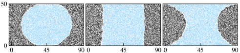
Figure 1: Equilibrium contact angle for the three considered wetting conditions in a planar geometry (from left to right): non-wetting, neutral wettability and total wetting.

System parameters and thermal fluctuations

In this section we analyze how macroscopic quantities, like the dynamic shear viscosity and interfacial tension, emerge from the definition of our microscopic system parameters, that are the cell size $a$, time step $\Delta t$, particle mass $m$, mean number density $N_{c}$ defined as the average number of particles per cell, temperature $temp$ (in $k_{B}T$ units), and the entries $\kappa_{ij}$ of the interaction matrix. We normalize $\Delta t=1$, $a=1$, $m=1$, and set $N_{c}=10$. For all the simulations we fix $temp=10^{-3}$, which implies a mean free path for a particle in between two consecutive collisions $\lambda=\Delta t\sqrt{temp/m}\approxeq 0.03$.

The behavior of a single phase does not depend on the strength of the self-interactions among particles of the same species, so we can normalize the diagonal terms of the interaction matrix to $\kappa_{ii}=1$ without loss of generality. Fitting the velocity profile of a simple fluid in a planar channel to the Poiseuille flow we estimate the value of the dynamic viscosity of the fluid phase to be $\mu=0.750\,m/a\Delta t$ for the set of parameters considered.

Since the interfacial tension the fluid phases (1) and (2) is not a direct input for our algorithm but is controlled by the interaction term $\kappa_{12}$, we estimate it by terms of the Laplace law. Initially a square droplet of fluid (1) is placed in the center of a simulation box filled with fluid (2). After a transient time, it relaxes to a configuration fluctuating around a circular shape. We measure the radius $R$ of the averaged droplet contour and the corresponding difference $\Delta P=P_{1}-P_{2}$ between the pressure in the droplet (1) and the in the ambient fluid (2) for different values of the interaction term $\kappa_{12}$. The pressure is computed by means of the microscopic definition of the local stress tensor

$$T_{\alpha\beta}=-\frac{1}{V}\sum_{i=1}^{N_{c}}m_{i}\cdot v_{i\alpha}\cdot v_{i\beta}-\frac{1}{V\Delta t}\sum_{i=1}^{N_{c}}\Delta p_{i\alpha}\cdot r_{i\beta}~{},$$ (6)

where $\vec{v}_{i}$ is the velocity of the particle before the collision step, $\Delta\vec{p}/m_{i}=\vec{v}_{i}(t+\Delta t)-\vec{v}_{i}(t)$ and $\vec{r}_{i}$ is the particle position referred to the center of the cell. The expression eqn. (6) for the stress tensor is given, e.g., in Ref. [30].

Plotting $\Delta P$ against the radius of the averaged droplet contour in Fig. 2 shows the expected linear relation $\Delta P\propto 1/R$ according to Laplace’s law. The proportionality constant is the value of the interfacial tension $\sigma$. We observe that the interfacial tension becomes non-zero as soon as $\kappa_{12}\neq\kappa_{11}=\kappa_{22}$. After a short rise while decreasing $\kappa_{12}$ , it describes a plateau for values $\kappa_{12}\lesssim-1$. According to this, in forthcoming simulations we fix our fluid-fluid interaction $\kappa_{12}=-1$, for which we have an interfacial tension $\sigma=(0.0011\pm 0.0004)\,m/\Delta t$.

Finally, we check that the thermal fluctuations are consistent with the estimated value of the interfacial tension analyzing the capillary waves observed on a planar fluid-fluid interface. An initially straight interface will roughen by the motion of thermally activated capillary waves. In the capillary wave spectrum, each Fourier component $h_{k}=\sum_{j=0}^{L-1}h_{j}(t)e^{2\pi ijk/L}$ of the interface displacement contributes according to the equipartition theorem

$$\langle\lvert h_{k}\lvert^{2}\rangle=\frac{K_{B}TL}{\sigma k^{2}}$$ (7)

leading to an interface roughness proportional to $\sqrt{k_{B}T/\sigma}$ [31, 32]. In Fig. 2 we plot the average amplitudes $\langle\lvert h_{k}\lvert^{2}\rangle$ of the planar capillary waves as function of the wave number $k$. As expected from the assumption of a wave number independent of the interfacial tension $\sigma$ we observe that the spectra for different system sizes collapse for the value $\sigma=(0.0023\pm 0.0008)m/\Delta t$, which is in good agreement with the estimate obtained from the Laplace law for circular droplets of different radii. Therefore, the model displays the correct thermodynamic behavior and interfacial fluctuations.

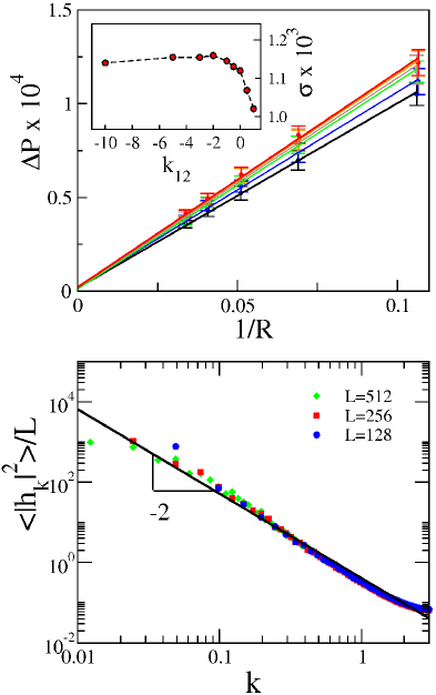
Figure 2: Interfacial tension analysis. Top: Laplace $\Delta P=P_{1}-P_{2}$ plotted vs. the interfacial curvature $1/R$ for droplets of different size. In the inset we plot the interfacial tension $\sigma$ estimated from the slope of the pressure/curvature plot vs. $\kappa_{12}$. Bottom: Power spectrum of thermally excited capillary wave amplitude for a planar interface. The spectra for different system sizes collapse according to eqn. (7) for $\sigma=(0.0023\pm 0.0008)\,m/\Delta t$, in agreement with the estimate from the Laplace pressure.

Flow in porous media

Immiscible displacements in porous media with both capillary and viscous effects can be characterized by two dimensionless numbers, the ratio ${\rm M}=\mu_{\rm i}/\mu_{\rm d}$ of the dynamic viscosities $\mu$ of the invading fluid (i) and the displaced fluid (d), and the imposed capillary number, i.e., the ratio of viscous to capillary forces given by ${\rm Ca}=\sigma\,v/\mu_{\rm i}$, where $\sigma$ is the interfacial tension of the fluid interface and $v$ is the average front velocity.

When viscous forces dominate (${\rm Ca}>1$), the invading front exhibits either stable advance or viscous fingering (${\rm M}>1$ and ${\rm M}<1$ respectively). However, at low ${\rm Ca}$ the displacement is solely governed by capillary forces [1, 2, 3, 4, 5]. This propagation mechanism can be captured using concepts from invasion-percolation [6, 7, 8, 9, 10, 11]. In the following, we consider a porous matrix which is completely filled with the initial fluid phase (d). By means of an applied pressure gradient a secondary fluid phase (i) is pushed into the matrix displacing phase (d).

System setup

The porous matrix is represented by an assembly of non-overlapping circular disks with fixed position whose preferential wettability by the invading fluid (i) can be selected from the three different cases: non-wetting, neutral and wetting. Our porous region is a two-dimensional rectangular channel with length $L$ and width $H$ that extents $0<x<L$ in the direction of the applied pressure gradient. Periodic boundary conditions are considered into orthogonal direction.

To generate the pressure gradient that drives the flow we define an inflow region $x\in[-I,0]$ being free of obstacles where a constant body force $g$ acts into the x direction on the particles. The extension of this inflow region is $I\approx 0.3L$ into the direction of the flow. As a result of the body force in the inflow region a pressure gradient builds up that drives the fluid particles through the obstacles.

The value of $g$ is constrained to be small enough in order to avoid compression of the fluids, i.e. a Mach number ${\rm Ma}=v/c<1$, where $c$ is the speed of sound. In the following we will apply $g=O(10^{-5})$, which gives us ${\rm Ma}=O(10^{-2})$, Reynolds numbers ${\rm Re}=\rho v\mathcal{L}/\mu=O(10^{-1})$ with $\mathcal{L}$ the typical distance between the obstacles and mass density $\rho$, and ${\rm Ca}=O(10^{-1})$ for the system sizes and the set of parameters we consider, as introduced in section 3.

Homogeneous wettability

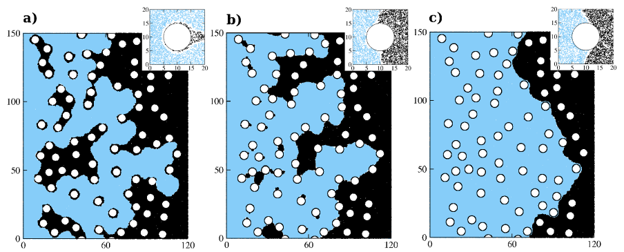
Figure 3: Snapshots of the invading front for the three cases of homogeneous wettability: a) non-wetting, b) neutral wettability and c) wetting. The inset of each panel shows a detail of the dynamics around one single obstacle. The different advancing mode of the front can be appreciated.

First we analyze the dynamics of the forced displacement in a substrate composed of monodisperse disks. Previous experiments in quasi-2d micromodels [7, 5], as well as numerical approaches [9, 33] clearly indicate that wetting conditions strongly influence the displacement of immiscible fluids through porous media in the capillary fingering regime.

These analyses also evidence that, when viscous forces are not strictly zero, the flow may be influenced by the pore geometry. For instance, in the case of a broad throat-size distribution the viscous pressure drop may become on the order of magnitude of the difference of Laplace pressure between a small and a large throat, what makes the invasion-percolation description not longer valid [8, 5, 12].

To discern the effect of wettability from effects related to pore geometry and from dynamic front instabilities (i.e., the Saffman-Taylor instability) we strictly consider equal dynamic viscosities ${\rm M}=1$ and porous matrices with low packing density $\phi=A_{o}/A$, where $A_{o}$ is the area occupied by the obstacles an $A$ is the total area of the simulation box. In the following we employ a random configuration of circular obstacles with radius $r$, generated by means of random sequential addition [34], for which we impose $\phi=0.15$ and a minimal separation distance $d=2r$ between the obstacles.

Figure 3 displays snapshots of the invading front for the three different cases of wettability, as well as details of the flow around one single obstacle for each case. Initially the matrix is completely filled with phase (d) and then the invading fluid (i) is driven from the left by means of the pressure gradient generated in the inflow region. The applied body force on particles within this region is $g=1.0\times 10^{-5}$, what generates a pressure gradient $\Delta P\approx 0.008\,m/\Delta t^{2}$. In these figures we show snapshots of the invading front close to percolation. They correspond to different simulation times as the velocity of invasion clearly depends on the wettability.

In the non-wetting case we observe that, almost from the very beginning, the front roughens and fingers are formed. The fluid in these fingers pinches off leaving behind a number of disconnected domains of the displaced fluid which are trapped between the disks. This gives rise to a considerably high residual saturation as we observe in Fig. 4, where the evolution of saturation $S=A/A_{0}$ is depicted versus time, with the area $A$ of displaced phase (d) and total area $A_{0}$ of the void space. On the other hand, the formation of new fluid-fluid interface slows down the dynamics, as we observe when plotting the flux measured at the end of the porous matrix for both fluid phases. The flux of the invading fluid, instead of remaining constant in time, as would correspond to a stable front, clearly decreases in time as the invading fluid describes intricate paths through the porous structure. These plots also shows that even after breakthrough, when the flux of the displaced fluid displays a first peak, some other fingers still develop, and we observe a secondary percolation of the invading fluid before reaching the steady state at which the flux becomes constant.

In the case of neutral wettability the dynamics of the invading front is considerably different. We observe much smaller trapped clusters of the displaced fluid. A similar behavior has been reported in Ref [5] for quasi-2d experiments. This is clearly manifested by the lower value of residual saturation in Fig. 4. However, in this graph we observe that the velocity of invasion, that we define as the velocity of an equivalent stable front with $v\approx LdS/dt$ for the same imposed ${\rm Ca}$, is very similar for both the non-wetting and the neutral case until the curves saturate. As in both situations the work injected into the system can be invested either in viscous dissipation or in formation of new fluid-fluid interfaces, this means that the length of the fluid-fluid interface should be also comparable in both cases during this time span. To figure this out and complement this analysis, we depict in Fig. 5 how the length of the fluid-fluid interface evolves in time. Certainly, we observe that the length growth of the fluid-fluid interface is very similarly for both cases during this time span, after which it practically remains constant for the non-wetting case while is drastically reduced, practically constant, for the neutral case.

Finally, we consider the case of perfectly wetting obstacles for the same imposed pressure gradient as in the previous cases. In this case the front advance is clearly stable, and the flux of the invading phase fluctuates around a constant value as well as the length of the fluid-fluid interface remains constant until breakthrough. In this case the time until percolation is much shorter, which is readily explained by the gain in wetting energy in addition to the pressure gradient. After percolation, virtually all the initial saturation is taken out as can be seen in Fig. 4.

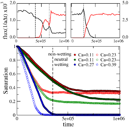
Figure 4: Saturation of the displaced phase vs. time for homogeneous wettability: non-wetting (red), neutral (green) and wetting (blue). Results are shown for low driving $g=1.0\times 10^{-5}$ (full symbols) and higher driving $g=1.5\times 10^{-5}$ (open symbols). The capillary number for each case is specified in the inset. Dashed line is depicted for comparison with Fig. 5. Top: Evolution of the flux of the invading (black) and displaced fluid phase (red) during the invasion for the case of non-wetting (left) and wetting (right) pore walls for the low driving case. The dashed and dotted lines indicate breakthrough and secondary percolation, respectively.

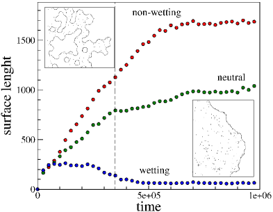
Figure 5: Evolution of the fluid-fluid interfacial length in time for the three different homogeneous wetting conditions considered: non-wetting, neutral and wetting from top to bottom. In the insets we show a detail of the fluid-fluid interface for the non-wetting (top) and wetting (bottom) cases, corresponding to the snapshots presented in Fig 3. Dashed line is depicted for comparison with Fig. 4.

Next we analyze how the front advance depends on the applied driving $g$. In accordance with experimental results [8] we observe shorter percolation times and lower values of the residual saturation for higher driving $g=1.5\times 10^{-5}$. For comparison with the previous results at lower $\rm Ca$, we include the evolution of $S$ vs. time in Fig. 4. It is clear that, in the case of higher Ca, the capillary fingers can overcome more easily the local Laplace pressure required to invade the pores, that in this regime is basically given by the pore geometry (at least in the limit ${\rm M}=1$). This clearly favors the extraction of initial fluid, as we can appreciate in Fig. 4, where the residual values are smaller than the ones obtained for any case of wettability at smaller ${\rm Ca}$.

Heterogeneous wettability

In this section we analyze how wettability heterogeneities at pore scale affect the dynamics of fluid invasion. Previous works dealing with heterogeneous wetting conditions are present in the Literature, for instance experiments dealing with a mixture of wetting and non-wetting beads [35] or composite porous medium made of blocks of the same permeability but opposite wettability [25]. We find also detailed numerical approaches, like simulations of immiscible displacement through a realistic pore structure whose wettability distribution is taken from microtomographic images of reservoir rocks [24].

However, our aim here is to analyze the effect of such heterogeneities using well-characterized spatial distribution of wettability down to the pore scale. This implies being able to independently assign to each pore a well defined wettability according to a predefined spatial distribution.

In order to identify the pores in our porous matrices we consider a Delaunay triangulation based on the centers of the obstacles. According to the construction no obstacle-center is inside the circumcircle of any other triangular pore. Once defined the pores, we independently assign wetting conditions to each of them. This means that our obstacles are divided in sectors according to the pore definition, and different wettabilities are assigned to each of them, to build up an heterogeneous pattern at the pore scale.

Figure 6 shows the distribution of two immiscible fluids of an initially random mixture in presence of a pore-scale wettability pattern after spontaneous phase separation. It can be observed that each of the two immiscible fluids is in contact solely to the highly wettable parts of the pore wall. Deviations from an ideal distribution can be easily explained by the presence of thermal fluctuations.

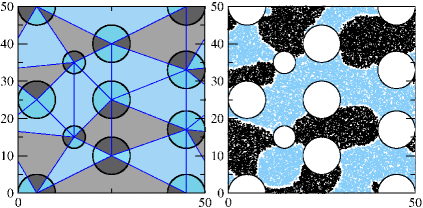
Figure 6: Pores defined in terms of Delaunay triangularization and wettability definition at pore scale. On the right we show the final state of a 1:1 binary mixture of two immiscible fluids after relaxation, which matches with the imposed wettability pattern defined in terms of wetting and non-wetting pores.

Next we consider the same porous geometry than that of section 4.2 and impose wetting patterns with well defined spatial correlations, in terms of wetting and non-wetting domains with typical size $\xi$. To generate these patterns we start from a randomly distributed wettability for each pore and introduce correlations by means of a simple stochastic procedure in which

• we randomly choose a pair of pores

• we assign to the second pore the wettability of the first one with probability $p(\ell)$ that depends on the distance $\ell$ between both of them, i.e., the distance between the incenters of the triangles.

We choose this function to be the error function $p(\ell)=\frac{1}{2}\left(1+erf\left(\frac{\mu-\ell}{\sigma\sqrt{2}}\right)\right)$, that exhibits a sharp transition between $1$ and $0$ at a typical distance $\mu$. We fix $\sigma=3\mu$. Due to computational system-size limitations, the number of pores in our system is not large enough and there is some deviation between the typical distance $\mu$ imposed in the pattern generation and the spatial correlation length $\xi$ that the patterns finally exhibit. However, when fitting the spatial correlation of the samples to the functional form $C(\ell)\backsim exp(-\ell/\xi)$ we obtain a correlation length $\xi$ that depends linearly on the $\mu$ parameter as $\xi=1.2+\mu$ (goodness of fit $C=0.98$). On the other hand, the ratio the total area occupied by the wetting and non-wetting pores, $A_{w}$ and $A_{nw}$ respectively, is approximately constant for all the patterns $A_{w}/A_{n-w}\approx 0.5$.

In the following we will analyze how the variation of the spatial correlation of our wettability patterns affect the invasion when considering the same arrangement of obstacles than that of the homogeneous case.

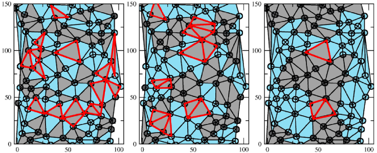
Figure 8: Pore invasion for the same single realizations presented in Fig. 7 with spatial correlations of pores wettability corresponding to $\mu=4,6,12$ (from left to right). The invaded non-wetting pores are marked in red. The invasion process is clearly dominated by the geometrical disposition of the wetting patterns. At low correlation the front invades many small non-wetting domains, and the size of these invaded non-wetting domains increases with the correlation length. However, for high enough correlations only few single bottle-neck non-wetting pores are invaded, and the front rapidly percolates.

In the case of spatially uncorrelated wettability, i.e. small values of $\mu$, the front needs to invade many small non-wetting domains in order to percolate. We show these pore-breakthrough events in Fig. 8 for a given realization at small domain size with $\mu=4$. For the sake of better visibility the invaded non-wetting pores are marked in red.

If we increase the correlations, percolation of the invading fluid requires filling of larger non-wetting domains. This slows down the invading process as can be seen in Fig. 7, where we show the evolution of saturation $S$ for different values of the $\mu$ parameter. On the other hand, invading these larger non-wetting domains is more expensive in terms of surface energy, and therefore many of the non-wetting domains remain unexplored. As we see from the plots shown in Fig. 7, the residual saturation increases monotonously with the correlation length for this range of intermediate correlations.

Finally, for even larger correlation lengths we observe that only few bottle-neck non-wetting pores need to be invaded to achieve percolation and the invading fluid rapidly floods the large wetting domains. Now, the residual saturation is virtually given by the ratio $A_{w}/A_{n-w}$ and does not depend any more on the correlation length.

We have to mention here that these results are statistically poor due to the computational limitations to go for larger systems and have better defined spatial correlations. However, they are still good enough to show qualitatively that the fluid invasion is sensitive to the spatial distribution of wettability at pore scale. In Fig. 7 we show the dependence of the residual saturation after the invasion on the correlation parameter $\mu$, where each value has been averaged over several equivalent samples and independent realizations on each of them. The increase of the residual saturation with the correlations of the wettability patterns is clearly appreciable, as well as the subsequent plateau due to the presence of bottle-neck non-wetting pores.

Finally, we conclude this analysis increasing the imposed ${\rm Ca}$, as we did in the case of homogeneous wettability. Now the higher pressure gradient washes out the effect of the wettability patterns on the flow advance. We appreciate in Fig. 7 that the saturation curves for different $\mu$ are similar and the difference in residual saturation diminishes, in comparison with the lower driving case.

Conclusions

We have adapted the MPC multicolor algorithm to control the wetting conditions at the solid boundaries in order to simulate immiscible displacement trough porous media. This is an alternative particle-based simulation approach that provides microscopical details of the dynamics at the fluid boundaries and directly incorporates thermal fluctuations.

As a first application of this method, we analyze the dependence of the multiphase dynamics on the spatial correlations of wettability, analyzing the evolution of the initial saturation and particle flux for different wetting conditions.

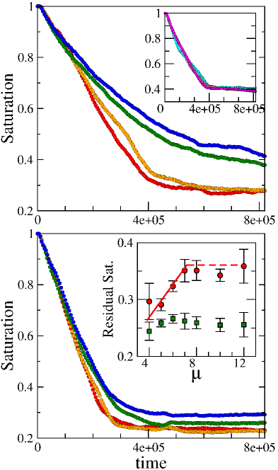
Figure 7: Saturation as function of time for heterogeneous wettability patterns with different $\mu$ (single realization for each case). Top: At intermediate correlation lengths, we observe a longer time until percolation accompanied by a higher residual saturation for increasing $\xi$. The curves correspond to parameter $\mu=4,5,6,7$ (from bottom to top). In the inset the saturation curves for larger correlation of the pattern are depicted ($\mu=8,9,12$). In this case the invading front rapidly percolates with constant value of residual saturation. All the simulations are executed with driving $g=1.0\times 10^{-5}$. Bottom: Saturation curves for higher imposed $\rm Ca$ ($g=1.5\times 10^{-5}$), for the same parameters values $\mu=4,5,6,7$. The higher applied pressure gradient washes out the effect of the wettability patterns, and both the invading velocity and the residual saturation become similar for all the cases. Inset: Residual saturation vs. $\mu$ averaged over several equivalent patterns for each value of $\mu$ and independent realizations on each of them. Circles and squares correspond to the lower and higher imposed $\rm Ca$, respectively. The higher driving clearly diminishes the effect of the wettability pattern. Lines are included to guide the eye: $y\sim 0.03\mu$ (solid) and $y\sim const.$ (dashed)

In the case of homogeneous wettability we observe that the residual saturation decreases with the affinity of the invading fluid to the solid phase, as well as with the imposed ${\rm Ca}$ for every wetting condition.

The role of heterogeneous wettability is analyzed by means of different prescribed spatial correlations at the pore scale. We observe that the dynamics is influenced by such spatial correlations. While in the range of intermediate correlations the residual saturation increases with $\xi$ whereas the invading process becomes slower, for large enough correlations (of the order of the system size) the presence of some bottle-neck pores controls the dynamics, and the invading fluid rapidly percolates, while the residual saturation remains constant given by the ratio of wetting and non-wetting pore area.

These qualitative results manifest the interest of a further exploration of the influence of the wettability distribution at the scale of the pore. In this work, the statistics of our heterogeneous patterns is limited by the system size, that is in turn limited by the computational costs of the MPC algorithm implemented in sequential mode. However,this algorithm provides a good level of parallelism. In the free streaming step, the particles are propagated according to their velocity without interacting with each other. On the other hand, the multi-particle collision step is performed cellwise. This means that the necessary calculations are completely independent from cell to cell, so that they can be also executed in parallel. This will be certainly exploited in further works in order to carry out more accurate simulations to analyze microscopic flow mechanisms that are observed at pore scale. On the other hand, this MPC multicolor model has the advantage of being able to deal with an arbitrary number of phases, what is a interesting feature to simulate more realistic systems.

We thank Yasuhiro Inoue and Anikka Schiller for helpful discussions as well as Stephan Herminghaus for his comments and support. Funding from BP Exploration Operating Company Ltd. within the ExploRe research program is gratefully acknowledged.

References

- [1] R. Lenormand, E. Touboul, and C. Zarcone. JFM, 189:165, 1988.
- [2] O.I. Frette, K.J. Maloy, J. Smchmittbuhl, and A. Hansen. Phys. Rev. E, 55:2969, 1997.
- [3] M.A. Theodoropoulou, V. Sygouni, C.D. Karoutsos, and Tsakiroglou. Int. J. Multiph. Flow, 31:1155, 2005.
- [4] V. Berejnov, N. Djilali, and D. Sinton. Lab Chip, 8:689, 2008.
- [5] C. Cottin, H. Bodiguel, and A. Colin. Phys. Rev. E, 84:026311, 2011.
- [6] D. Wilkinson and J. F. Willemsen. J. Phys. A: Math. Gen., 16:3365, 1983.
- [7] R. Lenormand. J. Phys.: Condens. Matter, 2:SA79, 1990.
- [8] C. Cottin, H. Bodiguel, and A. Colin. Phys. Rev. E, 82:046315, 2010.
- [9] H. Valtvane and J. Blunt. Water Resources Research, 40:W07406, 2004.
- [10] M. Ferer, G.S. Bromhal, and D.H. Smith. Phys. Rev. E, 76:046304, 2007.
- [11] G. Tora, P.-E. Oren, and A. Hansen. Transp. Porous Med., 92:145, 2012.
- [12] Hilfer R. Phys. Rev. E, 58:2090, 1998.
- [13] V.A. Bogoyavlensky. Phys. Rev. E, 64:066303, 2001.
- [14] A. Babchin, I. Brailovsky, I. Gordon, and G. Sivashinsky. Phys. Rev. E, 77:026301, 2008.
- [15] A. Riaz, G.-Q. Tang, H.A. Tchelepi, and A.R. Kovscek. Phys. Rev. E, 75:036305, 2007.
- [16] G.A. Bird. Molecular Gas Dynamics and the Direct Simulation of Gas Flows. Oxford University Press, Oxford, 1994.
- [17] S. Succi. The Lattice Boltzmann Equation for Fluid Dynamics and Beyond. Clarendon Press, Oxford, 2001.
- [18] P.J. Hoogerbrugge and M.V.A. Koelman. Europhys. Lett., 19:155, 1992.
- [19] A. Malevantes and R. Kapral. J. Chem. Phys., 110:8605, 1999.
- [20] G. Gompper, T. Ihle, D.M. Kroll, and R.G. Winkler. Adv. Polym. Sci., 221:1, 2009.
- [21] Y. Inoue, Y. Chen, and H. Ohashi. J. Comp. Phys., 201:191, 2004.
- [22] A.K. Singhal, D.P. Mukherjee, and W. H. Somerton. J. Canadian Petroleum Tach., 15:63, 1976.
- [23] J.-C. Bacri, M. Rosen, and D. Salin. Europhys. Lett., 11:127, 1990.
- [24] R.D. Hazlett, S.Y. Chen, and Soll W.E. Journal of Petroleum Science and Engineering, 20:167, 1998.
- [25] H. Bertin and M. Hugget, A. ad Robin. Journal of Petroleum Science and Engineering, 20:185, 1998.
- [26] T. Ihle and D. M. Kroll. Phys. Rev. E, 63:020201(R), 2001.
- [27] Y. Inoue, S. Takagi, and Y. Matsumoto. Computers & Fluids, 35:971, 2006.
- [28] D.J. Evans and G.P. Morriss. Phys. Rev. Lett., 56:2172, 1986.
- [29] A. Lamura, Gompper G., Ihle T., and Kroll D. Europhys. Lett., 56:319, 2001.
- [30] et al Winkler. J. Chem. Phys., 130:074907, 2009.
- [31] S.A. Safran. Statistical Thermodynamics of Surfaces, Interfaces and Membranes. Addison-Wesley, 1994.
- [32] E.G. Flekkoy and D. Rothman. Phys. Rev. Lett., 75:260, 1995.
- [33] A. Ghassemi and A. Pak. Journal of Petroleum Science and Engineering, 77:135, 2011.
- [34] J. Feder and I. Giaever. J. Colloid and Interf. Sci., 78:144, 1980.
- [35] B. Xu, Y.C. Yortsos, and D. Salin. Phys. Rev. E, 57:739, 1998.