Magnetic Nanoparticles in the Interstellar Medium:
Emission Spectrum and Polarization

Abstract

The presence of ferromagnetic or ferrimagnetic nanoparticles in the interstellar medium would give rise to magnetic dipole radiation at microwave and submm frequencies. Such grains may account for the strong mm-wavelength emission observed from a number of low-metallicity galaxies, including the Small Magellanic Cloud. We show how to calculate the absorption and scattering cross sections for such grains, with particular attention to metallic Fe, magnetite Fe₃O₄, and maghemite $\gamma$-Fe₂O₃, all potentially present in the interstellar medium. The rate of Davis-Greenstein alignment by magnetic dissipation is also estimated. We determine the temperature of free-flying magnetic grains heated by starlight and we calculate the polarization of the magnetic dipole emission from both free-fliers and inclusions. For inclusions, the magnetic dipole emission is expected to be polarized orthogonally relative to the normal electric dipole radiation. Finally, we present self-consistent dielectric functions for metallic Fe, magnetite Fe₃O₄, and maghemite $\gamma$-Fe₂O₃, enabling calculation of absorption and scattering cross sections from microwave to X-ray wavelengths.

1 Introduction

Observations of low-metallicity dwarf galaxies have found surprisingly strong emission at submillimeter wavelengths (e.g. Galliano et al. 2003, 2005; Galametz et al. 2009; Grossi et al. 2010; O’Halloran et al. 2010; Galametz et al. 2011), in excess of what had been expected based on the observed emission from dust at shorter wavelengths. This “submm excess” could in principle be due to a large mass of unexpectedly cold dust, but in some cases the implied dust mass dust is too large to be consistent with the gas content of the galaxy. This is in contrast to normal metallicity spiral galaxies, where dust models with opacities consistent with the local interstellar medium (ISM) can reproduce the observed submm emission without invoking very cold dust (e.g. Draine et al. 2007; Aniano et al. 2012).

The Small Magellanic Cloud (SMC) is an example of this phenomenon. Using data from COBE and WMAP, Israel et al. (2010) and Bot et al. (2010) found a strong submm and mm-wave excess in the global emission from the SMC, and the Planck satellite has confirmed this (Planck Collaboration et al. 2011b). Bot et al. (2010) and Planck Collaboration et al. (2011b) both concluded that conventional dust models cannot account for the observed $500\micron$ – 3 mm (600 GHz – 100 GHz) emission without invoking unphysically large amounts of very cold dust. These observations pose a strong challenge to our understanding of interstellar dust. If the submm excess in low-metallicity dwarfs is due to thermal emission from dust, the dust opacity at submm frequencies must substantially exceed that of the dust in normal-metallicity galaxies, such as the Milky Way.

Iron is the is the fifth most abundant element by mass (after H, He, C, and O), assuming heavy element abundances approximately proportional to those in the Sun (Asplund et al. 2009). In the ISM, typically 90% or more of the Fe is missing from the gas phase (Jenkins 2009), locked up in solid grains, although as yet we know little about the nature of the Fe-containing material. Interstellar dust models based on amorphous silicate and carbonaceous material (e.g., Mathis et al. 1977; Draine & Lee 1984; Desert et al. 1990; Weingartner & Draine 2001; Zubko et al. 2004; Draine & Li 2007; Draine & Fraisse 2009) typically assume that most of the Fe missing from the gas is incorporated in amorphous silicate material, but it is entirely possible for much or most of the solid-phase Fe to be in the form of metallic Fe or Fe oxides. A number of authors have previously proposed that the dust in the Galaxy may include a significant population of Fe or Fe oxide particles (e.g., Schalen 1965; Wickramasinghe & Nandy 1971; Huffman 1977; Chlewicki & Laureijs 1988; Cox 1990; Jones 1990).

The objective of the present study is to consider magnetic materials as possible constituents of interstellar dust, and to evaluate the absorption and extinction cross sections for interstellar grains composed of such materials. We will find that these materials have large absorption cross sections at mm-wave frequencies and below.

Models for the thermal emission of radiation from interstellar grains require calculation of the absorption cross section $C_{\rm abs}(\omega)$ for each grain type and size, as a function of frequency $\omega$. Calculations of $C_{\rm abs}(\omega)$ for grains often assume the grain material to be nonmagnetic (magnetic permeability $\mu=1$): the material is assumed to respond only to the local electric field. At optical and infrared frequencies this is an excellent approximation. However, at submm and microwave frequencies, the magnetic response of grain material to an oscillating magnetic field may not be negligible.

If the magnetic response enables a grain to absorb energy from an oscillating magnetic field, then there must also be a magnetic contribution to thermal emission. Magnetic dipole emission from magnetic grain materials was discussed by Draine & Lazarian (1999, hereafter DL99), who concluded that magnetic dipole radiation might be important at microwave frequencies if interstellar grains were composed in part of magnetic materials. At that time the frequencies of particular interest were $\sim$20–60 GHz, where so-called “anomalous microwave emission” (AME) had been detected from the ISM (Kogut et al. 1996; de Oliveira-Costa et al. 1997; Leitch et al. 1997). Theoretical studies (Draine & Lazarian 1998a, b) had shown that the observed AME could be electric dipole radiation from rapidly-spinning ultrasmall grains, but DL99 also showed that magnetic dipole emission from magnetic grain materials could not be ruled out as a significant contributor to emission at these frequencies.

DL99 adopted a simple model for the frequency-dependent absorption in magnetic materials. The present study uses the Gilbert equation to model the magnetic response at microwave and submm frequencies.

In Section 2 we introduce three candidate magnetic materials: metallic iron (bcc Fe), magnetite (Fe₃O₄), and maghemite ($\gamma$-Fe₂O₃). Section 3 presents a model for the magnetization dynamics of these materials. From the model, we derive the complex polarizability tensor ${\boldsymbol{\alpha}}^{\rm(mag)}(\omega)$ relating the oscillating magnetization ${\bf m}$ in response to the applied field ${\bf h}$.

Because the objective is to calculate absorption cross sections $C_{\rm abs}$, in Sections 4 and 5 we discuss calculation of $C_{\rm abs}$ for small magnetic particles. The importance of eddy currents is discussed.

The purely magnetic contribution to the absorption cross section is calculated in Section 6. In Section 7 we calculate absorption cross sections for randomly-oriented spheres of Fe, magnetite, and maghemite from optical to microwave frequencies. These calculations make use of dielectric functions for iron, magnetite, and maghemite that are derived in Appendices B-D. In Section 8 we estimate the temperatures for spherical grains of pure Fe, magnetite, or maghemite illuminated by interstellar starlight. In Section 9 we calculate the emission from small particles of metallic Fe, magnetite, and maghemite, and the polarization of this emission is discussed in Section 10. In Section 11 we find that a large fraction of interstellar Fe could be in magnetic material without violating constraints provided by observations of microwave and submm emission, or by the observed wavelength-dependent extinction. The principal conclusions are summarized in Section 12.

In a separate paper (Draine & Hensley 2012) we show that Fe nanoparticles can acccount for the extremely strong submm-microwave emission observed from the SMC.

2 Magnetic Materials

All materials exhibit some magnetic response, but our attention here is on materials that have unpaired electron spins that are spontaneously ordered even in the absence of an applied magnetic field. These materials fall into three broad classes: ferromagnetic, ferrimagnetic, and antiferromagnetic [for an introduction to magnetic materials, see, e.g., Morrish (2001) or Coey (2010)].

The magnetization of ferromagnetic and ferrimagnetic materials occurs because the Coulomb energy of the system is minimized for wavefunctions where the electrons have a nonzero net spin; this is often referred to as being due to the “exchange interaction”. We consider three candidate magnetic materials: metallic Fe, magnetite Fe₃O₄, and maghemite $\gamma$-Fe₂O₃. At low temperatures, metallic Fe is ferromagnetic (all unpaired Fe spins parallel), while magnetite and maghemite are ferrimagnetic (partial cancellation of Fe spins). As we will see below, the spontaneous magnetization of these materials leads to enhanced absorption at microwave and submm frequencies.

Two other common iron oxides, ferrous oxide (wüstite) FeO and hematite $\alpha$-Fe₂O₃ are antiferromagnetic, with zero net magnetization because the Fe spins alternate in direction from lattice site to lattice site, resulting in perfect cancellation. These also have interesting properties at microwave and submm frequencies, but we do not discuss them here.

For spontaneously magnetized single-domain samples at low temperatures, the static magnetization ${\bf M}_{0}={\bf M}_{s}$, where ${\bf M}_{s}$ is the saturation magnetization. For ferrimagnetic systems (see Section 3.2 below) we also require the ratio $\beta\equiv|M_{A}|/|M_{B}|$ of the magnetizations of the two opposed spin subsystems ($A$ and $B$), and a parameter $N_{AB}$ characterizing the coupling between the two spin subsystems.

The Coulomb energy of the crystal is minimized when the unpaired spins are aligned (i.e., it is magnetized). Because of the lattice structure, the Coulomb energy depends on the direction of the magnetization relative to the lattice, with the Coulomb energy being minimized when the magnetization is along certain preferred directions. The variations in Coulomb energy with direction of magnetization are referred to as the crystalline anisotropy energy. The so-called crystalline anisotropy field ${\bf H}_{K}$ is a fictional magnetic field that conveniently characterizes the “energy cost” of small deviations of ${\bf M}$ away from a direction which minimizes the energy of the material; the variations in Coulomb energy with small deviations $\theta$ of the direction of magnetization away from the preferred direction are as though there were an actual field ${\bf H}_{K}=H_{K}\hat{\bf e}_{\rm easy}$ applied parallel to the direction $\hat{\bf e}_{\rm easy}$ where the crystal energy is minimized, corresponding to an effective potential $E_{K}={\rm const}-{\bf M}\cdot{\bf H}_{K}$. Thus ${\bf H}_{K}$ is related to the second derivative $\partial^{2}E_{K}/\partial\theta^{2}$ of the anisotropy energy $E_{K}(\theta)$, evaluated at $\partial E_{K}/\partial\theta=0$. For a ferromagnetic material, $H_{K}=(1/M_{s})\partial^{2}E_{K}/\partial\theta^{2}$.

Table 1: Candidate Magnetic Materials

material	$\rho$	$V_{\rm Fe}$a	$4\pi M_{s}$	$\beta$	$\partial^{2}E_{K}/\partial\theta^{2}$	$H_{K}$ b	$N_{AB}$
	(g$\,{\rm cm}^{-3}$)	($10^{-23}\,{\rm cm}^{3}$)	(Oe)		(ergs$\,{\rm cm}^{-3}$)	(Oe)
metallic Fe (bcc)	7.87	1.18	22020 c	0	$9.6\times 10^{5}$ c	548	–
magnetite Fe3O4	5.18	2.48	6400d	5/9e	$29.2\times 10^{5}$ f	1640	10800d
maghemite $\gamma$-Fe2O3	4.86	2.73	4890g	3/5	$2.4\times 10^{5}$ h	617	9280d
$a$ Volume per Fe atom				$e$ Özdemir & Dunlop (1999)
$b$ $H_{K}=[(1-\beta)/(1+\beta)M_{s}]\partial^{2}E_{K}/\partial\theta^{2}$				$f$ Abe et al. (1976) (see text)
$c$ Tebble & Craik (1969)				$g$ Dutta et al. (2004)
$d$ Dionne (2009), Tables 4.3,4.4				$h$ Babkin et al. (1984) (see text)

2.1 Metallic Iron

At $T<1185\,{\rm K}$ the thermodynamically favored structure for Fe is bcc. The low-temperature saturation magnetization of bcc Fe is $4\pi M_{s}=2.202\times 10^{4}\,{\rm G}$ (Tebble & Craik 1969), corresponding to $2.2\mu_{B}$ per Fe. Even very small clusters of Fe atoms are ferromagnetic. For clusters of $N=20-50$ Fe atoms, the magnetic moment per atom is $\sim$$3\mu_{B}$, declining to the bulk value of $2.2\mu_{B}$ for $N\gtrsim 400$ (Billas et al. 1993; Tiago et al. 2006). Fe spheres with diameters $\lesssim$$1.7\times 10^{-6}\,{\rm cm}$ are expected to be single-domain; for prolate spheroids single-domain behavior persists to larger sizes (Butler & Banerjee 1975). Larger Fe particles are expected to contain more than one magnetic domain, as this lowers the free energy.

For a crystal with cubic symmetry (e.g., bcc Fe), the crystalline anisotropy energy can be written (Morrish 2001)

$$E_{K}=K_{1}(\alpha_{1}^{2}\alpha_{2}^{2}+\alpha_{1}^{2}\alpha_{3}^{3}+\alpha_{2}^{2}\alpha_{3}^{3})+K_{2}\alpha_{1}^{2}\alpha_{2}^{2}\alpha_{3}^{2}~{}~{}~{},$$ (1)

where the direction cosines $\alpha_{j}$ specify the direction of ${\bf M}$ relative to the cubic axes of the crystal. For bcc Fe, $K_{1}=4.8\times 10^{5}\,{\rm ergs}\,{\rm cm}^{-3}$ (Tebble & Craik 1969). For $K_{1}>0$, $E_{K}$ is minimized for spontaneous magnetization along one of the cubic axes (e.g., $\alpha_{1}=1$, $\alpha_{2}=\alpha_{3}=0$), with $\partial^{2}E_{K}/\partial\theta^{2}=2K_{1}$. The crystalline anisotropy field is

$$H_{K}=\frac{1}{M_{s}}\frac{\partial^{2}E_{K}}{\partial\theta^{2}}=\frac{2K_{1}}{M_{s}}=548\,{\rm Oe}~{}~{}~{}.$$ (2)

2.2 Magnetite Fe₃O₄

Magnetite Fe₃O₄ is spontaneously magnetized even at room temperature. Of the three Fe ions in the Fe₃O₄ unit cell, one (with magnetic moment $5\mu_{B}$) is in the “$A$” sublattice, and two (with total magnetic moment $9\mu_{B}$) are in the “$B$” sublattice. The spins in the two sublattices are anti-aligned, giving a net magnetic moment $4\mu_{B}$ per Fe₃O₄. The ratio of the magnetic moments in the two sublattices $\beta\equiv|M_{A}|/|M_{B}|=5/9$.

Magnetite undergoes a phase transition at the Verwey transition temperature $T_{\rm V}=119\,{\rm K}$, with the crystal structure changing from cubic (at $T>T_{\rm V}$) to monoclinic (at $T<T_{\rm V}$). Interstellar grain temperatures will be below $T_{V}$.

The low-temperature saturation magnetization $4\pi M_{s}=6400\,{\rm Oe}$ (Tebble & Craik 1969). The crystalline anisotropy energy for $T<T_{\rm V}$ is of the form (Özdemir & Dunlop 1999)

$$E_{K}=K_{a}\alpha_{a}^{2}+K_{b}\alpha_{b}^{2}+K_{aa}\alpha_{a}^{4}+K_{bb}\alpha_{b}^{4}+K_{ab}\alpha_{a}^{2}\alpha_{b}^{2}-K_{u}\alpha_{111}^{2}~{}~{}~{},$$ (3)

where $\alpha_{a}$, $\alpha_{b}$, and $\alpha_{c}$ are direction cosines relative to the $[1\bar{1}0]$, $[110]$, and $[001]$ directions of the $T>T_{\rm V}$ cubic lattice, and $\alpha_{111}$ is the direction cosine relative to the $[111]$ direction. The anisotropy constants $K_{a}$, $K_{b}$, $K_{aa}$, $K_{bb}$, $K_{ab}$, and $K_{u}$ have been measured at low temperatures (Abe et al. 1976).

If the $K_{u}$ term is neglected, then, in the absence of applied fields, spontaneous magnetization at $T<T_{\rm V}$ will be along the $[001]$ direction = $\hat{\bf e}_{\rm easy}$. Let $\theta$ be the angle between ${\bf M}$ and $\hat{\bf e}_{\rm easy}$. If we write $\alpha_{a}=\sin\theta\cos\phi$, $\alpha_{b}=\sin\theta\sin\phi$, and average over $\phi$, we find

$$\frac{\partial^{2}E_{K}}{\partial\theta^{2}}=2\left(K_{a}\cos^{2}\phi+K_{b}\sin^{2}\phi\right)\rightarrow(K_{a}+K_{b})=29.2\times 10^{5}\,{\rm ergs}\,{\rm cm}^{-3}~{}~{}~{},$$ (4)

and the crystalline anisotropy field

$$H_{K}=\frac{(1+\beta)}{(1-\beta)M_{s}}\frac{\partial^{2}E_{K}}{\partial\theta^{2}}=1640\,{\rm Oe}~{}~{}~{}.$$ (5)

The interlattice coupling coefficient $N_{AB}$ will be discussed in Section 3.2.

2.3 Maghemite $\gamma$-Fe₂O₃

Fe₂O₃ exists in several different crystal forms, of which two are common in nature: hematite ($\alpha-$Fe₂O₃) and maghemite ($\gamma-$Fe₂O₃). Hematite is thermodynamically favored, but conversion of maghemite to hematite in nanoparticles requires very high temperatures, $T\gtrsim 600\,{\rm K}$ (Özdemir & Banerjee 1984; Kido et al. 2004). Maghemite is the low temperature oxidation product of magnetite.

Maghemite is widely used in magnetic recording media. It is ferrimagnetic below the Curie temperature $T_{\rm C}\approx 870\,{\rm K}$, with a low temperature magnetization $4\pi M_{s}=4890\,{\rm Oe}$ (Dutta et al. 2004). The $A$ lattice has a magnetic moment $5\mu_{B}$ per Fe₂O₃, and the $B$ lattice has $25\mu_{B}/3$ per Fe₂O₃ (Morrish 2001; Dionne 2009; Coey 2010), giving a net magnetic moment of $(10/3)\mu_{B}$ per formula unit, and $\beta\equiv|M_{A}|/|M_{B}|=3/5$.

The crystalline anisotropy for maghemite is uncertain. For bulk maghemite at room temperature, $K_{1}=-4.6\times 10^{4}\,{\rm ergs}\,{\rm cm}^{-3}$ (Bushchow 1995). Babkin et al. (1984) observed an increase in the anisotropy with decreasing temperature down to $T\approx 70K$; extrapolation to $T\approx 20\,{\rm K}$ gives $K_{1}\approx-1.8\times 10^{5}\,{\rm ergs}\,{\rm cm}^{-3}$. For $K_{1}<0$, spontaneous magnetization occurs along the [111] axes, with

$$\frac{\partial^{2}E_{K}}{\partial\theta^{2}}=-\frac{4}{3}K_{1}~{}~{}~{}.$$ (6)

Much larger anisotropies have been reported for maghemite nanoparticles. Valstyn et al. (1962) found $K_{1}=-2.5\times 10^{5}\,{\rm ergs}\,{\rm cm}^{-3}$ at room temperature.

The crystalline anisotropy can also be studied by measurements of the “blocking temperature” for superparamagnetic behavior Morrish (2001) to determine the energy barrier $K_{\rm eff}V$ for magnetic reorientation in a particle of volume $V$. For maghemite, these studies lead to effective anisotropies that are often much larger, e.g., $K_{\rm eff}=2.3\times 10^{6}\,{\rm ergs}\,{\rm cm}^{-3}$ for $\sim$$7\,{\rm nm}$ (diameter) particles (Dutta et al. 2004) at $T\approx 85\,{\rm K}$, $K_{\rm eff}\approx 1.2\times 10^{5}\,{\rm ergs}\,{\rm cm}^{-3}$ at $T\approx 25\,{\rm K}$ (Shendruk et al. 2007), $K_{\rm eff}=7\times 10^{6}\,{\rm ergs}\,{\rm cm}^{-3}$ for $\sim 8\,{\rm nm}$ hollow particles at $T\approx 30\,{\rm K}$ (Cabot et al. 2009), and $K_{\rm eff}=6.0\times 10^{6}\,{\rm ergs}\,{\rm cm}^{-3}$ for $\sim$$6\,{\rm nm}$ particles at $T\approx 60\,{\rm K}$ (Tsuzuki et al. 2011). It is not clear why these various studies reach such different conclusions. The blocking temperature studies probe the entire $E_{K}$ energy surface, particularly paths from the minima to saddle points. The present study, however, is concerned with small perturbations, and therefore we require only the local curvature of $E_{K}$ at the minima. For purposes of discussion, we will disregard the blocking temperature results and will take $K_{1}=-1.8\times 10^{5}\,{\rm ergs}\,{\rm cm}^{-3}$ based on the thin-film measurements by Babkin et al. (1984), giving

$$\frac{\partial^{2}E_{K}}{\partial\theta^{2}}=2.4\times 10^{5}\,{\rm ergs}\,{\rm cm}^{-3}$$ (7)

and $H_{K}=617\,{\rm Oe}$. In view of the much larger values of $K_{\rm eff}$ obtained from blocking temperature studies, the adopted value of $H_{K}$ should be regarded as very uncertain. The interlattice coupling coefficient $N_{AB}$ will be discussed in Section 3.2.

3 Magnetic Response at Microwave and Submm Frequencies

3.1 Ferromagnetic Resonance

Consider a small, single-domain ferromagnetic sample subject to an applied field

$${\bf H}(t) = H_{0}\hat{\bf z}+{\bf h}(t)$$ (8)

$${\bf h}(t) = {\bf h}_{0}e^{-i\omega t}~{}~{}~{}.$$ (9)

We will later set $H_{0}=0$, but retain it here for generality. The oscillating field ${\bf h}$ is assumed to be small. The magnetization will include static and oscillating components:

$${\bf M}(t) = {\bf M}_{0}+{\bf m}(t)$$ (10)

$${\bf m}(t) = {\bf m}_{0}e^{-i\omega t}~{}~{}~{}.$$ (11)

The dynamic magnetic response of ferromagnetic materials is a complex problem (see, e.g. Morrish 2001; Soohoo 1985). Phenomenological treatments of the damping include the Landau-Lifshitz equation (Landau & Lifshitz 1935), the Bloch-Bloembergen equation (Bloch 1946; Bloembergen 1950) and the Gilbert equation (Gilbert 1955, 2004). The Bloch-Bloembergen equation has two phenomenological damping times ($\tau_{1}$, $\tau_{2}$), while the Landau-Lifshitz equation and the Gilbert equation each have only one adjustable damping parameter. The Bloch-Bloembergen equation has nonphysical behavior – see Appendix A – and therefore it is not used in the present study.

In the limit of weak damping, the Landau-Lifshitz and Gilbert equations are equivalent. Because the Gilbert equation is more mathematically convenient, it is often used, and we will employ it here. Iida (1963) argued that the Gilbert equation is more physically reasonable.

The Gilbert equation is

$$\frac{d{\bf M}}{dt}=\gamma{\bf M}\times{\bf H}_{T}+\alpha_{\rm G}\frac{{\bf M}}{|{\bf M}|}\times\frac{d{\bf M}}{dt}~{}~{}~{},$$ (12)

where

$$\gamma=-\frac{g}{2}\frac{e}{m_{e}c}=-\frac{g}{2}1.759\times 10^{7}\frac{\,{\rm s}^{-1}}{\rm gauss}$$ (13)

is the ratio of magnetic moment to angular momentum ($g\approx 2$ is the usual gyromagnetic factor), and the total effective field ${\bf H}_{T}$ is discussed below. The term $\gamma{\bf M}\times{\bf H}_{T}$ in (12) corresponds to precession of ${\bf M}$ around the effective field ${\bf H}_{T}$, while the second term describes relaxation toward a solution with ${\bf M}\parallel{\bf H}_{T}$. The dimensionless parameter $\alpha_{\rm G}$ is Gilbert’s phenomenological damping coefficient.

Morrish (2001) states that “typical” ferromagnetic absorption has $\alpha_{\rm G}\approx 0.07$. Wu et al. (2006) studied the response of micron- and submicron-sized Fe particles in a nonconducting, nonmagnetic matrix at frequencies between 0.5 and 16.5 GHz, and reported that their measurements were consistent with $\alpha_{\rm G}\approx 0.4$. Neo et al. (2010) used $\alpha_{\rm G}=0.1$ to model the behavior of single-domain bcc Fe particles for frequencies up to $100\,{\rm GHz}$ (although experimental data were shown only for $\leq 10\,{\rm GHz}$). We will consider a range of possible values for $\alpha_{\rm G}$.

The “total” field ${\bf H}_{T}$ in (12) is an effective field. Consider an ellipsoidal grain. For a uniform applied field ${\bf H}_{0}+{\bf h}$, the magnetization ${\bf M}$ in the grain will be uniform. The effective field can be written

$${\bf H}_{T}={\bf H}_{0}+{\bf h}-{\bf D}\cdot{\bf M}+{\bf H}_{K}~{}~{}~{}.$$ (14)

Here ${\bf D}$ is the “demagnetization tensor”, giving the internal contribution to ${\bf H}_{T}$ arising from the “magnetic poles” at the surface of the sample. For an ellipsoid, ${\bf D}$ is diagonal, with diagonal elements

$$D_{jj}=4\pi L_{j}~{}~{}~{},$$ (15)

where $L_{j}$ is the same geometrical factor, or “shape factor”, that arises in relating the internal electric field to the applied electric field in a dielectric (see, e.g., Bohren & Huffman 1983, p. 146). For a sphere, $L_{j}=1/3$. For ellipsoids, $L_{1}+L_{2}+L_{3}=1$. In the discussion below we will consider prolate spheroids with $L_{x}=L_{y}=\frac{1}{2}(1-L_{z})$. Values of $L_{x}$ and $L_{z}$ are given in Table 2 for various axial ratios.

At zero temperature, and with applied ${\bf H}_{0}+{\bf h}=0$, the free energy $E_{K}$ will depend on the direction of the magnetization ${\bf M}$ relative to the crystal axes. If $\theta$ is the angle between ${\bf M}$ and the energy-minimizing direction $\hat{\bf e}_{\rm easy}$, one may define a fictitious “crystalline anisotropy field”

$${\bf H}_{K}\equiv\frac{1}{M_{s}}\frac{\partial^{2}E_{K}}{\partial\theta^{2}}\hat{\bf e}_{\rm easy}$$ (16)

evaluated at the equilibrium position (where $\partial E_{K}/\partial\theta=0$).

Consider an ellipsoidal grain. We will take $\hat{\bf e}_{\rm easy}$ and the static (spontaneous) magnetization ${\bf M}_{0}=M_{0}\hat{\bf z}$ ($M_{0}>0$) to be in the $\hat{\bf z}$ direction, which we take to be one of the principal axes of the ellipsoid. Then, to leading order in ${\bf m}$, (12) becomes

$$-i\omega m_{0x} = ~{}\gamma m_{0y}\left[H_{0}+H_{Kz}-D_{zz}M_{0}\right]-\gamma M_{0}\left[h_{0y}-D_{yy}m_{0y}\right]+i\alpha_{\rm G}\omega m_{0y}$$ (17)

$$-i\omega m_{0y} = \!\!-\gamma m_{0x}\left[H_{0}+H_{Kz}-D_{zz}M_{0}\right]+\gamma M_{0}\left[h_{0x}-D_{xx}m_{0x}\right]-i\alpha_{\rm G}\omega m_{0x}~{}~{}~{}.$$ (18)

To simplify, assume the sample to be a spheroid, with $D_{yy}=D_{xx}$. Define

$$\omega_{0} \equiv -\gamma\left[H_{0}+H_{Kz}-(D_{zz}-D_{xx})M_{0}\right]$$ (19)

$$\omega_{0}^{\prime} \equiv \omega_{0}-i\alpha_{\rm G}\omega$$ (20)

$$\omega_{M} \equiv -\gamma M_{0}~{}~{}~{}.$$ (21)

We then obtain two coupled equations

$$-i\omega m_{0x} = -\omega_{0}^{\prime}m_{0y}+\omega_{M}h_{0y}$$ (22)

$$-i\omega m_{0y} = \omega_{0}^{\prime}m_{0x}-\omega_{M}h_{0x}~{}~{}~{},$$ (23)

with solutions

$$m_{0x} = \frac{\omega_{0}^{\prime}\omega_{M}}{(\omega_{0}^{\prime})^{2}-\omega^{2}}h_{0x}-\frac{i\omega\omega_{M}}{(\omega_{0}^{\prime})^{2}-\omega^{2}}h_{0y}$$ (24)

$$m_{0y} = \frac{i\omega\omega_{M}}{(\omega_{0}^{\prime})^{2}-\omega^{2}}h_{0x}+\frac{\omega_{0}^{\prime}\omega_{M}}{(\omega_{0}^{\prime})^{2}-\omega^{2}}h_{0y}~{}~{}~{}.$$ (25)

If we define

$$\chi_{\pm} \equiv \frac{(\omega_{0}^{\prime}\pm\omega)\omega_{M}}{(\omega_{0}^{\prime})^{2}-\omega^{2}}=\frac{\omega_{M}}{\omega_{0}^{\prime}\mp\omega}$$ (26)

then the oscillating magnetization ${\bf m}$ satisfies

$$\left(\begin{array}[]{c}m_{0x}\\ m_{0y}\\ m_{0z}\end{array}\right)=\left(\begin{array}[]{c c c}\frac{1}{2}(\chi_{+}+\chi_{-})&-\frac{1}{2}i(\chi_{+}-\chi_{-})&0\\ \frac{1}{2}i(\chi_{+}-\chi_{-})&\frac{1}{2}(\chi_{+}+\chi_{-})&0\\ 0&0&0\end{array}\right)\left(\begin{array}[]{c}h_{0x}\\ h_{0y}\\ h_{0z}\end{array}\right)~{}~{}~{}.$$ (27)

If we define

$$\hat{\bf h}_{\pm} \equiv \frac{1}{\sqrt{2}}\left(\hat{\bf x}\pm i\hat{\bf y}\right)~{}~{}~{},$$ (28)

then an arbitrary applied field ${\bf h}_{0}e^{-i\omega t}$ will produce a magnetization

$${\bf m}_{0}e^{-i\omega t}=\left[\chi_{+}({\bf h}_{0}\!\cdot\!\hat{\bf h}_{+}^{*})\hat{\bf h}_{+}+\chi_{-}({\bf h}_{0}\!\cdot\!\hat{\bf h}_{-}^{*})\hat{\bf h}_{-}\right]e^{-i\omega t}~{}~{}~{}.$$ (29)

The eigenvectors $\hat{\bf h}_{\pm}$ correspond to circular polarization modes, with ${\rm Re}(\hat{\bf h}_{\pm}e^{-i\omega t})$ rotating either anticlockwise ($\hat{\bf h}_{+}$) or clockwise ($\hat{\bf h}_{-}$) around ${\bf M}_{0}$. In this linearized treatment, the oscillating magnetization ${\bf m}$ has no response to the component of the applied field ${\bf h}$ parallel to ${\bf M}_{0}$ – this is because the magnetization along ${\bf M}_{0}$ is already saturated. The perpendicular component $h_{\perp}=\sqrt{h_{x}^{2}+h_{y}^{2}}$ can deflect the magnetization away from $\hat{\bf z}$, leading to $m_{0x}\propto h_{\perp}$ and $m_{0y}\propto h_{\perp}$, but $m_{0z}$ is second order in $h_{\perp}$.

Table 2: Ferromagnetic Resonance Parameters for Metallic Fe

shape	$L_{x}=L_{y}$	$L_{z}$	$\omega_{0}/2\pi$	$\omega_{M}/2\pi$
			(GHz)	(GHz)
sphere	0.33333	0.33333	1.53	4.91
1.2:1 prolate spheroid	0.35694	0.28613	5.90	4.91
1.5:1 prolate spheroid	0.38351	0.23298	10.8	4.91
2:1 prolate spheroid	0.41322	0.17356	16.3	4.91
3:1 prolate spheroid	0.44565	0.10871	22.3	4.91
4:1 prolate spheroid	0.46230	0.07541	25.4	4.91
5:1 prolate spheroid	0.47209	0.05582	27.2	4.91
10:1 prolate spheroid	0.48986	0.02029	30.5	4.91
$\infty$:1 prolate spheroid	0.50000	0.00000	32.4	4.91

The real and imaginary parts of $\chi_{\pm}$ are

$${\rm Re}(\chi_{\pm}) = \frac{\omega_{M}(\omega_{0}\mp\omega)}{(\omega_{0}\mp\omega)^{2}+\alpha_{\rm G}^{2}\omega^{2}}$$ (30)

$${\rm Im}(\chi_{\pm}) = \frac{\alpha_{\rm G}\omega_{M}\omega}{(\omega_{0}\mp\omega)^{2}+\alpha_{\rm G}^{2}\omega^{2}}~{}~{}~{}.$$ (31)

The dissipative part of the response is measured by ${\rm Im}(\chi_{\pm})$. It is evident from (31) that $\chi_{+}$ has a resonance at $\omega=\omega_{0}$, corresponding to the applied field being in resonance with free precession of ${\bf m}$ around the static magnetization ${\bf M}_{0}$. The resonance frequency $\omega_{0}$ depends on the shape, because the effective field ${\bf H}_{T}={\bf H}_{K}-{\bf D}\cdot{\bf M}$ includes the demagnetization field $-{\bf D}\cdot{\bf M}$, which is shape-dependent. Table 2 gives $\omega_{0}$ for spheres and selected prolate spheroids. For highly elongated spheroids, $\omega_{0}\rightarrow 32\,{\rm GHz}$. Figure 1a shows ${\rm Im}(\chi_{+})$ and ${\rm Im}(\chi_{-})$ for 2:1 Fe spheroids.

Figure 1: Imaginary part of $\chi_{+}$, $\chi_{-}$, and $\bar{\chi}\equiv(\chi_{+}+\chi_{-})/2$ versus frequency for (a) metallic Fe, (b) magnetite Fe₃O₄, and (c) maghemite $\gamma$-Fe₂O₃. Gilbert damping parameter $\alpha_{\rm G}=0.2$ has been assumed.

The $\chi_{\pm}$ in (26) give the ratio of the magnetization response ${\bf m}$ to the external applied field ${\bf h}$. If $V$ is the volume, the magnetic dipole moment of the grain is

$${\bf p}_{\rm m} = V{\bf m}=V\left[\chi_{+}\hat{\bf h}_{+}(\hat{\bf h}_{+}^{*}\cdot{\bf h}_{0})+\chi_{-}\hat{\bf h}_{-}(\hat{\bf h}_{-}^{*}\cdot{\bf h}_{0})\right]e^{-i\omega t}$$ (32)

$$= {\boldsymbol{\alpha}}_{\rm m}\cdot{\bf h}$$ (33)

where the magnetic polarizability tensor ${\boldsymbol{\alpha}}_{\rm m}$ is

$${\boldsymbol{\alpha}}_{\rm m}=V\left(\chi_{+}\hat{\bf h}_{+}\hat{\bf h}_{+}^{*}+\chi_{-}\hat{\bf h}_{-}\hat{\bf h}_{-}^{*}\right)~{}~{}~{}.$$ (34)

At low frequencies, we have $\chi_{\perp}(0)=\chi_{\pm}(\omega=0)=\omega_{M}/\omega_{0}$. For single-domain Fe spheres, we estimate $\chi_{\perp}(0)\approx 3.2$.

3.2 Ferrimagnetic and Antiferromagnetic Resonance

Ferrimagnetic and antiferromagnetic materials have two oppositely-aligned spin lattices, $A$ and $B$, with magnetizations ${\bf M}_{A}$, ${\bf M}_{B}$. Let $|{\bf M}_{B}|\geq|{\bf M}_{A}|$. At low temperatures, the two spin lattices are each perfectly aligned. Recall that $\beta\equiv|{\bf M}_{A}|/|{\bf M}_{B}|$, ${\bf M}_{A}=-\beta{\bf M}_{B}$ and ${\bf M}={\bf M}_{s}=(1-\beta){\bf M}_{B}$. Ferrimagnetic materials have $0<\beta<1$, and antiferromagnetic materials have $\beta=1$.

Just as for ferromagnetism, the spin alignment results from minimization of the electronic energy. There are now two alignments to consider: (1) antialignment of ${\bf M}_{A}$ with ${\bf M}_{B}$ and (b) alignment of the net magnetization ${\bf M}={\bf M}_{A}+{\bf M}_{B}$ with “easy” directions relative to the crystal axes.

Minimization of the energy when the two spin systems are antialigned can be described through fictitious fields $-N_{AB}{\bf M}_{B}$ acting on $A$ and $-N_{AB}{\bf M}_{A}$ acting on $B$. The dimensionless coupling coefficient $N_{AB}$ has been estimated by Dionne (2006, 2009), with $N_{AB}=1.08\times 10^{4}$ for Fe₃O₄, and $N_{AB}=9.28\times 10^{3}$ for $\gamma$-Fe₂O₃. As we will see, the very strong coupling between the two sublattices results in a resonance in the infrared.

With the spin systems antialigned, the overall energy of the system is minimized when the magnetization is along an “easy” direction, which we take to be $\hat{\bf z}$: ${\bf M}_{B}=M_{Bz}\hat{\bf z}$, ${\bf M}_{A}=-\beta M_{Bz}\hat{\bf z}$.

The effective fields (or “crystalline fields”) ${\bf H}_{KA}=H_{KAz}\hat{\bf z}$ and ${\bf H}_{KB}=H_{KBz}\hat{\bf z}$ characterize the energy cost of departures of the magnetization ${\bf M}$ away from the easy direction $\hat{\bf z}$. We take $H_{KBz}=+H_{K}$, $H_{KAz}=-H_{K}$, where

$$H_{K}=\frac{1}{(1+\beta)}\frac{1}{|{\bf M}_{B}|}\frac{\partial^{2}E_{K}}{\partial\theta^{2}}=\frac{(1-\beta)}{(1+\beta)}\frac{1}{|{\bf M}_{s}|}\frac{\partial^{2}E_{K}}{\partial\theta^{2}}~{}~{}~{}.$$ (35)

The Gilbert equations for the two spin systems are

$$\frac{d}{dt}{\bf M}_{A} = \gamma_{A}{\bf M}_{A}\times\left({\bf H}_{0}+{\bf h}+{\bf H}_{KA}-N_{AB}{\bf M}_{B}\right)+\alpha_{\rm G}\frac{{\bf M}_{A}}{|{\bf M}_{A}|}\times\frac{d{\bf M}_{A}}{dt}~{}~{}~{},$$ (36)

$$\frac{d}{dt}{\bf M}_{B} = \gamma_{B}{\bf M}_{B}\times\left({\bf H}_{0}+{\bf h}+{\bf H}_{KB}-N_{AB}{\bf M}_{A}\right)+\alpha_{\rm G}\frac{{\bf M}_{B}}{|{\bf M}_{B}|}\times\frac{d{\bf M}_{B}}{dt}~{}~{}~{}.$$ (37)

The contribution to the dynamics of the depolarization field $-{\bf D}\cdot{\bf M}$ is neglected, as ${\bf D}\cdot{\bf M}\sim{\bf M}_{s}$ is small compared to the crystalline fields ${\bf H}_{KA}$, ${\bf H}_{KB}$, and the coupling fields $N_{AB}{\bf M}_{A}$, $N_{AB}{\bf M}_{B}$.

As for the ferromagnetic case, we take ${\bf H}_{0}=0$,

$${\bf H}(t) = {\bf h}_{0}\,e^{-i\omega t}~{}~{}~{},$$ (38)

$${\bf M}_{A}(t) = M_{Az}\hat{\bf z}+{\bf m}_{A}\,e^{-i\omega t}~{}~{}~{},$$ (39)

$${\bf M}_{B}(t) = M_{Bz}\hat{\bf z}+{\bf m}_{B}\,e^{-i\omega t}~{}~{}~{},$$ (40)

with $M_{Bz}>0$, $M_{Az}<0$, and linearize around the equilibrium to obtain

$$-i\omega m_{Ax} = ~{}\gamma_{A}m_{Ay}(H_{KAz}-N_{AB}M_{Bz})-i\alpha_{\rm G}\omega m_{Ay}-\gamma_{A}M_{Az}(-N_{AB}m_{By}+h_{y})$$ (41)

$$-i\omega m_{Bx} = ~{}\gamma_{B}m_{By}(H_{KBz}-N_{AB}M_{Az})+i\alpha_{\rm G}\omega m_{By}-\gamma_{B}M_{Bz}(-N_{AB}m_{Ay}+h_{y})$$ (42)

$$-i\omega m_{Ay} = \!-\gamma_{A}m_{Ax}(H_{KAz}-N_{AB}M_{Bz})+i\alpha_{\rm G}\omega m_{Ax}+\gamma_{A}M_{Az}(-N_{AB}m_{Bx}+h_{x})$$ (43)

$$-i\omega m_{By} = \!-\gamma_{B}m_{Bx}(H_{KBz}-N_{AB}M_{Az})-i\alpha_{\rm G}\omega m_{Bx}+\gamma_{B}M_{Bz}(-N_{AB}m_{Ax}+h_{x})~{}~{}~{}.$$ (44)

Defining

$$\omega_{0A} \equiv -\gamma_{A}\left(H_{KAz}-N_{AB}M_{Bz}\right)$$ (45)

$$\omega_{0B} \equiv -\gamma_{B}\left(H_{KBz}-N_{AB}M_{Az}\right)$$ (46)

$$\omega_{MA} \equiv -\gamma_{A}M_{Az}$$ (47)

$$\omega_{MB} \equiv -\gamma_{B}M_{Bz}$$ (48)

$$\omega_{0A}^{\prime} \equiv \omega_{0A}+i\alpha_{\rm G}\omega$$ (49)

$$\omega_{0B}^{\prime} \equiv \omega_{0B}-i\alpha_{\rm G}\omega~{}~{}~{},$$ (50)

the above equations become

$$-i\omega m_{Ax} = -\omega_{0A}^{\prime}m_{Ay}-\omega_{MA}N_{AB}m_{By}+\omega_{MA}h_{y}$$ (51)

$$-i\omega m_{Bx} = -\omega_{0B}^{\prime}m_{By}-\omega_{MB}N_{AB}m_{Ay}+\omega_{MB}h_{y}$$ (52)

$$-i\omega m_{Ay} = ~{}~{}\,\omega_{0A}^{\prime}m_{Ax}+\omega_{MA}N_{AB}m_{Bx}-\omega_{MA}h_{x}$$ (53)

$$-i\omega m_{By} = ~{}~{}\,\omega_{0B}^{\prime}m_{Bx}+\omega_{MB}N_{AB}m_{Ax}-\omega_{MB}h_{x}~{}~{}~{}.$$ (54)

Considering circularly polarized modes

$${\bf h} = h_{0}~{}\hat{\bf h}_{\pm}\,e^{-i\omega t}$$ (55)

$${\bf m}_{\pm} \equiv \left[({\bf m}_{A}+{\bf m}_{B})\cdot\hat{\bf h}_{\pm}^{*}\right]\hat{\bf h}_{\pm}~{}~{}~{},$$ (56)

we can solve to find

$$m_{\pm,x} = \left[\frac{2N_{AB}\omega_{MA}\omega_{MB}-\omega_{MA}\omega_{0B}^{\prime}-\omega_{MB}\omega_{0A}^{\prime}\pm(\omega_{MA}+\omega_{MB})\omega}{N_{AB}^{2}\omega_{MA}\omega_{MB}-\omega_{0A}^{\prime}\omega_{0B}^{\prime}-\omega^{2}\pm(\omega_{0A}^{\prime}+\omega_{0B}^{\prime})\omega}\right]h_{x}~{}~{}~{},$$ (57)

with a similar equation for $m_{\pm,y}$. Thus,

$${\bf m}_{\pm} = \chi_{\pm}\,h_{0}\,\hat{\bf h}_{\pm}\,e^{-i\omega t}~{}~{}~{},$$ (58)

$$\chi_{\pm} = \frac{2N_{AB}\omega_{MA}\omega_{MB}-\omega_{MA}\omega_{0B}^{\prime}-\omega_{MB}\omega_{0A}^{\prime}\pm(\omega_{MA}+\omega_{MB})\omega}{N_{AB}^{2}\omega_{MA}\omega_{MB}-\omega_{0A}^{\prime}\omega_{0B}^{\prime}-\omega^{2}\pm(\omega_{0A}+\omega_{0B})\omega}~{}~{}~{}.$$ (59)

The magnetization ${\bf m}_{0}e^{-i\omega t}$ in response to a general applied field ${\bf h}_{0}e^{-i\omega t}$ is given by (29), but with $\chi_{\pm}$ given by (59). Values of $\omega_{MA}$, $\omega_{MB}$, $\omega_{0A}$, and $\omega_{0B}$ for magnetite and maghemite are given in Table 3. Figure 1 shows ${\rm Im}(\chi_{+})$ and ${\rm Im}(\chi_{-})$ for single-domain particles of magnetite Fe₃O₄ and maghemite $\gamma$-Fe₂O₃.

Table 3: Ferrimagnetic Resonance Parameters

material	$\omega_{{\rm res},+}/2\pi$	$\omega_{MA}/2\pi$	$\omega_{MB}/2\pi$	$\omega_{0A}/2\pi$	$\omega_{0B}/2\pi$	$\omega_{{\rm res},-}/2\pi$
	(GHz)	(GHz)	(GHz)	(THz)	(THz)	(THz)
magnetite Fe3O4	16.1	-4.01	3.21	$-34.7$	$19.3$	15.4
maghemite $\gamma$-Fe2O3	7.83	-4.09	2.71	$-25.3$	$15.2$	10.1

Figure 2: Predicted ${\rm Im}(\mu)$ for Fe₃O₄ nanoparticles in nonmagnetic medium, for volume filling factor $f_{\rm fill}=0.025$, assuming $\alpha_{\rm G}=0.2$. Also shown are measurements of Kong et al. (2010) for Fe₃O₄ particles in a rubber matrix at room temperature. Agreement is poor. The laboratory sample shows much more absorption at low frequencies than expected for single-domain nanoparticles.

Figure 3: Predicted ${\rm Im}(\mu)$ for $\gamma$-Fe₂O₃ powder suspended in paraffin wax, for assumed $\alpha_{\rm G}=0.2$ and volume filling factor $f_{\rm fill}=0.15$. Also shown are measurements of Valstyn et al. (1962) for 3 different samples. Agreement is poor.

3.3 Comparisons to Experimental Data

As already noted, the Gilbert equation used here is phenomenological, and one would like to see it tested in the laboratory. Measurements of magnetic absorption at high frequencies are challenging. Laboratory measurements on Fe particles in insulating matrices are strongly affected by the conductivity of Fe unless very small particles are employed and great care is taken to avoid particle coagulation.

Low conductivity materials like magnetite and maghemite are much more suitable for laboratory work. Figure 2 shows 1–20 GHz measurements on $\sim$$25\,{\rm nm}$ Fe₃O₄ particles with volume filling factor $f_{\rm fill}=0.007$ (4 wt%) in a nonmagnetic, nonconducting rubber matrix (Kong et al. 2010). For $f_{\rm fill}\ll 1$ the medium should have (see Appendix F, eq. F10)

$$\mu\approx 1+f_{\rm fill}\frac{4\pi}{3}(\chi_{+}+\chi_{-})$$ (60)

if the particles are randomly oriented. In Figure 2 the laboratory sample exhibits much stronger absorption at low frequencies than predicted by the present model with $\alpha_{\rm G}\approx 0.2$. The reason for this is unclear. Electron micrography indicates particle clumping, which complicates interpretation. More importantly, the particles may be large enough to be multidomain, in which case motion of domain walls will contribute to absorption.

Figure 3 shows data from Valstyn et al. (1962) for three maghemite powders dispersed in paraffin wax with volume filling factor $f_{\rm fill}=0.15$. Typical particle sizes ranged from $120\,{\rm nm}$ (Powder 1) to $\sim$$500\,{\rm nm}$ (Powders 2 and 3). For 1–10 GHz, the maghemite powders exhibit stronger absorption than predicted by the model for single-domain absorption. The particle sizes are large enough that multidomain structure is likely, and the extra absorption may be due to motion of domain walls. Of greater concern, however, is the very small absorption measured at the highest frequency, 12.3 GHz, well below what was expected from the model (if $\alpha_{\rm G}\approx 0.2$).

To test the current model, what is needed are measurements of absorption by isolated, small, single-domain particles, at frequencies up to $\sim$$300\,{\rm GHz}$. We have been unable to find such data for Fe, Fe₃O₄, or $\gamma-$Fe₂O₃ at frequencies above $20\,{\rm GHz}$, and even at lower frequencies the data are sparse.

4 Polarizabilities of Small Particles

Magnetic effects appear to be of potential importance only for $\lambda\gtrsim 500\micron$ ($\nu\lesssim 600\,{\rm GHz}$). We may therefore assume the particle to be small compared to the wavelength, in which case the electromagnetic response of the particle is predominantly through the electric and magnetic dipole moments ${\bf p}_{\rm e}(t)$ and ${\bf p}_{\rm m}(t)$ induced by the incident electromagnetic field. The electric and magnetic dipole moments can be written

$${\bf p}_{\rm e} = {\boldsymbol{\alpha}}_{\rm e}\cdot{\bf E}_{\rm inc}~{}~{}~{},$$ (61)

$${\bf p}_{\rm m} = {\boldsymbol{\alpha}}_{\rm m}\cdot{\bf H}_{\rm inc}~{}~{}~{},$$ (62)

where ${\bf E}_{\rm inc}$ and ${\bf H}_{\rm inc}$ are the applied electric and magnetic fields, both assumed to be $\propto e^{-i\omega t}$, and ${\boldsymbol{\alpha}}_{\rm e}(\omega)$ and ${\boldsymbol{\alpha}}_{\rm m}(\omega)$ are the electric and magnetic polarizability tensors for the grain. We will assume the grain to be a spheroid, with symmetry axis and static magnetization parallel to $\hat{\bf z}$.

4.1 Electric Polarizability

We assume the dielectric function to be isotropic (i.e., a scalar). The electric polarizability tensor for the ellipsoidal particle has eigenvalues (van de Hulst 1957)

$$\alpha_{{\rm e},j}(\omega)=\frac{V}{4\pi}\frac{\epsilon-1}{(\epsilon-1)L_{j}+1}~{}~{}~{}~{}~{},~{}~{}~{}~{}~{}j=1-3~{}~{}~{},$$ (63)

where $\epsilon(\omega)=\epsilon_{1}+i\epsilon_{2}$ is the dielectric function, and $L_{j}$ is the same geometrical factor as appears in (15).

4.2 Magnetic Polarizability

4.2.1 Magnetization

A small particle can acquire a net magnetic moment ${\bf p}_{\rm m}$ from aligned electron spins, and also from electric currents circulating within the body of the grain. Therefore, we separate the magnetic polarizability tensor ${\boldsymbol{\alpha}}_{\rm m}$ into two components:

$${\boldsymbol{\alpha}}_{\rm m}(\omega)={\boldsymbol{\alpha}}_{\rm m}^{\rm(mag)}(\omega)+{\boldsymbol{\alpha}}_{\rm m}^{\rm(eddy)}(\omega)~{}~{}~{};$$ (64)

${\boldsymbol{\alpha}}_{\rm m}^{\rm(mag)}{\bf H}_{\rm inc}$ is the magnetic moment contributed by magnetization of the grain material itself (i.e., alignment of electron spins), and ${\boldsymbol{\alpha}}_{\rm m}^{\rm(eddy)}{\bf H}_{\rm inc}$ is the magnetic moment generated by the eddy currents (zero for nonconducting materials).

In principle, ${\boldsymbol{\alpha}}_{\rm m}^{\rm(mag)}$ and ${\boldsymbol{\alpha}}_{\rm m}^{\rm(eddy)}$ should be solved for self-consistently. Alignment of the electron spins will be in response to both ${\bf H}_{\rm inc}$ and the field generated by the eddy currents; the eddy currents are induced by $\partial{\bf B}/\partial t$, which will include a contribution from the oscillating magnetization ${\bf m}$. Nevertheless, we will provisionally assume that ${\boldsymbol{\alpha}}_{\rm m}^{\rm(mag)}$ can be calculated neglecting eddy currents, and that ${\boldsymbol{\alpha}}_{\rm m}^{\rm(eddy)}$ can be calculated neglecting the magnetic response of the grain. The validity of this approximation will be verified below.

4.2.2 Eddy Currents

The eddy current contribution is estimated from the solution for eddy currents in a nonmagnetic sphere of radius $a$ (Landau et al. 1993): ${\boldsymbol{\alpha}}_{\rm m}^{\rm(eddy)}$ is diagonal, with diagonal elements

$$\alpha_{{\rm m}}^{\rm(eddy)}(\omega,a)=\frac{3V}{8\pi}\left[\frac{3}{y^{2}}-\frac{3}{y}\cot y-1\right]~{}~{}~{},$$ (65)

where $y^{2}\equiv\epsilon(\omega a/c)^{2}$. The dielectric function $\epsilon=1+\delta\epsilon^{\rm(bound)}+4\pi i\sigma/\omega$, where $\delta\epsilon^{\rm(bound)}$ is the contribution of the bound electrons, and $\sigma$ is the electrical conductivity of the grain material. While (65) is for a spherical shape, we will use it as an estimate for spheroids, setting $a=(3V/4\pi)^{1/3}$.

The limiting case of a perfect conductor has ${\rm Im}(y)\rightarrow\infty$, and $\alpha_{{\rm m},j}^{\rm(eddy)}\rightarrow-3V/8\pi$. In this limit, the magnetic field generated by eddy currents on the surface completely cancel the applied magnetic field ${\bf h}$ within the sphere. For finite conductivity, the eddy currents are not confined to the surface, and the magnetic field in the interior is not uniform. We take the typical field in the interior to be

$${\bf h}_{\rm eff} \approx {\bf h}_{0}\left(1-\phi_{\rm eddy}\right)e^{-i\omega t}$$ (66)

$$\phi_{\rm eddy}(\omega,a) \equiv -\frac{8\pi\alpha_{\rm m}^{\rm(eddy)}(\omega,a)}{3V}~{}~{}~{}.$$ (67)

Our estimate (66) for effects of eddy currents is exact in the limits $\alpha_{\rm m}^{\rm(eddy)}=0$ (nonconducting: $\phi_{\rm eddy}=0$) and $\alpha_{\rm m}^{\rm(eddy)}\rightarrow-3V/8\pi$ (perfect conductor: $\phi_{\rm eddy}=1$), and should be a reasonable approximation of the shielding for intermediate values of $\alpha_{\rm m}^{\rm(eddy)}$.

Shielding by eddy currents will act to lower the magnetization of the grain material. We will take the contribution of magnetization to the magnetic polarizability tensor to be

$${\boldsymbol{\alpha}}_{\rm m}^{\rm(mag)}\approx\left[1-{\rm Re}(\phi_{\rm eddy})\right]V\left(\chi_{+}\hat{\bf h}_{+}\hat{\bf h}_{+}^{*}+\chi_{-}\hat{\bf h}_{-}\hat{\bf h}_{-}^{*}\right)~{}~{}~{}.$$ (68)

If ${\rm Re}(\phi_{\rm eddy})\lesssim 0.2$, the eddy currents do not reduce the magnetic field within the sphere by more than $\sim$$20\%$.

The electrical conductivity for interstellar metallic Fe particles with Ni impurities is estimated in Appendix B. Figure 4 shows $4\pi|\alpha_{{\rm m},j}^{\rm(eddy)}|/V$ calculated for Fe spheres with radii $a=0.1,\,0.3,\,1.0\micron$. From the figure, we see that for $a\leq 0.3\micron$, the magnetization response of an Fe grain is not substantially affected by eddy currents for frequencies $\nu\lesssim 500\,{\rm GHz}$.

Eddy currents do not appreciably affect the magnetization of submicron grains of magnetite and maghemite, because the electrical conductivity of these materials is much smaller than the conductivity of metallic Fe.

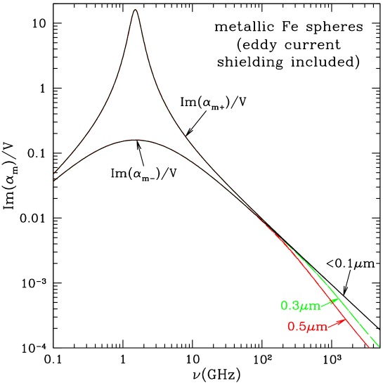
Figure 4: Dissipative part ${\rm Im}(\alpha_{\rm m})$ of magnetic polarizability arising from magnetization (solid curves) in Fe grains, including the shielding effects of eddy currents. The Gilbert equation with $\alpha_{\rm G}=0.2$ is assumed, and $\alpha_{\rm m}$ is shown for both circular polarizations. For $a\lesssim 0.3\micron$ eddy current shielding is unimportant for $\nu<500\,{\rm GHz}$.

5 Absorption by Small Particles: The Dipole Limit

For a uniform sphere illuminated by a monochromatic plane wave, the electromagnetic scattering problem can be solved exactly (Mie 1908; Debye 1909) provided the material is isotropic, i.e., can be characterized by a scalar dielectric function $\epsilon(\omega)$ and a scalar magnetic permeability $\mu(\omega)$. This mathematical solution is commonly referred to as “Mie theory”. Many numerical implementations of Mie theory assume the material to be nonmagnetic ($\mu=1$), although a code for general scalar $\epsilon$ and $\mu$ has been implemented by Milham (1994). The magnetic response (29) is, however, highly anisotropic, therefore the Mie theory solution is not directly applicable to the present problem. Lacking an exact solution, we seek an approximate treatment.

If the grain is small compared to $c/\omega$, then ${\bf E}_{\rm inc}$ and ${\bf H}_{\rm inc}$ can be approximated as uniform over the body of the grain. Let ${\bf p}_{\rm e}(t)$ and ${\bf p}_{\rm m}(t)$ be the electric and magnetic dipole moment of the grain. The time-averaged rate at which the incident wave does work on the grain is

$$\Bigl{\langle}\frac{dW}{dt}\Bigr{\rangle} = \Bigl{\langle}{\rm Re}({\bf E}_{\rm inc})\cdot\frac{d\,{\rm Re}({\bf p}_{\rm e})}{dt}\Bigr{\rangle}+\Bigl{\langle}{\rm Re}({\bf H}_{\rm inc})\cdot\frac{d\,{\rm Re}({\bf p}_{\rm m})}{dt}\Bigr{\rangle}$$ (69)

$$= \bigl{\langle}{\rm Re}({\bf E}_{\rm inc})\cdot{\rm Re}(-i\omega{\bf p}_{\rm e})\bigr{\rangle}+\bigl{\langle}{\rm Re}({\bf H}_{\rm inc})\cdot{\rm Re}(-i\omega{\bf p}_{\rm m})\bigr{\rangle}~{}~{}~{},$$ (70)

where $\langle...\rangle$ denotes a time-average. If $\hat{\bf e}_{j}$ and $\hat{\bf h}_{j}$ are normalized eigenvectors of ${\boldsymbol{\alpha}}_{\rm e}$ and ${\boldsymbol{\alpha}}_{\rm m}$, respectively, with eigenvalues $\alpha_{{\rm e},j}$ and $\alpha_{{\rm m},j}$ (for $j=1,2,3$) then (70) becomes

$$\Bigl{\langle}\frac{dW}{dt}\Bigr{\rangle}=\frac{\omega}{2}\sum_{j=1}^{3}\left[{\rm Im}(\alpha_{{\rm e},j})|{\bf E}_{\rm inc}^{*}\cdot\hat{\bf e}_{j}|^{2}+{\rm Im}(\alpha_{{\rm m},j})|{\bf H}_{\rm inc}^{*}\cdot\hat{\bf h}_{j}|^{2}\right]~{}~{}~{}.$$ (71)

For unpolarized, isotropic illumination, we set $|{\bf E}_{\rm inc}^{*}\cdot\hat{\bf e}_{j}|^{2}=(1/3)E_{0}^{2}$ and $|{\bf H}_{\rm inc}^{*}\cdot\hat{\bf h}_{j}|^{2}=(1/3)H_{0}^{2}=(1/3)E_{0}^{2}$. The absorption cross section is

$$\langle C_{\rm abs}\rangle = \frac{\langle dW/dt\rangle}{cE_{0}^{2}/8\pi}=\langle C_{\rm abs}^{\rm(e)}\rangle+\langle C_{\rm abs}^{\rm(mag)}\rangle$$ (72)

$$\langle C_{\rm abs}^{\rm(e)}\rangle = \frac{4\pi\omega}{3c}~{}{\rm Im}\left[{\rm Tr}({\boldsymbol{\alpha}}_{\rm e})\right]=\frac{\omega V}{3c}\sum_{j=1}^{3}\frac{\epsilon_{2}}{\left[(\epsilon_{1}-1)L_{j}+1\right]^{2}+\left[L_{j}\epsilon_{2}\right]^{2}}$$ (73)

$$\langle C_{\rm abs}^{\rm(mag)}\rangle = \frac{4\pi\omega}{3c}~{}{\rm Im}\left[{\rm Tr}({\boldsymbol{\alpha}}_{\rm m})\right]=\frac{4\pi\omega V}{3c}{\rm Im}\left(\chi_{+}+\chi_{-}\right)+\frac{4\pi\omega}{c}{\rm Im}\left(\alpha_{\rm m}^{\rm(eddy)}\right)~{}~{}~{},$$ (74)

where ${\rm Tr}$ denotes the trace of a matrix, equivalent to the sum of eigenvalues.

6 Magnetic Absorption Cross Section

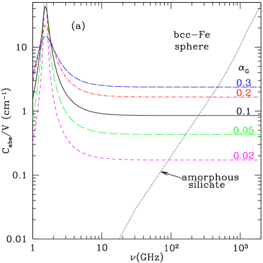
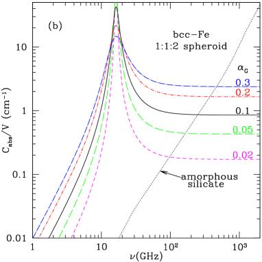
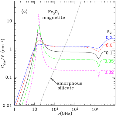
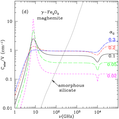
Figure 5: Magnetic absorption cross section $C_{\rm abs}$ per volume $V$ calculated from (74) for (a) Fe sphere, (b) Fe 1.5:1 prolate spheroid, (c) Fe₃O₄ magnetite, and (d) $\gamma$-Fe₂O₃ maghemite (see text). For ferrimagnetic materials, $C_{\rm abs}/V$ is shape-independent. For comparison, the dotted line shows $C_{\rm abs}/V$ for small spheres of amorphous silicate.

6.1 Ferromagnetic Material

For a ferromagnetic material with $\chi_{\pm}$ given by (26), we have

$$\bigl{\langle}C_{\rm abs}^{\rm(mag)}(\omega)\bigr{\rangle} = \frac{8\pi}{3}\frac{V}{c}\frac{\alpha_{\rm G}\omega^{2}\omega_{M}\left[\omega_{0}^{2}+(1+\alpha_{\rm G}^{2})\omega^{2}\right]}{\left[\omega_{0}^{2}-(1+\alpha_{\rm G}^{2})\omega^{2}\right]^{2}+4\alpha_{\rm G}^{2}\omega_{0}^{2}\omega^{2}}~{}~{}~{}.$$ (75)

with a peak near

$$\omega_{{\rm res},+}\equiv\frac{\omega_{0}}{\sqrt{1+\alpha_{\rm G}^{2}}}\approx\omega_{0}$$ (76)

The resonance at $\omega_{{\rm res},+}$ is associated with the $\hat{\bf h}_{+}$ circular polarization mode. The height and width of the resonant absorption are determined by the damping coefficient $\alpha_{\rm G}$. The resonance frequency $\omega_{{\rm res},+}$ depends on the eigenvalues of the demagnetization tensor ${\bf D}$ (see eq. 15), and hence on the particle shape. Table 2 gives $\omega_{0}$ for Fe spheres and spheroids with selected shapes. Figures 5a and 5b show $C_{\rm abs}/V$ for Fe spheres (absorption peak at $\sim$$1.5\,{\rm GHz}$) and 2:1 prolate spheroids (absorption peak at $\sim$$16\,{\rm GHz}$).

The asymptotic behavior for ferromagnetic material is

$$\langle C_{\rm abs}^{\rm(mag)}\rangle\rightarrow\left\{\begin{array}[]{l l}\frac{8\pi V}{3c}\frac{\alpha_{\rm G}\omega_{M}\omega^{2}}{\omega_{0}^{2}}&{\rm for~{}}\omega\ll\omega_{0}\\ \frac{8\pi V}{3c}\frac{\alpha_{\rm G}\omega_{M}}{(1+\alpha_{G}^{2})}&{\rm for~{}}\omega\gg\omega_{0}\end{array}\right.~{}~{}~{}.$$ (77)

6.2 Ferrimagnetic Material

For ferrimagnetic materials, with $\chi_{\pm}$ given by (59), $C_{\rm abs}(\omega)$ has more complicated behavior. For $\alpha_{\rm G}\ll 1$ there are two local extrema, near

$$\omega_{{\rm res},\pm}=\left[\frac{(\omega_{0A}+\omega_{0B})^{2}}{4}-\omega_{0A}\omega_{0B}+N_{AB}^{2}\omega_{MA}\omega_{MB}\right]^{1/2}\pm\frac{(\omega_{0A}+\omega_{0B})}{2}~{}~{}~{}.$$ (78)

The frequency $\omega_{{\rm res},+}$ for resonance when ${\bf h}\propto\hat{\bf h}_{+}$ (i.e., applied field rotating anticlockwise around the static magnetization ${\bf M}$) is the frequency of free precession of the magnetizations ${\bf M}_{A}$ and ${\bf M}_{B}$ around the $\hat{\bf z}$ axis, with ${\bf M}_{A}$ and ${\bf M}_{B}$ remaining antiparallel – it corresponds to ordinary ferromagnetic resonance, with ${\bf m}_{A}=-\beta{\bf m}_{B}$.

The frequency $\omega_{{\rm res},-}$ associated with polarization $\hat{\bf h}_{-}$ is much higher – at THz frequencies – and corresponds to precession with ${\bf M}_{B}$ and ${\bf M}_{A}$ no longer antiparallel, but instead with ${\rm Re}({\bf m}_{A})\cdot{\rm Re}({\bf m}_{B})>0$. With ${\bf M}_{A}$ and ${\bf M}_{B}$ no longer antiparallel, the precession is driven primarily by the strong coupling $N_{AB}{\bf M}_{A}\cdot{\bf M}_{B}$.

The asymptotic behavior for ferrimagnetic material is

$$\langle C_{\rm abs}^{\rm(mag)}\rangle\rightarrow\left\{\begin{array}[]{l l}\frac{8\pi V}{3c}\alpha_{\rm G}A\omega^{2}&{\rm for~{}}\omega\ll\omega_{{\rm res},+}\\ \frac{8\pi V}{3c}\alpha_{\rm G}B&{\rm for~{}}\omega\gg\omega_{{\rm res},-}\end{array}\right.~{}~{}~{},$$ (79)

where

$$A\equiv\frac{(2N_{AB}\omega_{MA}\omega_{MB}-\omega_{MA}\omega_{0B}-\omega_{MB}\omega_{0A})(\omega_{0B}\!-\!\omega_{0A})}{\left(N_{AB}^{2}\omega_{MA}\omega_{MB}-\omega_{0A}\omega_{0B}\right)^{2}}-\frac{(\omega_{MB}-\omega_{MA})}{(N_{AB}^{2}\omega_{MA}\omega_{MB}-\omega_{0A}\omega_{0B})}$$ (80)

$$B\equiv\frac{(\omega_{MB}-\omega_{MA})}{(1+\alpha_{\rm G}^{2})}~{}~{}~{}.$$ (81)

Figures 5c and 5d show the magnetic contribution to the absorption cross section per unit volume calculated for small particles of magnetite Fe₃O₄, and maghemite $\gamma$-Fe₂O₃.

The dip in absorption at the upper resonance frequency $\omega_{{\rm res},-}$ is notable in Figures 5c and 5d, but we will see below that at these frequencies electric dipole absorption is dominant, and this feature in the magnetic dipole absorption is probably not observable.

7 Opacities

Above we have discussed the response of metallic Fe, magnetite, and maghemite to oscillating electric and magnetic fields in the dipole limit, $a\ll\lambda$. We now calculate the absorption cross section, as a function of wavelength, including both electric and magnetic effects, over a broad range of frequencies.

We will treat the grains as spherical and calculate $C_{\rm abs}^{\rm MT}$ using Mie theory with $\mu=1$. To this we add the magnetic dipole absorption calculated in the magnetic dipole limit, including the eddy current correction. Thus, for randomly-oriented grains, we take

$$C_{\rm abs}=C_{\rm abs}^{\rm MT}+\frac{4\pi\omega V}{3c}{\rm Im}\left[\left(1-\phi_{\rm eddy}\right)\left(\chi_{+}+\chi_{-}\right)\right]~{}~{}~{}.$$ (82)

The magnetization response for Fe is strongly dependent on the shape of the Fe particles. Interstellar Fe nanoparticles – whether free-flying or inclusions within larger grains – are presumably nonspherical. To compute the magnetization contribution to the absorption, we will assume the Fe to be in 2:1 prolate spheroids (magnetized along the symmetry axis).

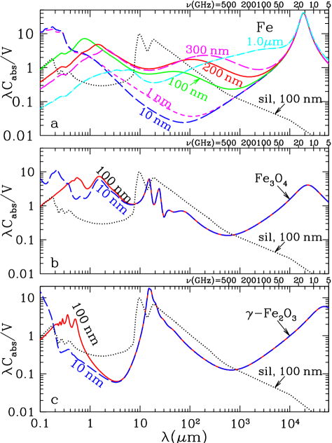
Figure 6: $\lambda C_{\rm abs}/V$ as a function of wavelength $\lambda$. (a) Fe spheres with radii $a=1$, 10, 100, 200, 300, and $10^{3}\,{\rm nm}$. The increase in opacity near $\lambda=100\micron$ as $a$ increases from $10\,{\rm nm}$ to $300\,{\rm nm}$ is due to the increased dissipation by eddy currents. The eddy current absorption peak shifts to longer wavelengths with increasing grain size. For $a<100\,{\rm nm}$, absorption for $\lambda>1000\micron$ ($\nu<300\,{\rm GHz}$) is dominated by magnetic absorption, with a ferromagnetic resonance peak at $\sim$$15\,{\rm GHz}$ (the ferromagnetic absorption has been calculated for 2:1 prolate spheroids – see text). (b) Magnetite spheres with radii $a=10$ and $100\,{\rm nm}$. The ferrimagnetic resonance peak is at $15\,{\rm GHz}$. (c) Maghemite spheres with radii $a=10$ and $100\,{\rm nm}$. Because of the low electrical conductivity, eddy current absorption is unimportant for magnetite and maghemite. The ferrimagnetic resonance peak is at $8\,{\rm GHz}$. Also shown is $\lambda C_{\rm abs}/V$ for $a=100\,{\rm nm}$ amorphous silicate spheres.

Figure 6a shows $\lambda C_{\rm abs}/V$ as a function of $\lambda$ for Fe spheres with selected radii ranging from $a=1\,{\rm nm}$ to $1.0\micron$. For comparison, we also show $\lambda C_{\rm abs}/V$ for $a=100\,{\rm nm}$ amorphous silicate spheres. Because amorphous silicate is nonconducting, electric dipole absorption dominates in the FIR, and $C_{\rm abs}^{\rm(e)}/V$ is independent of $a$ for $2\pi a/\lambda\ll 1$. By contrast, the eddy current absorption in the Fe particles causes $C_{\rm abs}^{\rm(mag)}/V$ at far-infrared and submm frequencis to be sensitive to $a$ (see also Figure 4). For $a\gtrsim 100\,{\rm nm}$, “magnetic dipole” absorption due to eddy current dissipation is important for $\lambda\gtrsim 30\micron$. True magnetic absorption dominates only at very long wavelengths: for $a=100\,{\rm nm}$, magnetic absorption dominates for $\lambda>1\,$mm ($\nu<300\,{\rm GHz}$).

From Figure 6a we see that at $\lambda=10^{3}\micron=1\,{\rm mm}$ ($\nu=300\,{\rm GHz}$) an $a=100\,{\rm nm}$ Fe sphere has $C_{\rm abs}/V$ that is a factor $\sim$2 times larger than for astrosilicate, whereas for $a=300\,{\rm nm}$, $C_{\rm abs}/V$ exceeds astrosilicate by a factor $\sim$10, because of eddy currents in the conducting particle. Therefore, if a significant fraction of the interstellar Fe is in particles of such size, it could noticeably affect the overall submm and mm-wave emission.

8 Grain Temperatures

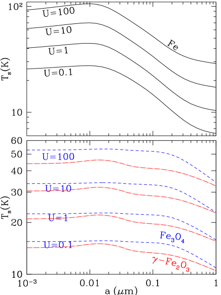
Figure 7: Steady-state temperature $T_{s}$ as a function of radius $a$ for spheres of Fe, Fe₃O₄, and Fe₂O₃ grains heated by radiation with the spectrum of the local ISRF (Mathis et al. 1983) and intensity $U=0.1,1,10,10^{2}$ times that of the local ISRF.

With absorption cross sections $C_{\rm abs}(\omega)$ calculated as described above, we can evaluate the rate

$$P_{\rm heat}(a)=\int d\nu\,C_{\rm abs}(\nu)u_{\nu}c$$ (83)

at which a grain of radius $a$ will absorb energy from the interstellar radiation field with specific energy density $u_{\nu}$. We assume $u_{\nu}$ to have the spectrum estimated by Mathis et al. (1983, herafter MMP83) for the local interstellar radiation field (ISRF) multiplied by a factor $U$ ($U=1$ corresponds to the solar-neighborhood ISRF). We then solve for the “steady-state” temperature $T_{s}$ for which the time-averaged thermal emission is equal to $P_{\rm heat}$:

$$\int d\nu\,C_{\rm abs}(\nu)4\pi B_{\nu}(T_{s})=P_{\rm heat}~{}~{}~{}.$$ (84)

The actual grain temperature will fluctuate around $T_{s}$. For $a\gtrsim 0.01\micron$ the temperature fluctuations are small enough that they can be neglected here.

Figure 7 shows the steady-state grain temperature $T_{s}$ as a function of radius $a$ for Fe, magnetite, and maghemite grains heated by radiation with the MMP83 spectrum.

9 Infrared Emission Spectrum

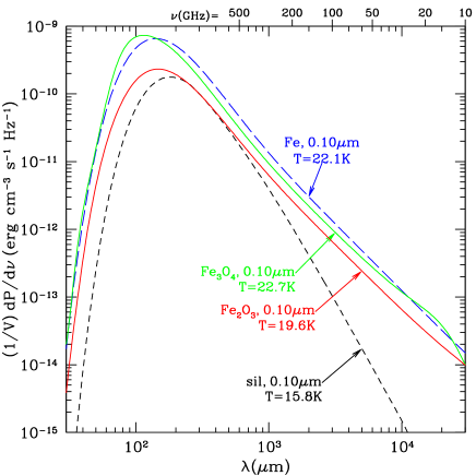
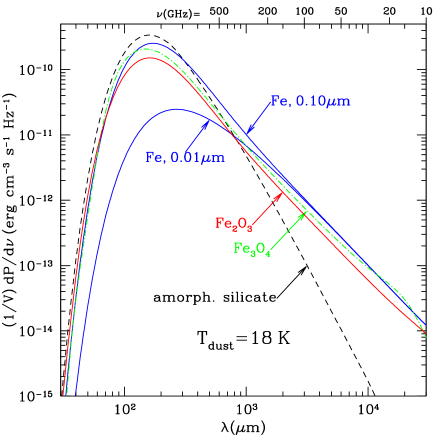
Figure 8: (a) Emissivity per grain volume of $a=0.10\micron$ grains of astrosilicate, metallic Fe, magnetite Fe₃O₄, and maghemite $\gamma-$Fe₂O₃, heated by the MMP83 radiation field. (b) Emissivity per grain volume of small grains of astrosilicate, metallic Fe, magnetite, and maghemite at $T=18\,{\rm K}$.

Figure 8a shows the emission spectrum, per unit grain volume, for $a=0.1\micron$ spheres of Fe, Fe₃O₄, and $\gamma$-Fe₂O₃ heated by the MMP83 starlight spectrum with the intensity ($U=1$) estimated for the Solar neighborhood. Because of their enhanced absorption cross sections in the optical and near-IR, the Fe, Fe₃O₄, and $\gamma$-Fe₂O₃ grains are somewhat warmer than amorphous silicate grains heated by the same $U=1$ radiation fields, with grain temperatures of $\sim$20K versus the 15.8K temperature for the amorphous silicate grain, but all have emission spectra peaking near $\sim$150$\micron$. At longer wavelengths $\lambda\gtrsim 1\,{\rm mm}$ ($\nu<300\,{\rm GHz}$), the magnetic grains radiate more strongly than the amorphous silicate, as expected from the cross sections shown in Figure 6.

The magnetic grains may be inclusions in larger grains (rather than free-fliers), in which case it is more appropriate to compare the emissivities of the different grain materials at a common temperature. Figure 8b shows the emission per unit grain volume at $T=18\,{\rm K}$ for the same four grain materials. At 300 GHz ($\lambda=10^{3}\micron$), the power radiated per grain volume by the magnetic grains ranges from 1.2 (for $\gamma$-Fe₂O₃) to 2.2 (for Fe₃O₄) times larger than the emission from the amorphous silicate. At 100 GHz the difference between amorphous silicate and the magnetic materials is even more pronounced: factors of 5 (for $\gamma$-Fe₂O₃), 8 (for Fe₃O₄) and 9 (for Fe).

10 Polarization

10.1 Davis-Greenstein Alignment

Let ${\bf h}_{\rm ism}$ be the static interstellar magnetic field; ${\bf h}_{\rm ism}$ is very weak compared to either $4\pi{\bf M}_{0}$ or the crystalline anisotropy field ${\bf H}_{K}$. However, as pointed out by Davis & Greenstein (1951), ${\bf h}_{\rm ism}$ can exert systematic torques on a spinning grain.

Consider a magnetic particle spinning in space at some rotational frequency ${\boldsymbol{\omega}}$. Grain rotation can be excited by many processes. At a minimum, elastic collisions with gas atoms will excite “Brownian” rotation with

$$\frac{\omega}{2\pi}\approx\frac{1}{2\pi}\left(\frac{15kT}{8\pi\rho a^{5}}\right)^{1/2}\approx 20\,{\rm kHz}\left(\frac{T}{10^{2}\,{\rm K}}\right)^{1/2}\left(\frac{5\,{\rm g}\,{\rm cm}^{-3}}{\rho}\right)^{1/2}\left(\frac{0.1\micron}{a}\right)^{5/2}~{}~{}~{}.$$ (85)

However, grains with $a\gtrsim 0.1\micron$ appear likely to be spinning suprathermally, as a result of systematic torques due to formation of ${\rm H}_{2}$ on the grain surface and emission of photoelectrons (Purcell 1979) as well as radiative torques due to starlight (Draine & Weingartner 1996). Suprathermal rotation of small $a\lesssim 0.05\micron$ grains is thought to be suppressed by “thermal flipping” (Lazarian & Draine 1999).

Let $\psi$ be the angle between ${\boldsymbol{\omega}}$ and ${\bf h}_{\rm ism}$. The grain’s spontaneous magnetization ${\bf M}_{0}$ need not be aligned with its angular velocity ${\boldsymbol{\omega}}$; let $\Theta$ be the angle between ${\bf M}_{0}$ and ${\boldsymbol{\omega}}$. Let $\hat{\bf x}_{m}$, $\hat{\bf y}_{m}$, $\hat{\bf z}_{m}$ be unit vectors “frozen into” the magnetic material, with $\hat{\bf z}_{m}\parallel{\bf M}_{0}$. The magnetic field can be separated into two components, one that appears stationary to the rotating grain, and another, denoted ${\bf h}_{{\rm ism},\omega}$, oscillating with frequency $\omega$. Choose $\hat{\bf x}_{m}$ to be perpendicular to the ${\boldsymbol{\omega}}-{\bf M}_{0}$ plane, and $\hat{\bf y}_{m}=\hat{\bf z}_{m}\times\hat{\bf x}_{m}$. If ${\rm Re}({\bf h}_{{\rm ism},\omega})$ is in the $\hat{\bf x}_{m}$ direction at $t=0$ then the magnetic field in “grain coordinates” is

$${\bf h}_{\rm ism} = h_{\rm ism}\cos\psi\cos\Theta\,\hat{\bf z}_{m}+{\rm Re}\left({\bf h}_{{\rm ism},\omega}\right)$$ (86)

$${\bf h}_{{\rm ism},\omega} = h_{\rm ism}\sin\psi~{}\left(-\hat{\bf x}_{m}+i\cos\Theta\,\hat{\bf y}_{m}-i\sin\Theta\,\hat{\bf z}_{m}\right)e^{-i\omega t}~{}~{}~{}.$$ (87)

The grain is spinning in a static field. Following Davis & Greenstein, assume that the magnetic dissipation in the grain material is the same as in a stationary sample in a rotating magnetic field corresponding to ${\bf h}_{{\rm ism},\omega}$. As before, the magnetic eigenmodes are $\hat{\bf h}_{\pm}=(\hat{\bf x}_{m}\pm i\hat{\bf y}_{m})/\sqrt{2}$, and the time-averaged energy dissipation rate is (see eq. 70)

$$\Bigl{\langle}\frac{dW}{dt}\Bigr{\rangle} = \frac{\omega}{2}V\left[{\rm Im}(\chi_{+})|{\bf h}_{{\rm ism},\omega}\cdot\hat{\bf h}_{+}^{*}|^{2}+{\rm Im}(\chi_{-})|{\bf h}_{{\rm ism},\omega}\cdot\hat{\bf h}_{-}^{*}|^{2}\right]$$ (88)

$$= \frac{1}{4}\omega Vh_{\rm ism}^{2}\sin^{2}\psi\left[(1-\cos\Theta)^{2}{\rm Im}(\chi_{+})+(1+\cos\Theta)^{2}{\rm Im}(\chi_{-})\right]$$ (89)

$$\approx \frac{1}{2}\omega Vh_{\rm ism}^{2}\sin^{2}\psi\left(1+\cos^{2}\Theta\right){\rm Im}\left(\frac{\chi_{+}+\chi_{-}}{2}\right)$$ (90)

$$= KVh_{\rm ism}^{2}\omega^{2}\sin^{2}\psi$$ (91)

$$K(\Theta) \equiv \frac{{\rm Im}(\chi_{+}+\chi_{-})}{2\omega}~{}\left(\frac{1+\cos^{2}\Theta}{2}\right)$$ (92)

$$\approx \frac{\alpha_{\rm G}\omega_{M}}{2\omega_{0}^{2}}(1+\cos^{2}\Theta)~{}~{}~{},$$ (93)

where the approximation (90) takes ${\rm Im}(\chi_{+}-\chi_{-})\ll{\rm Im}(\chi_{+}+\chi_{-})$ because the grain rotational frequency $\omega\ll\omega_{0}$.

The grain, spinning in a static field, is converting rotational kinetic energy into heat. Davis and Greenstein showed that the associated torques would act to reduce the transverse component of the angular momentum, bringing the grain rotation axis into alignment with the local magnetic field. If $K$ is constant, the dissipation causes $\tan\psi$ to decay exponentially:

$$\tan\psi = \tan\psi(t=0)~{}e^{-t/\tau_{\rm DG}}$$ (94)

$$\tau_{\rm DG} = \frac{I}{VKh_{\rm ism}^{2}}\approx\frac{2\rho a^{2}}{5Kh_{\rm ism}^{2}}$$ (95)

$$= 5.1\times 10^{5}\,{\rm yr}\left(\frac{\rho}{5\,{\rm g}\,{\rm cm}^{-3}}\right)\left(\frac{a}{0.1\micron}\right)^{2}\left(\frac{10^{-13}\,{\rm s}}{K}\right)\left(\frac{5\mu{\rm G}}{h_{\rm ism}}\right)^{2}~{}~{}~{},$$ (96)

where $I$ is the moment of inertia. For metallic Fe in a 2:1 prolate spheroid,

$$K\approx 1.47\times 10^{-12}\alpha_{\rm G}(1+\cos^{2}\Theta)\,{\rm s}~{}~{}~{}.$$ (97)

If $\alpha_{\rm G}\approx 0.2$, this gives a rate of magnetic dissipation that is only slightly larger than what is estimated for normal paramagnetic materials, $K\approx 10^{-13}(18\,{\rm K}/T_{\rm gr})\,{\rm s}$ (Jones & Spitzer 1967). However, as discussed in Appendix A, at low or intermediate frequencies, we might expect the effective value of $\alpha_{\rm G}$ to be $\alpha_{\rm G}\approx 1/\omega\tau_{2}$, where $\tau_{2}$ is the spin-spin relaxation time. For a typical spin-spin relaxation time of $\sim 10^{-10}\,{\rm s}$, we would then have $\alpha_{\rm G}\approx 8\times 10^{4}[20\,{\rm kHz}/(\omega/2\pi)](10^{-10}\,{\rm s}/\tau_{2})$, suggesting that $K\sim 10^{-7}\,{\rm s}$ for grains where metallic Fe is a significant fraction of the grain volume, giving a Davis-Greenstein alignment time $\tau_{\rm DG}\approx 1\,{\rm yr}$: extremely rapid alignment of the grain angular momentum with the local magnetic field.

Rapid alignment by ferromagnetic inclusions, originally proposed by Jones & Spitzer (1967), has been previously discussed by various authors, including Duley (1978), Mathis (1986), Goodman & Whittet (1995), and Martin (1995).

10.2 Polarization of the Magnetic Dipole Emission

10.2.1 Single-Domain Magnetic Grains

Single-domain magnetic grains, if their directions of static magnetization are aligned, will produce strong polarization, as previously noted by DL99. Let us assume that the grains are prolate spheroids, magnetized along the long axis. The grains are assumed to be spinning around an axis perpendicular to the symmetry axis. Without loss of generality, let $\hat{\bf x}$ point toward the observer, let $\hat{\bf z}$ be orthogonal to $\hat{\bf x}$ and ${\bf H}_{0}$, and let $\hat{\bf y}=\hat{\bf z}\times\hat{\bf x}$. Then ${\bf H}_{0}$ is in the $\hat{\bf x}\hat{\bf y}$ plane.

Figure 9: Degree of linear polarization for magnetic dipole emission from free-flying, partially-aligned single-domain magnetic grains, as a function of the angle $\Phi$ between the line-of-sight and the magnetic field ${\bf H}_{0}$ defining the alignment direction. Results are shown for perfect alignment $\langle\cos^{2}\psi\rangle=1$, and partial alignment with $\langle\cos^{2}\psi\rangle=0.5$. The polarization is zero for random alignment ($\langle\cos^{2}\psi\rangle=1/3$), and negative for $\langle\cos^{2}\psi\rangle<1/3$.

If $\hat{\bf z}_{\rm m}$ is a unit vector along the prolate symmetry axis (the direction of magnetization), then the magnetic absorption cross section for linearly-polarized radiation with ${\bf H}_{\rm inc}=H_{\rm inc}\hat{\bf h}e^{-i\omega t}$ can be written

$$C_{\rm abs}^{\rm(mag)}=\frac{2\pi}{c}\omega V{\rm Im}(\chi_{+}+\chi_{-})\left[1-\langle(\hat{\bf h}\cdot\hat{\bf z}_{\rm m})^{2}\rangle\right]~{}~{}~{}.$$ (98)

The brackets $\langle...\rangle$ denote averaging over the grain rotation and precession. Let $C_{{\rm abs},\perp}$ and $C_{{\rm abs},\parallel}$ be $C_{\rm abs}$ for ${\bf E}_{\rm inc}\perp\hat{\bf y}$ (i.e., ${\bf H}_{\rm inc}\parallel\hat{\bf y}$) and ${\bf E}_{\rm inc}\parallel\hat{\bf y}$ (i.e., ${\bf H}_{\rm inc}\parallel\hat{\bf z}$), respectively:

$$C_{{\rm abs},\perp}^{\rm(mag)} = \frac{2\pi}{c}\omega V{\rm Im}(\chi_{+}+\chi_{-})\left[1-\langle(\hat{\bf y}\cdot\hat{\bf z}_{\rm m})^{2}\rangle\right]$$ (99)

$$C_{{\rm abs},\parallel}^{\rm(mag)} = \frac{2\pi}{c}\omega V{\rm Im}(\chi_{+}+\chi_{-})\left[1-\langle(\hat{\bf z}\cdot\hat{\bf z}_{\rm m})^{2}\rangle\right]~{}~{}~{}.$$ (100)

The fractional polarization of the emitted radiation is just

$$p = \frac{C_{{\rm abs},\perp}^{\rm(mag)}-C_{{\rm abs},\parallel}^{\rm(mag)}}{C_{{\rm abs},\perp}^{\rm(mag)}+C_{{\rm abs},\parallel}^{\rm(mag)}}$$ (101)

$$= \frac{\langle(\hat{\bf z}\cdot\hat{\bf z}_{\rm m})^{2}\rangle-\langle(\hat{\bf y}\cdot\hat{\bf z}_{\rm m})^{2}\rangle}{2-\langle(\hat{\bf z}\cdot\hat{\bf z}_{\rm m})^{2}\rangle-\langle(\hat{\bf z}\cdot\hat{\bf z}_{\rm m})^{2}\rangle}~{}~{}~{}.$$ (102)

Let $\Phi$ be the angle between the line-of-sight $\hat{\bf x}$ and ${\bf H}_{0}$, and let $\psi$ be the “alignment angle” between the grain angular momentum (assumed to be $\perp$ to the long axis) and ${\bf H}_{0}$. Then (see Appendix E)

$$p=\frac{\sin^{2}\Phi\left(3\langle\cos^{2}\psi\rangle-1\right)}{5+\langle\cos^{2}\psi\rangle\left(1-3\cos^{2}\Phi\right)}~{}~{}~{}.$$ (103)

The numerator is proportional to the familiar “Rayleigh reduction factor” $(3/2)(\langle\cos^{2}\psi\rangle-1/3)$, which varies from 0 to 1 as $\langle\cos^{2}\psi\rangle$ varies from $1/3$ to 1. The polarization $p$ is plotted as a function of $\Phi$ in Figure 9, for selected values of $\langle\cos^{2}\psi\rangle$, including 1 (perfect alignment), $1/3$ (random alignment), and $\langle\cos^{2}\psi\rangle=0$ (perfect antialignment).

Single-domain grains aligned with the long axis (and magnetization) ${\bf z}_{\rm m}\perp{\bf H}_{0}$ give $p>0$. The assumed perfect alignment of the grain’s magnetization with the principal axis of smallest moment of inertia results in very large polarizations, ranging from $-0.2$ to $1/3$ depending on the values of $\langle\cos^{2}\psi\rangle$ and $\sin^{2}\Phi$.

10.2.2 Randomly-Oriented Magnetic Inclusions

Magnetic material might be primarily in the form of “inclusions” in larger grains. If the nonspherical inclusions are themselves perfectly oriented relative to the principal axes of the host grain, then (103) will approximate the polarization of the magnetic dipole emission.

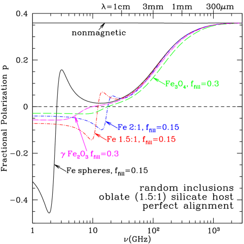
Figure 10: Degree of linear polarization for emission from perfectly aligned 1.5:1 oblate spheroids composed of amorphous silicate only (curve labelleled “nonmagnetic”) or amorphous silicate grains with randomly-oriented single-domain magnetic inclusions. Magnetic inclusions considered are Fe spheres and spheroids (1.5:1 and 2:1) with volume filling factor $f_{\rm fill}=0.15$, Fe₃O₄ magnetite with $f_{\rm fill}=0.3$, and $\gamma$-Fe₂O₃ maghemite with $f_{\rm fill}=0.3$. At high frequencies, electric dipole emission dominates, polarized with ${\bf E}$ along the long axes ($p>0$). For grains with magnetic inclusions, magnetic dipole emission dominates at low frequency, polarized with ${\bf H}$ along the long axes ($p<0$). The detailed frequency dependence depends on the nature of the magnetic inclusions, but in all cases the degree of polarization drops by a factor $\sim$4 as the frequency is reduced from $300\,{\rm GHz}$ to $50\,{\rm GHz}$.

If, as seems more likely, the inclusions are randomly-oriented relative to the principal axes of the host, and the inclusions have a sufficiently low volume filling factor $f_{\rm fill}$, then, using effective medium theory (see Appendix F) we may approximate the magnetic permeability of the grain as a sum over the magnetic response of the individual inclusions (assumed to be spherical – see eq. F10):

$$\mu\approx 1+f_{\rm fill}\frac{4\pi}{3}\left(\chi_{+}+\chi_{-}\right)~{}~{}~{}.$$ (104)

The host material is assumed to be nonmagnetic. For simplicity, we let both inclusions and host have the same complex dielectric function $\epsilon(\omega)$. We assume the grain to be spinning around $\hat{\bf a}_{1}$, the principal axis of largest moment of inertia; ${\boldsymbol{\omega}}$ precesses around ${\bf H}_{\rm ism}$, with an angle $\psi$ between ${\boldsymbol{\omega}}$ and ${\bf H}_{\rm ism}$. Let $\Phi$ be the angle between the static magnetic field and the line-of-sight. For a grain with shape factors $L_{1},L_{2},L_{3}$ (for principal axes $\hat{\bf a}_{1}$, $\hat{\bf a}_{2}$, $\hat{\bf a}_{3}$), the absorption cross section in the dipole limit is

$$C_{{\rm abs},\perp} = V\frac{\omega}{c}\bigg{[}{\rm Im}(\epsilon)\left(\frac{\langle(\hat{\bf z}\cdot\hat{\bf a}_{1})^{2}\rangle}{|1+L_{1}(\epsilon-1)|^{2}}+\frac{\langle(\hat{\bf z}\cdot\hat{\bf a}_{2})^{2}\rangle}{|1+L_{2}(\epsilon-1)|^{2}}+\frac{\langle(\hat{\bf z}\cdot\hat{\bf a}_{3})^{2}\rangle}{|1+L_{3}(\epsilon-1)|^{2}}\right)+$$ (105)

$$\hskip 20.00003pt{\rm Im}(\mu)\left(\frac{\langle(\hat{\bf y}\cdot\hat{\bf a}_{1})^{2}\rangle}{|1+L_{1}(\mu-1)|^{2}}+\frac{\langle(\hat{\bf y}\cdot\hat{\bf a}_{2})^{2}\rangle}{|1+L_{2}(\mu-1)|^{2}}+\frac{\langle(\hat{\bf y}\cdot\hat{\bf a}_{3})^{2}\rangle}{|1+L_{3}(\mu-1)|^{2}}\right)\bigg{]}$$

$$C_{{\rm abs},\parallel} = V\frac{\omega}{c}\bigg{[}{\rm Im}(\epsilon)\left(\frac{\langle(\hat{\bf y}\cdot\hat{\bf a}_{1})^{2}\rangle}{|1+L_{1}(\epsilon-1)|^{2}}+\frac{\langle(\hat{\bf y}\cdot\hat{\bf a}_{2})^{2}\rangle}{|1+L_{2}(\epsilon-1)|^{2}}+\frac{\langle(\hat{\bf y}\cdot\hat{\bf a}_{3})^{2}\rangle}{|1+L_{3}(\epsilon-1)|^{2}}\right)+$$ (106)

$$\hskip 20.00003pt{\rm Im}(\mu)\left(\frac{\langle(\hat{\bf z}\cdot\hat{\bf a}_{1})^{2}\rangle}{|1+L_{1}(\mu-1)|^{2}}+\frac{\langle(\hat{\bf z}\cdot\hat{\bf a}_{2})^{2}\rangle}{|1+L_{2}(\mu-1)|^{2}}+\frac{\langle(\hat{\bf z}\cdot\hat{\bf a}_{3})^{2}\rangle}{|1+L_{3}(\mu-1)|^{2}}\right)\bigg{]}~{}~{},~{}~{}~{}~{}$$

where the orientational averages are (see Appendix E)

$$\langle(\hat{\bf y}\cdot\hat{\bf a}_{1})^{2}\rangle = \sin^{2}\Phi\langle\cos^{2}\psi\rangle+\frac{1}{2}\cos^{2}\Phi\langle\sin^{2}\psi\rangle$$ (107)

$$\langle(\hat{\bf y}\cdot\hat{\bf a}_{2})^{2}\rangle=\langle(\hat{\bf y}\cdot\hat{\bf a}_{3})^{2}\rangle = \frac{1}{4}\cos^{2}\Phi(1+\langle\cos^{2}\psi\rangle)+\frac{1}{2}\sin^{2}\Phi\langle\sin^{2}\psi\rangle$$ (108)

$$\langle(\hat{\bf z}\cdot\hat{\bf a}_{1})^{2}\rangle = \frac{1}{2}\langle\sin^{2}\psi\rangle$$ (109)

$$\langle(\hat{\bf z}\cdot\hat{\bf a}_{2})^{2}\rangle=\langle(\hat{\bf z}\cdot\hat{\bf a}_{3})^{2}\rangle = \frac{1}{4}\left(1+\langle\cos^{2}\psi\rangle\right)~{}~{}~{}.$$ (110)

The fractional polarization of the emission is

$$p \equiv \frac{C_{{\rm abs},\perp}-C_{{\rm abs},\parallel}}{C_{{\rm abs},\perp}+C_{{\rm abs},\parallel}}=\frac{2N}{D}[1+3\cos(2\psi)]\sin^{2}\Phi$$ (111)

$$N = B_{1}B_{2}B_{3}\left[A_{1}(A_{2}+A_{3})-2A_{2}A_{3}\right]{\rm Im}(\epsilon)-$$ (112)

$$A_{1}A_{2}A_{3}\left[B_{1}(B_{2}+B_{3})-2B_{2}B_{3}\right]{\rm Im}(\mu)$$

$$D = \Big{\{}10A_{2}A_{3}+11A_{1}(A_{2}+A_{3})+$$ (113)

$$\left[A_{1}(A_{2}+A_{3})-2A_{2}A_{3}\right]\left(\cos(2\psi)+\cos(2\Phi)\left[1+3\cos(2\psi)\right]\right)\Big{\}}B_{1}B_{2}B_{3}{\rm Im}(\epsilon)+$$

$$\Big{\{}10B_{2}B_{3}+11B_{1}(B_{2}+B_{3})+$$

$$\left[B_{1}(B_{2}+B_{3})-2B_{2}B_{3}\right]\left(\cos(2\psi)+\cos(2\Phi)\left[1+3\cos(2\psi)\right]\right)\Big{\}}A_{1}A_{2}A_{3}{\rm Im}(\mu)$$

$$A_{j} \equiv |1+L_{j}(\epsilon-1)|^{2}$$ (114)

$$B_{j} \equiv |1+L_{j}(\mu-1)|^{2}$$ (115)

What volume filling factors might be expected? Forsterite Mg₂SiO₄ ($\rho=3.25\,{\rm g}\,{\rm cm}^{-3}$) has a volume per Mg $V_{\rm Mg}=3.6\times 10^{-23}\,{\rm cm}^{3}$. Solar abundances have Mg/Fe$\approx 1.26$ (Asplund et al. 2009). Thus if all of the Mg were in Mg₂SiO₄, and all of the Fe were in magnetic inclusions, the volume filling factor of the inclusions would be $f_{\rm fill}=V_{\rm Fe}/(1.26V_{\rm Mg}+V_{\rm Fe})=0.20$ for metallic Fe, $0.35$ for Fe₃O₄, and $0.38$ for $\gamma$-Fe₂O₃ (using the values for $V_{\rm Fe}$ from Table 1).

Figure 10 shows $p$ calculated using eqs. (106-111) for 1.5:1 oblate spheroids ($L_{1}=0.446$, $L_{2}=L_{3}=0.277$) of amorphous silicate, containing randomly-oriented magnetic inclusions with volume filling factor $f_{\rm fill}=0.15$ for metallic Fe, or $f_{\rm fill}=0.3$ for Fe₃O₄ or $\gamma$-Fe₂O₃. Electric dipole emission dominates at high frequencies, and (for perfect alignment) $p$ is large, $p\gtrsim 0.2$. With decreasing frequency, the importance of the magnetic dipole contribution increases and $p$ decreases. For all of the examples with magnetic inclusions, $p$ decreases by a factor $\sim$4 as the frequency varies from $300\,{\rm GHz}$ to $50\,{\rm GHz}$. Note, however, that other emission processes may be important at $\lesssim 50\,{\rm GHz}$, such as electric dipole radiation from spinning dust (Draine & Lazarian 1998a, b; Hoang et al. 2011), which is expected to be minimally polarized (Lazarian & Draine 2000), or free-free emission, which is unpolarized.

It may be possible to observe the predicted drop in polarization by observing at frequencies $\gtrsim 100\,{\rm GHz}$, where spinning dust emission, free-free emission, and synchrotron emission will be negligible. For example, Planck will measure the polarization of dust emission at $143\,{\rm GHz}$ and $217\,{\rm GHz}$. In regions where magnetic dipole emission contributes an appreciable fraction of the total flux, one expects the polarization at $143\,{\rm GHz}$ to be lower. Figure 10 has $p(143\,{\rm GHz})/p(217\,{\rm GHz})=0.75$ and $0.78$ for grains with inclusions of Fe₃O₄ and $\gamma$-Fe₂O₃, respectively. This is a small effect.

Interpretation is further complicated by the possibility that the FIR and submm emission comes from more than one type of grain, with differing degrees of polarization, such as in the models discussed by Draine & Fraisse (2009). In models where the silicate grains are aligned, but the carbonaceous grains are not, Draine & Fraisse (2009) predicted that the polarization would decrease with increasing frequency – opposite to what is predicted for grains with magnetic inclusions. This effect would possibly overwhelm the polarization signature of magnetic dipole emission at frequencies $\nu>100\,{\rm GHz}$.

11 Discussion

11.1 Constraints from the Observed Extinction

Figure 11: Observed $R_{V}=3.1$ extinction curve (Fitzpatrick 1999), and the extinction contribution if 100% of Fe were in metallic Fe, Fe₃O₄, or $\gamma$-Fe₂O₃ nanoparticles with radii $a=0.005\micron$, $0.01\micron$, or $0.02\micron$. The observed extinction may be incompatible with 100% of the Fe being in $a=0.02\micron$ $\gamma$-Fe₂O₃ particles, but the other cases shown here appear to be compatible with the observed extinction in the visible and ultraviolet.

If present as inclusions, magnetic grains could be accommodated within the grain population without significantly affecting the optical-UV extinction. If present as free-flying nanoparticles, their contribution to the extinction could potentially be significant. Figure 11 shows the contribution to the extinction if 100% of the Fe is in spheres with radii $a=0.005$, $0.010$, and $0.020\micron$ composed of metallic Fe, Fe₃O₄, or $\gamma$-Fe₂O₃. The extinction contributed by metallic Fe or Fe₃O₄ never exceeds $\sim$$40\%$ of the observed extinction at optical-UV wavelengths, and the calculated extinction is quite smooth, lacking sharp features that might be recognizable. In the case of $\gamma$-Fe₂O₃ particles, 100% of the Fe in $0.02\micron$ particles is probably incompatible with the observed extinction, but smaller particles appear to be permitted.

11.2 Constraints from the Observed IR-Microwave Emission

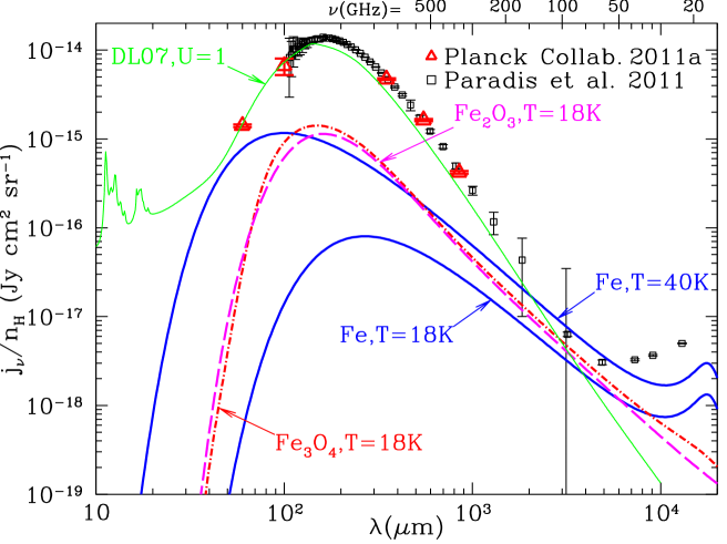
Figure 12: Emission per H calculated if 100% of the interstellar Fe is in $a=0.01\micron$ particles of metallic Fe at $T=18\,{\rm K}$, metallic Fe at $T=40\,{\rm K}$, magnetite Fe₃O₄ at $T=18\,{\rm K}$, maghemite $\gamma$-Fe₂O₃ at $T=18\,{\rm K}$. Also shown are observational determinations of the emission per H from COBE-FIRAS and WMAP (Paradis et al. 2011) (see text) and from IRAS and Planck measurements in the North Ecliptic Pole region (Planck Collaboration et al. 2011a) (see text). Also shown for comparison is emission calculated for the DL07 dust model (Draine & Li 2007) heated by the local starlight radiation field (Mathis et al. 1983). The observed emission from the diffuse ISM does not appear to limit the fraction of Fe that could be in nanoparticles of metallic Fe, magnetite, or maghemite.

Figure 12 shows the predicted emissivity per H nucleon if 100% of the interstellar Fe is in particles of either metallic Fe, magnetite, or maghemite. For the magnetite and maghemite we assume $T\approx 18\,{\rm K}$, characteristic of the bulk of the dust in the diffuse ISM. For metallic Fe, we assume particle size $a\approx 0.01\micron$ (so that eddy currents are not important) and we consider two temperatures: $T\approx 18\,{\rm K}$, appropriate if the metallic Fe is present as inclusions in larger grains, and $T\approx 40\,{\rm K}$, appropriate if the Fe is in free-flying nanoparticles heated by interstellar starlight (see Figure 7).

Figure 12 also shows the mean $110\micron\leq\lambda\leq 1.3\,{\rm cm}$ emission/H measured by COBE-FIRAS and WMAP for regions with $|b|>6^{\circ}$ and $I_{\nu}(240\micron)>18\,{\rm MJy}\,{\rm sr}^{-1}$ (Paradis et al. 2011), as well as the emissivity for low-velocity H I measured by IRAS (60 and 100$\micron$) and Planck (350, 550, and 850$\micron$) around the North Ecliptic Pole (Planck Collaboration et al. 2011a).

From Figure 12 we see that as much as 100% of the Fe could be in single-domain nanoparticles of metallic Fe, magnetite, or maghemite without exceeding the observed emission from the diffuse ISM of the Milky Way.

11.3 Comparison with DL99

Above we have concluded that the observed emission from the ISM does not preclude the bulk of the Fe being in single-domain Fe nanoparticles, whereas DL99 argued that no more than 5% of the Fe was allowed to be in metallic form. These differing conclusions arise from different models used for the magnetic response of Fe at microwave frequencies.

DL99 modeled the magnetic response using a scalar susceptibility $\chi(\omega)$ with the frequency dependence of a damped harmonic oscillator. The resonance frequency $\omega_{0}$ was identified with the precession frequency of spins in the local magnetic field produced by the other spins in the system, and the damping time was set to $\tau_{0}=1/(2\omega_{0})$. This choice of $\tau_{0}$ is probably reasonable for paramagnetic materials, because the local field fluctuates on a time scale related to the precession period of nearby spins. For ferromagnetic or ferrimagnetic materials, however, it is not clear that this damping time is appropriate.

Using this simple damped oscillator form for the magnetic susceptibility, DL99 concluded that nanoparticles of metallic Fe would have a strong absorption peak near 80 GHz, due to the magnetic analogue of a Fröhlich resonance when ${\rm Re}(4\pi\chi)=-3$. Based on observations of dust-correlated emission by the COBE-DMR experiment (Kogut et al. 1996), DL99 argued that no more than $\lesssim 5\%$ of interstellar Fe could be in metallic Fe particles.

The present study employs a more realistic dynamical model for the magnetic response, and reaches a different conclusion. The assumption of a scalar magnetic susceptibility used by DL99 provides a good phenomenological description of paramagnetism or the magnetization of bulk ferromagnetic materials at low frequencies (where the dynamic permeability $\mu(\omega)$ arises from motion of domain walls), but it does not describe the response of magnetic systems at frequencies $\nu\gtrsim 10\,{\rm GHz}$, where precession of the spins is important. The present study uses a tensor susceptibility derived from the Gilbert equation (12). For single-domain Fe particles, the magnetization response (26) has an absorption peak in the 1.5–20 GHz range, depending on shape, and the thermal emission is not as strong as estimated by DL99.

11.4 Validity of the Gilbert Equation

Our model for the magnetic response of Fe, maghemite, and magnetite is based on the Gilbert equation (12), with the dissipation characterized by an adjustable parameter $\alpha_{\rm G}$. We have adopted $\alpha_{\rm G}\approx 0.2$ for purposes of discussion, but the existing experimental literature employs a range of values of $\alpha_{\rm G}$. If the Gilbert equation is used, then $\alpha_{\rm G}\approx 0.2$ gives about the highest values possible for the absorption at $\nu\gtrsim 100\,{\rm GHz}$ (see Figure 5). If $\alpha_{\rm G}$ were to be much smaller (e.g., $\alpha_{\rm G}=0.05$) the opacity would be reduced (by about a factor 3 in going from $\alpha_{\rm G}=0.2$ to $0.05$), and the microwave-submm emissivity would be reduced by the same factor.

Quite aside from the question of what value to use for the Gilbert damping parameter $\alpha_{\rm G}$, we must recognize that the Gilbert equation uses a prescription for the dissipation that is simple and mathematically convenient, but not based on an underlying physical model. Empirical evidence for the accuracy of the Gilbert equation at high frequencies is scant. Laboratory measurements of electromagnetic absorption in Fe and Fe oxide nanoparticles at frequencies up to 500 GHz are required to validate use of the Gilbert equation at these frequencies.

The present treatment of dynamic magnetization assumed that the material was perfectly-ordered and pure, but interstellar grain materials are likely to be non-crystalline and impure. We suspect that lattice defects and impurities will mainly lead to broadening of the resonance appearing near $\omega_{0}$ (for ferromagnetic materials) and $\omega_{\rm res,\pm}$ for ferrimagnetic materials, but this should be studied experimentally. Measurements of the frequency-dependent magnetic polarizability tensor ${\boldsymbol{\alpha}}_{\rm m}(\omega)$ for nanoparticles composed of amorphous Fe-rich oxides or silicates over the frequency range $1-500\,{\rm GHz}$ would be of great value to test the models that have been put forward here.

12 Summary

A substantial fraction of the Fe in the ISM may be in magnetic materials such as metallic iron, magnetite Fe₃O₄, or maghemite $\gamma$-Fe₂O₃. We discuss the implications on the thermal emission from interstellar dust, and the polarization of this emission. The principal conclusions are as follows:

1. We obtain (in Sections 3 and 4) the frequency-dependent magnetic polarizability tensor ${\boldsymbol{\alpha}}_{\rm m}(\omega)$ of single-domain ferromagnetic and ferrimagnetic particles, and evaluate this for three candidate materials: metallic Fe, magnetite Fe₃O₄, and maghemite $\gamma$-Fe₂O₃.

2. Eddy currents are shown to have only a small effect on the magnetic absorption for $\nu\lesssim 500\,{\rm GHz}$.

3. We show (in Section 5) how to calculate the absorption cross section $C_{\rm abs}(\omega)$ for magnetic particles that are small compared to the wavelength.

4. In order to be able to calculate $C_{\rm abs}(\omega)$ we obtain self-consistent dielectric functions for Fe (Appendix B), magnetite (Appendix C), and maghemite (Appendix D), based on a combination of theory and experiment.

5. We confirm the finding of Fischera (2004) for Fe grains that magnetic dipole absorption arising from eddy currents can result in very large absorption cross sections in the FIR and submm for radii $a\gtrsim 0.05\micron$.

6. The Gilbert equation implies that small metallic Fe, magnetite, and maghemite grains have opacities that scale approximately as $\kappa\approx\nu^{0}$ for $10\,{\rm GHz}\lesssim\nu\lesssim 100\,{\rm GHz}$ (see Figs. 5 and 6).

7. We calculate the grain temperature $T$, as a function of radius, for particles of Fe, magnetite, and maghemite heated by starlight (Fig. 7). Small ($a\lesssim 0.03\micron$) Fe grains have $T\approx 40U^{0.2}\,{\rm K}$.

8. If the Gilbert equation with $\alpha_{\rm G}\approx 0.2$ applies at the $\sim$$20\,{\rm kHz}$ rotational frequencies of $\sim 0.1\micron$ grains, then Davis-Greenstein alignment should take place on $\sim$$10^{5}\,{\rm yr}$ time scales, as estimated for ordinary paramagnetic dissipation (Jones & Spitzer 1967). However, it is possible that the Gilbert equation with $\alpha_{\rm G}\approx 0.2$ may significantly underestimate magnetic dissipation at the rotation frequencies of grains, in which case grains with a significant fraction of the volume contributed by ferromagnetic or ferrimagnetic material may undergo rapid alignment by the Davis-Greenstein mechanism.

9. We calculate the expected polarization of the magnetic dipole emission from aligned free-flying magnetic nanoparticles. The polarization has the “normal” sense (${\bf E}\perp{\bf B}_{\rm ISM}$) and can be large (see Figure 9).

10. We calculate the expected polarization of the emission from a nonspherical silicate host with randomly-oriented magnetic inclusions. The magnetic dipole emission becomes important at low frequencies, and can result in a reversal of the polarization direction (see Figure 10).

11. We show (Fig. 12) that up to 100% of interstellar Fe could be in grains of metallic Fe, magnetite, and maghemite without exceeding the observed emission from interstellar dust at frequencies $\nu>30\,{\rm GHz}$.

Appendix A Bloch-Bloembergen Equation

Let ${\bf M}(t)$ be the magnetization. Equations for $d{\bf M}/dt$ all include a term $-\gamma{\bf M}\times{\bf H}_{T}$ for the torque arising from applied field and crystalline anisotropies. This torque is clearly nondissipative, and additional terms must be added to represent the effects of dissipation.

Many studies of paramagnetic resonance employ the Bloch-Bloembergen equation (Bloch 1946; Bloembergen 1950):

$$\left(\frac{d{\bf M}}{dt}\right)_{\rm BB}=\gamma{\bf M}\times{\bf H}_{T}-\frac{{\bf M}_{\parallel}-{\bf M}_{0}}{\tau_{1}}-\frac{{\bf M}_{\perp}}{\tau_{2}}~{}~{}~{},$$ (A1)

where ${\bf M}_{\parallel}\equiv({\bf M}\cdot{\bf M}_{0}){\bf M}_{0}/|M_{0}|^{2}$, and ${\bf M}_{\perp}\equiv{\bf M}-{\bf M}_{\parallel}$ are the components of the magnetization parallel and perpendicular to the stationary magnetization ${\bf M}_{0}$ that would be present if the oscillating field ${\bf h}_{0}$ were set to zero and the magnetization were allowed to reach equilibrium. The time $\tau_{1}$ is interpreted as the spin-lattice relaxation time, the time required for the spin system to exchange heat with the lattice. The time $\tau_{2}$ is interpreted as the spin-spin relaxation time, the time for one spin to be perturbed by nearby spins. The Bloch-Bloembergen equation appears on the surface to be reasonable, and is frequently used. Here we show that this equation is unphysical.

Consider a weak periodic driving field of the form (9). Linearizing, we obtain

$$-i\omega m_{0x} = ~{}\gamma m_{0y}\left[H_{0}+H_{Kz}-D_{zz}M_{0}\right]-\gamma M_{0}\left[h_{0y}-D_{yy}m_{0y}\right]-m_{0x}\tau_{2}^{-1}$$ (A2)

$$-i\omega m_{0y} = \!\!-\gamma m_{0x}\left[H_{0}+H_{Kz}-D_{zz}M_{0}\right]+\gamma M_{0}\left[h_{0x}-D_{xx}m_{0x}\right]-m_{0y}\tau_{2}^{-1}~{}~{}~{}.$$ (A3)

To simplify, assume the sample to be a spheroid, with $D_{yy}=D_{xx}$. With the definitions of $\omega_{0}$ and $\omega_{M}$ from (19, 21) and

$$q\equiv\omega\left(1-\frac{1}{i\omega\tau_{2}}\right)~{}~{}~{},$$ (A4)

the oscillating magnetization ${\bf m}_{0}$ obeys the tensor equation (27), but with

$$\chi_{\pm}^{\rm BB}\equiv\frac{(\omega_{0}\pm q)\omega_{M}}{\omega_{0}^{2}-q^{2}}=\frac{\omega_{M}}{\omega_{0}\mp q}~{}~{}~{}.$$ (A5)

As before, the eigenvectors are the two circular polarizations (28), with the magnetization given by (29). For the two circular polarizations, the magnetization response is given by $\chi_{+}$ and $\chi_{-}$.

Dissipation is given by ${\rm Im}(\chi)$: straighforward algebra yields

$${\rm Im}(\chi_{\pm}^{\rm BB})=\frac{\pm~{}\omega_{M}\tau_{2}^{-1}}{(\omega_{0}\mp\omega)^{2}+\tau_{2}^{-2}}~{}~{}~{}.$$ (A6)

Thus, for anticlockwise circular polarization $\hat{\bf h}_{+}$, the Bloch-Bloembergen equation has positive dissipation (${\rm Im}(\chi_{+})>0$). However, for the clockwise circular polarization $\hat{\bf h}_{-}$, (A6) has ${\rm Im}(\chi_{-})<0$: the dissipation is negative, which is clearly unphysical. The Bloch-Bloembergen equation is frequently applied to studies of magnetic resonance. This unphysical aspect of the Bloch-Bloembergen equation has been previously noted (Lax & Button 1962; Berger et al. 2000), it is surprising that it does not appear to be widely recognized.

The Gilbert equation (12) was proposed by (Gilbert 1955, 2004) as a simple way of including dissipation in the dynamics of ferromagnetic resonance. If we try to require these to have similar response functions $\chi_{\pm}$ for some frequency $\omega$, we would have

$$\chi_{\pm}^{\rm G}(\omega)\approx\chi_{\pm}^{\rm BB}(\omega)~{}~{}~{}.$$ (A7)

Comparison of (26) and (A5) implies that we would need to have

$$\alpha_{\rm G}\omega\approx\pm\tau_{2}^{-1}~{}~{}~{}.$$ (A8)

Clearly this cannot be satisfied simultaneously for both circular polarization modes. If we limit consideration to the $\hat{\bf h}_{+}$ circular polarization mode, we would have $\alpha_{\rm G}\omega\approx\tau_{2}^{-1}$: the assumption of constant $\alpha_{\rm G}$ corresponds to a Bloch-Bloembergen spin-spin relaxation time $\tau_{2}\propto\omega^{-1}$. In other words, the Gilbert equation implies that for high driving frequencies $\omega$ the relaxation time is shorter than for low driving frequencies. This would presumably arise from a spectrum of relaxation processes with a broad range of characteristic time scales, with the “effective” time scale for a given driving frequency $\omega$ scaling as $1/\omega$.

As seen above, the Bloch-Bloembergen equation (A1) is unphysical, implying negative dissipation for the $\hat{\bf h}_{-}$ circular polarization. Whether the phenomenological representation of dissipation in the Gilbert equation provides a good approximation to real materials is a question that can only be answered experimentally. We have not been able to find experimental data that provide a convincing answer.

Appendix B Dielectric Function and Conductivity of Metallic Fe

To calculate emission and absorption by Fe grains, we require the complex dielectric function $\epsilon(\omega)$ and complex magnetic permeability ${\boldsymbol{\mu}}(\omega)$. Because we need to calculate heating of the grain by starlight as well as thermal emission, we require the dielectric function from the ultraviolet to microwave. We undertake to construct the complete dielectric function from microwave to X-rays.

Fe is body-centered cubic, and the dielectric function is a scalar $\epsilon=\epsilon_{1}+i\epsilon_{2}$, if magneto-optical effects are ignored. The real part $\epsilon_{1}$ will be obtained from the imaginary part $\epsilon_{2}$ using the Kramers-Kronig relation (Landau et al. 1993)

$$\epsilon_{1}(\omega)=1+\frac{2}{\pi}P\int_{0}^{\infty}\frac{x\epsilon_{2}(x)}{x^{2}-\omega^{2}}dx~{}~{}~{},~{}~{}~{}$$ (B1)

where $P$ indicates that the principal value is to be taken.

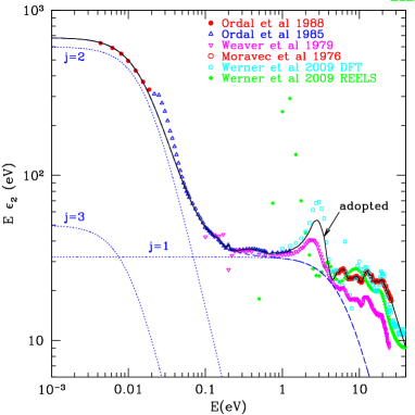
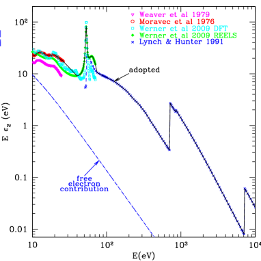
Figure 13: $\hbar\omega\epsilon_{2}(\omega)$ for metallic Fe from Moravec et al. (1976), Weaver et al. (1979), Ordal et al. (1985, 1988), Lynch & Hunter (1991), and Werner et al. (2009). The solid curve shows $\hbar\omega\epsilon_{2}(\omega)$ adopted for this study. The dotted curves show the three free-electron contributions that together (dashed curve) reproduce the adopted $\hbar\omega\epsilon_{2}(\omega)$ at low energies.

Figure 13 shows various determinations of $\epsilon_{2}$ for bulk Fe. When different determinations of $\epsilon_{2}$ in the optical and vacuum ultraviolet region disagree, we have tried to follow the data that appear to be most reliable. In the 1.24–4.75 eV range we take the mean of the experimental results of Weaver et al. (1979) and the density functional theory (DFT) estimates of Werner et al. (2009). In the 5–26 eV range we adopt the values of Moravec et al. (1976). From 45–70.5 eV we take the reflection energy loss spectroscopy (REELS) results from Werner et al. (2009). Above 75 eV we use $\epsilon_{2}$ calculated by Lynch & Hunter (1991) using parameters from Henke et al. (1988).

Table 4: Free-electron model parameters for bulk Fe at $T=293\,{\rm K}$

$j$	$\hbar\tau_{b,j}^{-1}$	$\hbar\omega_{p,j}^{2}\tau_{b,j}$	$\hbar\omega_{p,j}$	$\tau_{b,j}$	$v_{F}\tau_{b,j}$
	(eV)	(eV)	(eV)	(s)	(cm)
1	6.5	32	14.4	$1.01\times 10^{-16}$	$2.00\times 10^{-8}$
2	0.0165	600	3.146	$3.99\times 10^{-14}$	$7.90\times 10^{-6}$
3	0.010	50	0.707	$6.59\times 10^{-14}$	$1.30\times 10^{-5}$

The optical properties of bulk Fe has been measured over a wide range of frequencies (Lynch & Hunter 1991). The dielectric function can be separated into contributions from free electrons and bound electrons:

$$\epsilon(\omega)=1+\delta\epsilon^{\rm(f)}(\omega)+\delta\epsilon^{\rm(b)}(\omega)~{}~{}~{}.$$ (B2)

The free-electron contribution can be approximated by a sum of three Drude free-electron components

$$\delta\epsilon^{\rm(f)}(\omega)=i\sum_{j=1}^{3}\frac{\omega_{p,j}^{2}\tau_{j}}{\omega(1-i\omega\tau_{j})}~{}~{}~{}.$$ (B3)

The free-electron contribution is taken to be large enough that ${\rm Im}(\delta\epsilon^{\rm(b)})\rightarrow 0$ as $\omega\rightarrow 0$. The conductivity from the free-electron component is

$$\sigma(\omega) = \frac{1}{4\pi}\omega\epsilon_{2}(\omega)$$ (B4)

$$= \frac{1}{4\pi}\sum_{j}\frac{\omega_{p,j}^{2}\tau_{b,j}}{1+(\omega\tau_{j})^{2}}~{}.$$ (B5)

Taking $\tau_{j}$ to be the bulk values $\tau_{b,j}$ in Table 4, we obtain a zero-frequency conductivity $\sigma(0)=8.24\times 10^{16}\,{\rm s}^{-1}$, in good agreement with the measured room temperature value $\sigma(0)=9.12\times 10^{16}\,{\rm s}^{-1}$ (Ho et al. 1983).

The bound-electron contribution $\delta\epsilon_{2}^{\rm(b)}(\omega)$ is taken to be the difference $\epsilon_{2}(\omega)-\delta\epsilon_{2}^{\rm(f)}(\omega)$. Because $\epsilon_{2}$ is dominated by $\delta\epsilon_{2}^{\rm(f)}$ at low frequencies, the low-frequency behavior of $\delta\epsilon_{2}^{\rm(b)}$ is unimportant. For mathematical convenience, we assume $\delta\epsilon_{2}^{\rm(b)}\propto\omega$ for $h\nu\lesssim 0.3\,{\rm eV}$.

Figure 14: Real and imaginary components of the bound-electron contribution $\delta\epsilon^{(b)}(\omega)$ to the dielectric function of Fe.

B.1 Temperature Dependence and Effects of Impurities

Fischera (2004) noted that the strong $T$ dependence of the electrical conductivity $\sigma(\omega)$ of bulk Fe implies strong $T$ dependence of the absorption cross section in the FIR. The bulk electrical conductivity $\sigma(0)$ of pure Fe increases by a factor 335 (from $9.2\times 10^{16}\,{\rm s}^{-1}$ to $3.1\times 10^{19}\,{\rm s}^{-1}$) as $T$ is reduced from $293\,{\rm K}$ to $20\,{\rm K}$ (Ho et al. 1983). Thermal contraction causes the $\omega_{p,j}^{2}$ to increase by only about 0.2%, and therefore the large increase in $\sigma(0)$ is almost entirely due to a decrease in the scattering rates $\tau_{j}^{-1}$. Pure Ni shows a similar increase in conductivity with decreasing $T$.

The solar ratio of Fe:Ni is 95:5. If Fe grains exist in the ISM, it seems likely that they will contain appreciable amounts of Ni. Even a few % of Ni alloyed with Fe strongly limits the rise in electrical electrical conductivity at low temperatures: 1% Ni by mass limits the $T=20\,{\rm K}$ conductivity to $4.7\times 10^{17}\,{\rm s}^{-1}$, and 5% Ni limits it to $1.1\times 10^{17}\,{\rm s}^{-1}$ (Ho et al. 1983). The $T=20\,{\rm K}$ conductivity of a Fe:Ne::95:5 alloy is only $2.4$ times larger than the $T=293\,{\rm K}$ value, and is similar to the $T=293\,{\rm K}$ conductivity of pure Fe.

In view of the likely importance of impurity scattering, we will neglect $T$-dependence of the electrical conductivity and $\epsilon(\omega)$, and we will use the room-temperature properties of pure Fe as a reasonable approximation to the properties of interstellar Fe:Ni particles at low ($10$ – $50\,{\rm K}$) temperatures.

B.2 Small Particle Effects

The Fermi velocity in Fe is $v_{\rm F}=1.98\times 10^{8}\,{\rm cm}\,{\rm s}^{-1}$ (Ashcroft & Mermin 1976). For Drude components 2 and 3 (see Table 4), the electron mean free path $v_{\rm F}\tau_{j}$ may be comparable to or larger than the grain size, and therefore the dielectric function must be modified to allow for electron scattering at the grain surface. To allow for this, we follow previous workers (Draine & Lee 1984; Fischera 2004) and set

$$\tau_{j}^{-1}=\tau_{b,j}^{-1}+\frac{v_{\rm F}}{a}~{}~{}~{}.$$ (B6)

This modification of the free-electron contribution to the dielectric function has no noticeable effect at optical frequencies or higher, but, because of the relatively long mean free path $v_{\rm F}\tau_{b,j}$ for free-electron components $j=2$ and $3$ (see Table 4), electron scattering from the grain surface can affect the far-infrared (FIR) absorption when the particle size drops below $\sim 1\micron$.

Appendix C Dielectric Function and Conductivity of Magnetite Fe₃O₄

Unfortunately, there does not appear to be a published dielectric function for magnetite extending from the far-infrared to the far-UV. In the infrared, there are often large disagreements between different studies. Here we attempt to synthesize a complete dielectric function for magnetite from microwave to X-ray frequencies.

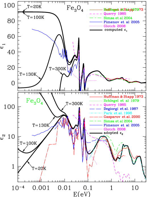
Figure 15: Lower: solid line $=\epsilon_{2}(\omega)$ for bulk magnetite at $T=300\,{\rm K}$, $130\,{\rm K}$, $100\,{\rm K}$, and $20\,{\rm K}$ (see text) together with $\epsilon_{2}$ from Huffman & Stapp (1973), Schlegel et al. (1979), Querry (1985), Degiorgi et al. (1987), Park et al. (1998), Gasparov et al. (2000), Šimša et al. (2002), Pimenov et al. (2005), and Glotch (2008). For $T<80\,{\rm K}$, the contribution of free electrons is negligible. Upper: solid line $=\epsilon_{1}(\omega)$ obtained from $\epsilon_{2}$ using the Kramers-Kronig relation (B1), together with values from the literature.

At room temperature, magnetite is a conductor, with d.c. conductivity $\sigma_{\rm dc}\approx 250\,{\rm ohm}^{-1}\,{\rm cm}^{-1}$$=2.3\times 10^{14}\,{\rm s}^{-1}$, but $\sigma_{\rm dc}$ decreases abruptly, by a factor $\sim$$10^{2}$, upon cooling through the Verwey transition temperature $T_{V}=119\,{\rm K}$. At lower temperatures it behaves like a semiconductor. For high-quality samples, the d.c. conductivity is

$$\sigma_{\rm dc} \approx \left(3\times 10^{16}e^{-1330\,{\rm K}/T}+3\times 10^{12}e^{-740\,{\rm K}/T}\right)\,{\rm s}^{-1}\hskip 10.00002pt{\rm for~{}}45\,{\rm K}<T<T_{V}$$ (C1)

$$\approx 2.3\times 10^{14}\,{\rm s}^{-1}\left(\frac{T-100\,{\rm K}}{160\,{\rm K}}\right)\hskip 80.00012pt{\rm for~{}}T_{V}<T\lesssim 260\,{\rm K}$$ (C2)

$$\approx 2.3\times 10^{14}\,{\rm s}^{-1}\hskip 144.00015pt{\rm for~{}}260\,{\rm K}<T<450\,{\rm K}$$ (C3)

(Miles et al. 1957; Degiorgi et al. 1987; Tsuda et al. 1991). Thus $\sigma_{\rm dc}\lesssim 3\times 10^{4}\,{\rm s}^{-1}$ at the $T\leq 40\,{\rm K}$ temperatures of interstellar grains.

The “free-electron” contribution to the dielectric function is (see eq. B3)

$$\delta\epsilon^{\rm(f)}=\frac{4\pi i\sigma_{\rm dc}}{\omega}\times\frac{1}{(1-i\omega\tau)}~{}~{}~{},$$ (C4)

where $\tau$ is the mean-free-time between scatterings by phonons, impurities, or boundaries. Degiorgi et al. (1987) estimated $\tau_{\rm bulk}=3.1\times 10^{-13}\,{\rm s}$ at $T=130\,{\rm K}$; we use this value for $T<130\,{\rm K}$. For a Fermi speed $v_{\rm F}\approx 10^{8}\,{\rm cm}\,{\rm s}^{-1}$ this corresponds to a mean-free-path $v_{\rm F}\tau_{\rm bulk}\approx 3\times 10^{-5}\,{\rm cm}$. For nanoparticles we take

$$\tau^{-1} = \tau_{\rm bulk}^{-1}+\frac{v_{\rm F}}{a}$$ (C5)

$$\delta\epsilon^{\rm(f)} = \frac{4\pi i\sigma_{\rm dc}\tau}{\omega\tau_{\rm bulk}}\times\frac{1}{1-i\omega\tau}$$ (C6)

At room temperature $\sigma_{\rm dc}$ is large enough that $\delta\epsilon^{\rm(f)}$ makes a significant contribution to $\epsilon(\omega)$ for $\omega<10^{14}\,{\rm s}^{-1}$. For $T<40\,{\rm K}$, $\sigma_{\rm dc}$ is small enough that $\delta\epsilon^{\rm(f)}$ can be neglected for $\omega/2\pi\gtrsim 1\,{\rm GHz}$.

Table 5: Resonance parameters for Fe₃O₄

$j$	$\hbar\omega_{j}(\,{\rm eV})$	$\lambda_{j}(\micron)$	$\gamma_{j}$	$S_{j}$	ref
1	0.0115	108.	1.226	54.9	Degiorgi et al. (1987)
2	0.0315	39.	0.448	7.51	Degiorgi et al. (1987)
3	0.0425	29.	0.0965	8.47	Degiorgi et al. (1987)
4	0.068	18.	0.1162	4.20	Degiorgi et al. (1987)
5	0.35	3.5	0.60	2.0	this work
6	0.60	2.1	1.00	8.5	this work
7	1.9	0.65	0.35	0.30	this work
8	3.2	0.39	0.25	0.90	this work
9	4.0	0.31	0.25	0.45	this work
10	5.0	0.25	0.42	1.60	this work
11	7.0	0.177	0.28	0.21	this work
12	13.	0.095	0.47	0.55	this work
13	17.	0.073	0.40	0.60	this work

Guided by available data (shown in Figure 15) we adopt the function $\epsilon_{2}(\omega)$ shown in Figure 15. At optical and infrared frequencies, the dielectric function is approximated by

$$\epsilon(\omega)=1+\Delta\epsilon+\delta\epsilon^{\rm(f)}+\sum_{j=1}^{13}\frac{S_{j}}{1-(\omega/\omega_{j})^{2}-i\gamma_{j}(\omega/\omega_{j})}$$ (C7)

where the $\omega_{j}$, $\gamma_{j}$, and $S_{j}$ are listed in Table 5 and $\Delta\epsilon=0.375$ is the expected contribution to ${\rm Re}(\epsilon)$ from absorption at $h\nu\gtrsim 30\,{\rm eV}$. Resonance parameters for $j\leq 4$ are taken from the $T=130\,{\rm K}$ results of Degiorgi et al. (1987). Adding resonances $5\leq j\leq 13$ generates a dielectric function that is consistent with a subset of the data in Figure 15.

For $h\nu>30\,{\rm eV}$ we estimate $\epsilon_{2}$ from the sum of the absorption cross sections for 3 neutral Fe atoms and 4 neutral O atoms. Our adopted $\epsilon_{2}(\omega)$, together with the various experimental determinations, are shown in Figure 15. We calculate the real part $\epsilon_{1}$ from our adopted $\epsilon_{2}(\omega)$ using the Kramers-Kronig relation (B1). The resulting $\epsilon_{1}$ is shown in Fig. 15.

Tikhonov et al. (2010) measured the 12–145$\,{\rm GHz}$ dielectric function of magnetite at $T\approx 300\,{\rm K}$. At 140$\,{\rm GHz}$ they found $m\approx 20+0.1i$, or $\epsilon=m^{2}\approx 400+4i$. With the room temperature conductivity $\sigma_{\rm dc}=2.3\times 10^{14}\,{\rm s}^{-1}$ we would expect ${\rm Im}(\epsilon)=4\pi\sigma_{\rm dc}/\omega\approx 3300$ at 140$\,{\rm GHz}$ – almost 3 orders of magnitude larger than the value found by Tikhonov et al. (2010). The results of Tikhonov et al. (2010) are inconsistent with the results of Degiorgi et al. (1987) and Pimenov et al. (2005) but the reason for the discrepancy is unclear.

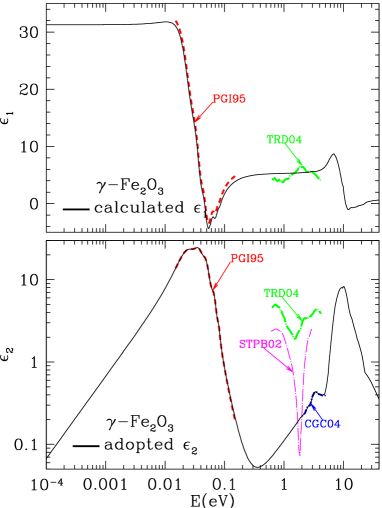
Figure 16: Lower: solid line $=\epsilon_{2}(\omega)$ adopted for maghemite. Upper: solid line $=\epsilon_{1}(\omega)$ derived from the adopted $\epsilon_{2}$. Experimental results (see text): PGI95 (Pecharromán et al. 1995); STPB02 (Šimša et al. 2002); CGC04 (Chakrabarti et al. 2004); TRD04 (Tepper et al. 2004).

Appendix D Dielectric Function of Maghemite $\gamma$-Fe₂O₃

Maghemite ($\gamma$-Fe₂O₃) is considered to be a semiconductor. The band gap is variously estimated to be $E_{g}=2.03\,{\rm eV}$ (Cornell & Schwertmann 2003) and $2.43\,{\rm eV}$ (Chakrabarti et al. 2004). Maghemite has a spinel structure. Each unit cell contains vacancies that may or may not have long-range order. If the vacancies are located randomly, the material is said to have $Fd\bar{3}m$ symmetry. The infrared dielectric function of $Fd\bar{3}m$ $\gamma$-Fe₂O₃ has been determined by Pecharromán et al. (1995) from 0.015 – $0.15\,{\rm eV}$ reflectivity measurements. Pecharromán et al. (1995) fit the IR behavior with 5 damped oscillators.

Chakrabarti et al. (2004) have measured the absorption coefficient $\alpha(h\nu)$ in $\gamma$-Fe₂O₃ films over the range $1.95<h\nu/{\rm eV}<4.95$. For $1.95<(h\nu/\,{\rm eV})<2.5$, the measured absorption coefficient greatly exceeded that expected for a semiconductor with a $2.43\,{\rm eV}$ bandgap.

We obtain $\epsilon_{2}$ from the measured $\alpha$

$$\epsilon_{2}=2{\rm Re}(m){\rm Im}(m)=\frac{{\rm Re}(m)\alpha\lambda_{\rm vac}}{2\pi}~{}~{}~{},$$ (D1)

where $m$ is the complex refractive index, and ${\rm Re}(m)\approx 2.5$ in the optical (Pecharromán et al. 1995). We assumed the electronic contribution to $\epsilon_{2}\propto h\nu$ for $h\nu<2\,{\rm eV}$. At $h\nu\approx 1\,{\rm eV}$ this extrapolation approximately reproduces the measured absorption in amorphous Fe₂O₃ films (Özer & Tephean 1999).

Tepper et al. (2004) have measured the optical constants of pulsed-laser-deposited iron oxide films between $0.6$ and $4.1\,{\rm eV}$. X-ray diffraction studies indicate the films to consist of polycrystalline $\gamma$-Fe₂O₃, but the measured absorption was 5–10 times stronger than in the “pure $\gamma$-Fe₂O₃” nanoparticles studied by Chakrabarti et al. (2004). Tepper et al. (2004) found the absorption to depend on the deposition conditions, weakening if oxygen is present, and they attribute the strong absorption to an excess of Fe²⁺ ions present in the films. Given the availability of oxygen in the ISM, we will adopt the Chakrabarti et al. (2004) results, but the Tepper et al. (2004) data indicate the large uncertainty concerning the optical absorption properties of $\gamma$-Fe₂O₃ material.

Unfortunately, there do not appear to be published measurements of $\gamma-$Fe₂O₃ above $5\,{\rm eV}$. For $E>25\,{\rm eV}$ we estimate the absorption as the sum of the photoelectric absorption by isolated Fe and O atoms, and obtain $\epsilon_{2}$ from (D1) with ${\rm Re}(m)\approx 1$. For $h\nu>5\,{\rm eV}$ we adopt an entirely ad-hoc $\epsilon_{2}(E)$ that has sufficiently strong absorption in the 5–25$\,{\rm eV}$ range to be consistent with the measured $\epsilon_{1}$ in the visible.

The resulting dielectric function should be reasonably accurate in the infrared and optical, but at vacuum-UV energies ($h\nu>5\,{\rm eV}$) should be regarded as merely illustrative of the expected strong absorption. Figure 16 shows the adopted dielectric function for $\gamma-$Fe₂O₃.

Appendix E Time-Averaged Orientations for a Spinning Grain

Define a Cartesian coordinate system $\hat{\bf x}\hat{\bf y}\hat{\bf z}$ where $\hat{\bf x}$ is the direction to the observer. Let $\Phi$ be the angle between the static magnetic field ${\bf H}_{0}$ and the line of sight. Without loss of generality, assume that ${\bf H}_{0}$ is in the $\hat{\bf x}\hat{\bf y}$ plane:

$${\bf H}_{0}=H_{0}\left(\hat{\bf x}\cos\Phi+\hat{\bf y}\sin\Phi\right)~{}~{}~{}.$$ (E1)

Consider a prolate spheroid, spontaneously magnetized along the long axis. The grain is assumed to be spinning with the long axis perpendicular to the angular momentum ${\bf J}$. The angular momentum ${\bf J}$ will precess around ${\bf H}_{0}$. Let $\psi$ be the angle between ${\bf J}$ and ${\bf H}_{0}$, and let $\zeta$ be a precession angle:

$$\hat{\bf J}=(\hat{\bf x}\cos\Phi+\hat{\bf y}\sin\Phi)\cos\psi+\sin\psi\left[\left(\hat{\bf x}\sin\Phi-\hat{\bf y}\cos\Phi\right)\cos\zeta+\hat{\bf z}\sin\zeta\right]~{}~{}~{}.$$ (E2)

Let $\hat{\bf z}_{\rm m}$ be the direction of magnetization of the grain; the $\hat{\bf x}_{\rm m}$,$\hat{\bf y}_{\rm m}$ directions are perpendicular to the magnetization. Let $\hat{\bf x}_{\rm m}$ be parallel to ${\bf J}$; $\hat{\bf y}_{\rm m}$ and $\hat{\bf z}_{\rm m}$ will spin around ${\bf J}$ with the grain’s angular velocity $\Omega$:

$$\hat{\bf x}_{\rm m} = \left(\cos\Phi\cos\psi+\sin\Phi\sin\psi\cos\zeta\right)\hat{\bf x}+\left(\sin\Phi\cos\psi-\cos\Phi\sin\psi\cos\zeta\right)\hat{\bf y}+\left(\sin\psi\sin\zeta\right)\hat{\bf z}~{}~{}~{}~{}~{}$$ (E3)

$$\hat{\bf y}_{\rm m} = \left[-\sin\Phi\sin\zeta\cos\Omega t+\left(\sin\Phi\cos\psi\cos\zeta-\cos\Phi\sin\psi\right)\sin\Omega t\right]\hat{\bf x}+$$ (E4)

$$\left[\cos\Phi\sin\zeta\cos\Omega t-\left(\cos\Phi\cos\psi\cos\zeta+\sin\Phi\sin\psi\right)\sin\Omega t\right]\hat{\bf y}+$$

$$\left[\cos\zeta\cos\Omega t+\cos\psi\sin\zeta\sin\Omega t\right]\hat{\bf z}$$

$$\hat{\bf z}_{\rm m} = \left[\sin\Phi\sin\zeta\sin\Omega t+\left(\sin\Phi\cos\psi\cos\zeta-\cos\Phi\sin\psi\right)\cos\Omega t\right]\hat{\bf x}+$$ (E5)

$$\left[-\cos\Phi\sin\zeta\sin\Omega t-\left(\cos\Phi\cos\psi\cos\zeta+\sin\Phi\sin\psi\right)\cos\Omega t\right]\hat{\bf y}+$$

$$\left[-\cos\zeta\sin\Omega t+\cos\psi\sin\zeta\cos\Omega t\right]\hat{\bf z}~{}~{}~{}.$$

Thus, noting that $\langle\sin^{2}\zeta\rangle=\langle\cos^{2}\zeta\rangle=\langle\sin^{2}\Omega t\rangle=\langle\cos^{2}\Omega t\rangle=1/2$, we have

$$\langle(\hat{\bf y}\cdot\hat{\bf x}_{\rm m})^{2}\rangle = \sin^{2}\Phi\cos^{2}\psi+\frac{1}{2}\cos^{2}\Phi\sin^{2}\psi$$ (E6)

$$\langle(\hat{\bf y}\cdot\hat{\bf y}_{\rm m})^{2}\rangle=\langle(\hat{\bf y}\cdot\hat{\bf z}_{\rm m})^{2}\rangle = \frac{1}{4}\cos^{2}\Phi(1+\cos^{2}\psi)+\frac{1}{2}\sin^{2}\Phi\sin^{2}\psi$$ (E7)

$$\langle(\hat{\bf z}\cdot\hat{\bf x}_{\rm m})^{2}\rangle = \frac{1}{2}\sin^{2}\psi$$ (E8)

$$\langle(\hat{\bf z}\cdot\hat{\bf y}_{\rm m})^{2}\rangle=\langle(\hat{\bf z}\cdot\hat{\bf z}_{\rm m})^{2}\rangle = \frac{1}{4}\left(1+\cos^{2}\psi\right)~{}~{}~{}.$$ (E9)

Appendix F Effective Medium Theory

Laboratory measurements of absorption in magnetic nanoparticles generally study samples where the particles are dispersed in a nonmagnetic dielectric matrix. Let the matrix have scalar dielectric function $\epsilon_{\rm mat}$ and magnetic permeability $\mu_{\rm mat}=1$. Assume the magnetic nanoparticles to be spherical, with volume filling factor $f_{\rm fill}$, and to be characterized by scalar dielectric function $\epsilon_{\rm m}$ and magnetic polarizability tensor ${\boldsymbol{\alpha}}_{\rm m}$ given by eq. (34).

We wish to approximate the composite medium by a uniform medium with an effective dielectric function $\epsilon_{\rm eff}(\omega)$ and effective permeability $\mu_{\rm eff}(\omega)$. Unfortunately, there is no exact solution to this problem, with various competing suggestions for how to estimate $\epsilon_{\rm eff}$ and $\mu_{\rm eff}$ (see the discussion in Bohren & Huffman 1983). The effective medium formulation due to Maxwell Garnett is often used, with

$$\epsilon_{\rm eff}=\frac{\left(1-f_{\rm fill}\right)\epsilon_{\rm mat}\left(\epsilon_{\rm m}+2\epsilon_{\rm mat}\right)+3f_{\rm fill}\epsilon_{\rm mat}\epsilon_{\rm m}}{\left(1-f_{\rm fill}\right)\left(\epsilon_{\rm m}+2\epsilon_{\rm mat}\right)+3f_{\rm fill}\epsilon_{\rm mat}}~{}~{}~{}.$$ (F1)

To obtain $\mu_{\rm eff}$ we must take into account the magnetic anisotropy of the magnetic nanoparticles. Suppose that the directions of spontaneous magnetization are randomly distributed. In the dipole limit, this is the same as if 1/6 of the particles have their static magnetization ${\bf M}_{0}$ oriented in each of the $\pm\hat{\bf x}$, $\pm\hat{\bf y}$, and $\pm\hat{\bf z}$ directions. Thus we model the system as consisting of a matrix with 6 types of inclusions, $j=1-6$. As in eq. (29), each type of inclusion develops an internal magnetization in response to the field in the matrix ${\bf h}_{\rm mat}$:

$${\bf m}_{j}=\left[\chi_{+}\hat{\bf h}_{j+}\left(\hat{\bf h}_{j+}^{*}\cdot{\bf h}_{\rm mat}\right)+\chi_{-}\hat{\bf h}_{j-}\left(\hat{\bf h}_{j-}^{*}\cdot{\bf h}_{\rm mat}\right)\right]~{}~{}~{},$$ (F2)

where

$$\hat{\bf h}_{1\pm} = (\hat{\bf x}\pm i\hat{\bf y})/\sqrt{2}~{}~{}~{}~{}{\rm for}~{}~{}{\bf M}_{0}=M_{0}\hat{\bf z}$$

$$\hat{\bf h}_{2\pm} = (\hat{\bf y}\pm i\hat{\bf z})/\sqrt{2}~{}~{}~{}~{}{\rm for}~{}~{}{\bf M}_{0}=M_{0}\hat{\bf x}$$

$$\hat{\bf h}_{3\pm} = (\hat{\bf z}\pm i\hat{\bf x})/\sqrt{2}~{}~{}~{}~{}{\rm for}~{}~{}{\bf M}_{0}=M_{0}\hat{\bf y}$$

$$\hat{\bf h}_{4\pm} = (\hat{\bf x}\mp i\hat{\bf y})/\sqrt{2}~{}~{}~{}~{}{\rm for}~{}~{}{\bf M}_{0}=-M_{0}\hat{\bf z}$$

$$\hat{\bf h}_{5\pm} = (\hat{\bf y}\mp i\hat{\bf z})/\sqrt{2}~{}~{}~{}~{}{\rm for}~{}~{}{\bf M}_{0}=-M_{0}\hat{\bf x}$$

$$\hat{\bf h}_{6\pm} = (\hat{\bf z}\mp i\hat{\bf x})/\sqrt{2}~{}~{}~{}~{}{\rm for}~{}~{}{\bf M}_{0}=-M_{0}\hat{\bf y}~{}~{}~{}.$$ (F3)

It is easily shown that

$$\frac{1}{6}\sum_{j=1}^{6}{\bf m}_{j} = \left(\frac{\chi_{+}+\chi_{-}}{3}\right){\bf h}_{\rm mat}~{}~{}~{}.$$ (F4)

The volume-averaged magnetization is

$$\langle{\bf m}\rangle=\frac{f_{\rm fill}}{6}\sum_{j=1}^{6}{\bf m}_{j}=f_{\rm fill}\frac{(\chi_{+}+\chi_{-})}{3}{\bf h}_{\rm mat}~{}~{}~{}.$$ (F5)

The oscillating field within an inclusion of type $j$ is

$${\bf h}_{j}={\bf h}_{\rm mat}-D{\bf m}_{j}~{}~{}~{},$$ (F6)

where $D$ is the demagnetization tensor [see eq. (15)], with $D=4\pi/3$ for spherical inclusions. The volume-averaged oscillating field is

$$\langle{\bf h}\rangle = (1-f_{\rm fill}){\bf h}_{\rm mat}+\frac{f_{\rm fill}}{6}\sum_{j=1}^{6}({\bf h}_{\rm mat}-D{\bf m}_{j})$$ (F7)

$$= \left[1-f_{\rm fill}D\frac{\left(\chi_{+}+\chi_{-}\right)}{3}\right]{\bf h}_{\rm mat}~{}~{}~{}.$$ (F8)

The effective permeability is

$$\mu_{\rm eff}\equiv 1+4\pi\frac{\langle{\bf m}\rangle}{\langle{\bf h}\rangle} = 1+\frac{4\pi f_{\rm fill}(\chi_{+}+\chi_{-})/3}{1-f_{\rm fill}D(\chi_{+}\chi_{-})/3}$$ (F9)

$$= 1+\frac{12\pi f_{\rm fill}(\chi_{+}+\chi_{-})}{9-4\pi f_{\rm fill}(\chi_{+}+\chi_{-})}~{}~{}~{}.$$ (F10)

where eq. (F10) is for spherical inclusions. The effective complex refractive index is $m_{\rm eff}=\sqrt{\epsilon_{\rm eff}\mu_{\rm eff}}$. A wave propagating through the material has an attenuation coefficient

$$\alpha=\frac{2\omega}{c}{\rm Im}\left(\sqrt{\epsilon_{\rm eff}\mu_{\rm eff}}\right)~{}~{}~{}.$$ (F11)

References

- Abe et al. (1976) Abe, K., Miyamoto, Y., & Chikazumi, S. 1976, J. Phys. Soc. Japan, 41, 1894
- Aniano et al. (2012) Aniano, G., Draine, B. T., Calzetti, D., et al. 2012, ApJ, submitted
- Ashcroft & Mermin (1976) Ashcroft, N. W., & Mermin, N. D. 1976, Solid State Physics (New York: Holt, Rinehart and Winston)
- Asplund et al. (2009) Asplund, M., Grevesse, N., Sauval, A. J., & Scott, P. 2009, ARA&A, 47, 481
- Babkin et al. (1984) Babkin, E. V., Koval, K. P., & Pynko, V. G. 1984, Thin Solid Films, 117, 217
- Berger et al. (2000) Berger, R., Bissey, J.-C., & Kliava, J. 2000, J. Phys. Condensed Matter, 12, 9347
- Billas et al. (1993) Billas, I. M. L., Becker, J. A., Châtelain, A., & de Heer, W. A. 1993, Phys. Rev. Lett., 71, 4067
- Bloch (1946) Bloch, F. 1946, Phys. Rev., 70, 460
- Bloembergen (1950) Bloembergen, N. 1950, Phys. Rev., 78, 572
- Bohren & Huffman (1983) Bohren, C. F., & Huffman, D. R. 1983, Absorption and Scattering of Light by Small Particles (New York: Wiley)
- Bot et al. (2010) Bot, C., Ysard, N., Paradis, D., et al. 2010, A&A, 523, A20
- Bushchow (1995) Bushchow, K. H. J., ed. 1995, Progress in Spinel Ferrite Research, ed. K. H. J. Bushchow (Amsterdam: Elsevier)
- Butler & Banerjee (1975) Butler, R. F., & Banerjee, S. K. 1975, J. Geophys. Res., 80, 252
- Cabot et al. (2009) Cabot, A., Alivisatos, A. P., Puntes, V. F., et al. 2009, Phys. Rev. B, 79, 094419
- Chakrabarti et al. (2004) Chakrabarti, S., Ganguli, D., & Chaudhuri, S. 2004, Physica E, 24, 333
- Chlewicki & Laureijs (1988) Chlewicki, G., & Laureijs, R. J. 1988, A&A, 207, L11
- Coey (2010) Coey, J. M. D. 2010, Magnetism and Magnetic Materials (Cambridge: Cambridge Univ. Press)
- Cornell & Schwertmann (2003) Cornell, R. M., & Schwertmann, U. 2003, The Iron Oxides (Weinheim: Wiley-VCH)
- Cox (1990) Cox, P. 1990, A&A, 236, L29
- Davis & Greenstein (1951) Davis, L. J., & Greenstein, J. L. 1951, ApJ, 114, 206
- de Oliveira-Costa et al. (1997) de Oliveira-Costa, A., Kogut, A., Devlin, M. J., et al. 1997, ApJ, 482, L17
- Debye (1909) Debye, P. 1909, Annalen der Physik, 335, 57
- Degiorgi et al. (1987) Degiorgi, L., Wachter, P., & Ihle, D. 1987, Phys. Rev. B, 35, 9259
- Desert et al. (1990) Desert, F.-X., Boulanger, F., & Puget, J. L. 1990, A&A, 237, 215
- Dionne (2006) Dionne, G. F. 2006, J. Appl. Phys., 99, 08M913
- Dionne (2009) Dionne, G. F. 2009, Magnetic Oxides (New York: Springer)
- Draine et al. (2007) Draine, B. T., Dale, D. A., Bendo, G., et al. 2007, ApJ, 663, 866
- Draine & Fraisse (2009) Draine, B. T., & Fraisse, A. A. 2009, ApJ, 696, 1
- Draine & Hensley (2012) Draine, B. T., & Hensley, B. 2012, submitted to ApJ, arXiv:1205.6810
- Draine & Lazarian (1998a) Draine, B. T., & Lazarian, A. 1998a, ApJ, 494, L19
- Draine & Lazarian (1998b) Draine, B. T., & Lazarian, A. 1998b, ApJ, 508, 157
- Draine & Lazarian (1999) Draine, B. T., & Lazarian, A. 1999, ApJ, 512, 740
- Draine & Lee (1984) Draine, B. T., & Lee, H. M. 1984, ApJ, 285, 89
- Draine & Li (2007) Draine, B. T., & Li, A. 2007, ApJ, 657, 810
- Draine & Weingartner (1996) Draine, B. T., & Weingartner, J. C. 1996, ApJ, 470, 551
- Duley (1978) Duley, W. W. 1978, ApJ, 219, L129
- Dutta et al. (2004) Dutta, P., Manivannan, A., Seehra, M. S., Shah, N., & Huffman, G. P. 2004, Phys. Rev. B, 70, 174428
- Fischera (2004) Fischera, J. 2004, A&A, 428, 99
- Fitzpatrick (1999) Fitzpatrick, E. L. 1999, PASP, 111, 63
- Galametz et al. (2009) Galametz, M., Madden, S., Galliano, F., et al. 2009, A&A, 508, 645
- Galametz et al. (2011) Galametz, M., Madden, S. C., Galliano, F., et al. 2011, A&A, 532, A56
- Galliano et al. (2005) Galliano, F., Madden, S. C., Jones, A. P., Wilson, C. D., & Bernard, J.-P. 2005, A&A, 434, 867
- Galliano et al. (2003) Galliano, F., Madden, S. C., Jones, A. P., et al. 2003, A&A, 407, 159
- Gasparov et al. (2000) Gasparov, L. V., Tanner, D. B., Romero, D. B., et al. 2000, Phys. Rev. B, 62, 7939
- Gilbert (1955) Gilbert, T. L. 1955, Phys. Rev., 100, 1243
- Gilbert (2004) Gilbert, T. L. 2004, IEEE Transactions on Magnetics, 40, 3443
- Glotch (2008) Glotch, T. D. 2008, in Lunar and Planetary Inst. Technical Report, Vol. 39, Lunar and Planetary Institute Science Conference Abstracts, 1912
- Goodman & Whittet (1995) Goodman, A. A., & Whittet, D. C. B. 1995, ApJ, 455, L181
- Grossi et al. (2010) Grossi, M., Hunt, L. K., Madden, S., et al. 2010, A&A, 518, L52
- Henke et al. (1988) Henke, B. L., Davis, J. C., Gullikson, E. M., & Perera, R. C. C. 1988, Lawrence Berkeley Laboratory Report No. LBL-26259
- Ho et al. (1983) Ho, C. Y., Ackerman, M. W., Wu, K. Y., et al. 1983, J. Phys. Chem. Ref. Data, 12, 183
- Hoang et al. (2011) Hoang, T., Lazarian, A., & Draine, B. T. 2011, ApJ, 741, 87
- Huffman (1977) Huffman, D. R. 1977, Advances in Physics, 26, 129
- Huffman & Stapp (1973) Huffman, D. R., & Stapp, J. L. 1973, in IAU Symposium, Vol. 52, Interstellar Dust and Related Topics, ed. J. M. Greenberg & H. C. van de Hulst, 297
- Iida (1963) Iida, S. 1963, J. Phys. Chem. Solids, 24, 625
- Israel et al. (2010) Israel, F. P., Wall, W. F., Raban, D., et al. 2010, A&A, 519, A67
- Jenkins (2009) Jenkins, E. B. 2009, ApJ, 700, 1299
- Jones (1990) Jones, A. P. 1990, MNRAS, 245, 331
- Jones & Spitzer (1967) Jones, R. V., & Spitzer, L. J. 1967, ApJ, 147, 943
- Kido et al. (2004) Kido, O., Higashino, Y., Kamitsuji, K., et al. 2004, J. Phys. Soc. Japan, 73, 2014
- Kogut et al. (1996) Kogut, A., Banday, A. J., Bennett, C. L., et al. 1996, ApJ, 464, L5
- Kong et al. (2010) Kong, I., Ahmad, S. H., Abdullah, M. H., et al. 2010, J. Magnetism Magnetic Mat., 322, 3401
- Landau & Lifshitz (1935) Landau, L. D., & Lifshitz, E. M. 1935, Physik Zeitsch. der Sowjet., 8, 153
- Landau et al. (1993) Landau, L. D., Lifshitz, E. M., & Pitaevskii, L. P. 1993, Electrodynamics of Continuous Media (Oxford: Pergamon Press)
- Lax & Button (1962) Lax, B., & Button, K. J. 1962, Microwave Ferrites and Ferrimagnetics (New York: McGraw-Hill)
- Lazarian & Draine (1999) Lazarian, A., & Draine, B. T. 1999, ApJ, 516, L37
- Lazarian & Draine (2000) Lazarian, A., & Draine, B. T. 2000, ApJ, 536, L15
- Leitch et al. (1997) Leitch, E. M., Readhead, A. C. S., Pearson, T. J., & Myers, S. T. 1997, ApJ, 486, L23
- Lynch & Hunter (1991) Lynch, D. W., & Hunter, W. R. 1991, in Handbook of optical constants of solids II, ed. Palik, E. D. (Boston: Academic Press), 385
- Martin (1995) Martin, P. G. 1995, ApJ, 445, L63
- Mathis (1986) Mathis, J. S. 1986, ApJ, 308, 281
- Mathis et al. (1983) Mathis, J. S., Mezger, P. G., & Panagia, N. 1983, A&A, 128, 212
- Mathis et al. (1977) Mathis, J. S., Rumpl, W., & Nordsieck, K. H. 1977, ApJ, 217, 425
- Mie (1908) Mie, G. 1908, Annalen der Physik, 330, 377
- Miles et al. (1957) Miles, P. A., Westphal, W. B., & von Hippel, A. 1957, Rev. Mod. Phys., 29, 279
- Milham (1994) Milham, M. E. 1994, Electromagnetic scattering by magnetic spheres: Theory and algorithms, Technical report
- Moravec et al. (1976) Moravec, T. J., Rife, J. C., & Dexter, R. N. 1976, Phys. Rev. B, 13, 3297
- Morrish (2001) Morrish, A. H. 2001, The Physical Principles of Magnetism (Piscataway, NJ: IEEE Press)
- Neo et al. (2010) Neo, C. P., Yang, Y., & Ding, J. 2010, J. Appl. Phys., 107, 083906
- O’Halloran et al. (2010) O’Halloran, B., Galametz, M., Madden, S. C., et al. 2010, A&A, 518, L58
- Ordal et al. (1985) Ordal, M. A., Bell, R. J., Alexander, R. W., Jr., Long, L. L., & Querry, M. R. 1985, Appl. Opt., 24, 4493
- Ordal et al. (1988) Ordal, M. A., Bell, R. J., Alexander, R. W., Jr., Newquist, L. A., & Querry, M. R. 1988, Appl. Opt., 27, 1203
- Özdemir & Banerjee (1984) Özdemir, Ö., & Banerjee, S. K. 1984, Geophys. Res. Lett., 11, 161
- Özdemir & Dunlop (1999) Özdemir, O., & Dunlop, D. J. 1999, Earth. Plan. Sci. Lett., 165, 229
- Özer & Tephean (1999) Özer, N., & Tephean, F. 1999, Solar Energy Materials and Solar Cells, 56, 141
- Paradis et al. (2011) Paradis, D., Bernard, J. P., Mény, C., & Gromov, V. 2011, A&A, 534, A118
- Park et al. (1998) Park, S. K., Ishikawa, T., & Tokura, Y. 1998, Phys. Rev. B, 58, 3717
- Pecharromán et al. (1995) Pecharromán, C., González-Carreño, T., & Iglesias, J. E. 1995, Phys. Chem. Minerals, 22, 21
- Pimenov et al. (2005) Pimenov, A., Tachos, S., Rudolf, T., et al. 2005, Phys. Rev. B, 72, 035131
- Planck Collaboration et al. (2011a) Planck Collaboration, Abergel, A., Ade, P. A. R., et al. 2011a, A&A, 536, A24
- Planck Collaboration et al. (2011b) Planck Collaboration, Ade, P. A. R., Aghanim, N., et al. 2011b, A&A, 536, A17
- Purcell (1979) Purcell, E. M. 1979, ApJ, 231, 404
- Querry (1985) Querry, M. R. 1985, Optical constants (Contractor Report, Sep. 1982 - May 1984 Missouri Univ., Kansas City), Technical report
- Schalen (1965) Schalen, C. 1965, PASP, 77, 409
- Schlegel et al. (1979) Schlegel, A., Alvarado, S. F., & Wachter, P. 1979, J. Phys. C, 12, 1157
- Shendruk et al. (2007) Shendruk, T. N., Desautels, R. D., Southern, B. W., & van Lierop, J. 2007, Nanotechnology, 18, 455704
- Šimša et al. (2002) Šimša, Z., Thailhades, P., Presmanes, L., & Bonningue, C. 2002, J. Magnetism Magnetic Mat., 242, 381
- Soohoo (1985) Soohoo, R. F. 1985, Microwave magnetics (New York: Harper and Row)
- Tebble & Craik (1969) Tebble, R. S., & Craik, D. J. 1969, Magnetic Materials (London: Wiley-Interscience)
- Tepper et al. (2004) Tepper, T., Ross, C. A., & Dionne, G. F. 2004, IEEE Transactions on Magnetics, 40, 1685
- Tiago et al. (2006) Tiago, M. L., Zhou, Y., Alemany, M. M. G., Saad, Y., & Chelikowsky, J. R. 2006, Phys. Rev. Lett., 97, 147201
- Tikhonov et al. (2010) Tikhonov, V. V., Boyarskii, D. A., Polyakova, O. N., & Goltsman, G. N. 2010, Prog. Electromagnetics Research B, 25, 349
- Tsuda et al. (1991) Tsuda, N., Nasu, K., Yanase, A., & Siratori, K. 1991, Electronic Conduction in Oxides (Berlin: Springer-Verlag)
- Tsuzuki et al. (2011) Tsuzuki, T., Schäffel, F., Muroi, M., & McCormick, P. G. 2011, Journal of Alloys and Compounds, 509, 5420
- Valstyn et al. (1962) Valstyn, E. P., Hanton, J. P., & Morrish, A. H. 1962, Phys. Rev., 128, 2078
- van de Hulst (1957) van de Hulst, H. C. 1957, Light Scattering by Small Particles (New York: John Wiley & Sons)
- Weaver et al. (1979) Weaver, J. H., Colavita, E., Lynch, D. W., & Rosei, R. 1979, Phys. Rev. B, 19, 3850
- Weingartner & Draine (2001) Weingartner, J. C., & Draine, B. T. 2001, ApJ, 548, 296
- Werner et al. (2009) Werner, W. S. M., Glantschnig, K., & Ambrosch-Draxl, C. 2009, J. Phys. Chem. Ref. Data, 38, 1013
- Wickramasinghe & Nandy (1971) Wickramasinghe, N. C., & Nandy, K. 1971, MNRAS, 153, 205
- Wu et al. (2006) Wu, L. Z., Ding, J., Jiang, H. B., et al. 2006, J. Appl. Phys., 99, 083905
- Zubko et al. (2004) Zubko, V., Dwek, E., & Arendt, R. G. 2004, ApJS, 152, 211