Continuous mode cooling and phonon routers for phononic quantum networks
Abstract
We study the implementation of quantum state transfer protocols in phonon networks, where in analogy to optical networks, quantum information is transmitted through propagating phonons in extended mechanical resonator arrays or phonon waveguides. We describe how the problem of a non-vanishing thermal occupation of the phononic quantum channel can be overcome by implementing optomechanical multi- and continuous mode cooling schemes to create a ‘cold’ frequency window for transmitting quantum states. In addition, we discuss the implementation of phonon circulators and switchable phonon routers, which rely on strong coherent optomechanical interactions only, and do not require strong magnetic fields or specific materials. Both techniques can be applied and adapted to various physical implementations, where phonons coupled to spin or charge based qubits are used for on-chip networking applications.
1 Introduction
The successful application of laser cooling techniques for cooling isolated vibrational modes of micro- and nanomechanical devices [1, 2, 3, 4, 5, 6, 7, 8] has recently attracted a lot of interest in the control of macroscopic phononic degrees of freedom on a single quantum level. By now the preparation of mechanical resonators close to the quantum ground state has been achieved in different experimental settings [9, 10, 11] and coherent interfaces between mechanics and other quantum systems like superconducting qubits [9, 12], spins [13, 14] or photons [15, 16] are currently developed. Beyond new possibilities to address fundamental questions in quantum physics [17, 18, 19, 20], these experimental developments also provide the foundation for new, phonon-based quantum technologies. For example, in the context of quantum information processing and quantum communication, optomechanical (OM) slowing of light [21, 22] and first steps towards realizing a mechanical quantum memory [15, 16] have been demonstrated, and the use of mechanical quantum transducers for interfacing different qubit systems [23, 24, 25] has been proposed. For these applications mechanical systems benefit from the ability to interact with a wide range of other electric, magnetic and optical quantum systems, while still maintaining long coherence times and being compatible with scalable nano-fabrication techniques.
The use of phonons for quantum information science applications is not new. Already in the first proposals for quantum computers, it has been suggested to employ vibrational modes of a trapped ion Wigner crystal for transmitting quantum information between spatially separated qubits [26]. More recently it has been shown that these ideas could equally well be applied in systems of coupled macroscopic mechanical resonators [23, 27, 28], which extends the concept of a mechanical quantum bus to a wider range of atomic and solid-state systems. In analogy to optical fields, phonons can be confined in phonon cavities (e.g. represented by a high mechanical resonator), but also propagate freely along phononic waveguides. This suggests that many quantum communication and state-transfer protocols developed in the context of optical quantum networks [29, 30, 31] could – on a smaller physical scale – also be implemented using acoustic phonons. Here, new approaches to design and pattern phonon waveguides based on phononic crystals structures [32, 33] provide a very promising and versatile platform for realizing such phonon networks in practice. However, compared with the relatively advanced field of optical quantum networks [30], many equivalent control techniques still have to be developed for phononic quantum systems, which face the additional challenge that thermal noise in phononic channels is not negligible and would usually by far exceed quantum signals encoded in a single phononic excitation.
In this work we address the problem of implementing quantum communication protocols in thermal phononic channels and show, how the addition of OM control elements can be used to realize a faithful transfer of quantum information between different nodes of the network. As a first key element to achieve this task, we describe the generalization of OM laser cooling techniques to multi- and continuous mode setups. This approach is motivated by a recent proposal for interfacing OM systems (OMS) with phonon waveguides [25], and leads to a strong suppression of thermal noise within the relevant transmission bandwidth. Therefore, instead of pursuing the otherwise challenging task of cooling the whole network, this technique creates a ‘cold’ frequency window, which is sufficient to coherently transfer single quanta through an otherwise ‘hot’ phononic channel.
As a second control tool we describe the implementation of phonon circulators and switchable phonon routers, which enable a directed transfer of propagating phonons through large 1D or 2D networks. In the optical domain circulators or other non-reciprocal devices are usually based on the Faraday-effect. In principle similar effects also exist for acoustic phonons in certain materials [34]. However, due to the required large magnetic fields and the use of materials with non-optimized mechanical properties, this approach is not suited for on-chip phonon quantum networks. Instead, we propose an integrated circulator for acoustic phonons that relies solely on an OM induced non-reciprocity [35, 36], where the directionality is imposed by the phase relation between two optical driving fields. Thereby, the device can be switched on or reversed conveniently and in combination with the above-mentioned cooling techniques, this coherent OM routing scheme is in principle sufficient to fully control the distribution of quantum information in large-scale phonon networks.
The remainder of this paper is structured as follows. In section 2 we first present a brief introduction to phonon networks and the general input-output formalism, which is used to model these systems. In section 3 we revisit OM laser cooling and generalize it to multi- and continuous mode scenarios. As a basic application we then discuss in section 4 how an OM noise filter can be applied to transmit a quantum state through a thermal channel. In section 5 we describe the realization of phonon circulators and routers using coherent OM interactions. Finally, in section 6 we outline several potential systems for implementing phonon networks and then summarize the main results and conclusions of this work in section 7.
2 Phonon quantum networks
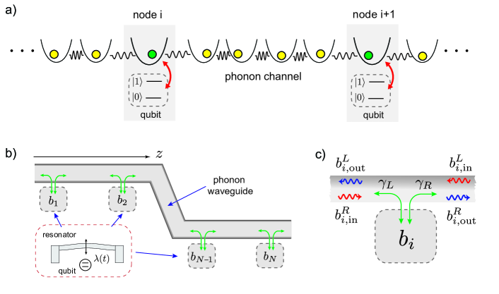
Figure 1a shows a schematic representation of a generic phonon quantum network, where individual nodes are connected via a mechanical quantum bus. In analogy to optical quantum networks, each node contains an isolated solid state two-level system (‘qubit’) with quantum information encoded in states and . The qubits interact with localized phonon modes (‘phonon cavities’), which are in turn weakly coupled to a common set of propagating modes of a phonon waveguide or coupled mechanical resonator array (‘quantum channel’). The full Hamiltonian of this system is given by
| (1) |
where and describe the dynamics of the individual nodes and the phononic channel, respectively, and accounts for the coupling between them. In the following, we assume that the Hamiltonian for the individual nodes takes the form
| (2) |
where the are Pauli operators and the bosonic operators for the local mechanical modes of frequency . The third term describes the coupling between the qubits and the local mechanical modes. For each node the qubit frequency splitting and the qubit-resonator coupling can be tuned independently by changing the qubit frequency or modulating the coupling with local control fields (see section section 6). For this allows for a controlled mapping of the qubit state onto a phonon superposition, which we will use in our discussion of the state transfer below. The implementation of qubit-resonator interactions as given in equation (2) has been described for various charge- and spin-based qubits in the literature and in section 6 we briefly summarize some of the most relevant systems.
2.1 Phonon channels
The mechanical quantum channel which is used to communicate between the nodes can in general be represented by a chain of coupled mechanical resonators,
| (3) |
Here and are the position and momentum operators, is the effective mass, the bare oscillation frequency and the spring constant accounts for the nearest-neighbor coupling. For small the coupled resonators form a discrete set of collective eigenmodes. In this case quantum state transfer and quantum information processing protocols between two qubits can be implemented by addressing only a single collective mode, as has been discussed in the context of trapped ion systems [26] or coupled nanomechanical [23] and optomechanical [28] resonators.
In this work we are primarily interested in the opposite regime of extended arrays, . In this limit can be represented by a dense set of plane wave modes, , where , is the phonon dispersion relation, and, for a lattice spacing , the momentum label is restricted to the first Brillouin zone . This scenario is realized, for example, in large arrays of coupled nanomechanical beams [37] or in phononic band gap structures [32], where each resonator corresponds to a vibrational mode of a unit cell, typically of size m. In the continuum limit we can identify a frequency range away from the band edges in which the coupled resonator array exhibits an approximately linear dispersion , where is the effective speed of sound and a frequency offset. In this case it is convenient to introduce the normalized displacement field , where
| (4) |
describe right- and left-moving mechanical excitations of the phononic channel. Under the assumption of a linear dispersion these fields obey and
| (5) |
By assuming that the frequency of the local mechanical modes also lies within this frequency range, the coupling between the local resonators and the waveguide modes can be approximated by
| (6) |
where is the length of the waveguide and are the positions of the nodes along the waveguide (see figure 1b). Below we identify as the total decay rate of the local resonator modes into the waveguide. Note that equations (5) and (6) are valid for times and distances . An explicit and more detailed derivation of these results is given in A for the case of a simple coupled resonator chain.
2.2 Input- output relations
Under the validity of equations (5) and (6) and in the limit where and the bandwidth are large compared to the other characteristic frequency scales, we can eliminate the waveguide modes and use an input- output formalism [38] to describe the effective dynamics of the coupled nodes. Using (5) and (6) and making a standard Born-Markov approximation, we can derive a set of coupled quantum Langevin equations (QLEs) [38]. For each node we obtain
| (7) |
where is the total decay rate of phonons into the waveguide. For side-coupled phonon cavities we would usually have , but we below we describe scenarios where the emission either to the left or to the right is effectively switched off. In equation (7) we have defined incoming fields (see figure 1c)
| (8) |
which specify the left and right moving waveguide modes before they interact with . Similarly, we introduce the scattered outgoing fields
| (9) |
The dynamics of the whole network is then described by the QLEs (7) together with the input-output-relations at each node,
| (10) |
and the free propagation
| (11) |
where . Under realistic conditions we must also account for intrinsic phonon losses, backscattering and rethermalization, which we address below.
2.3 Optomechanical control techniques for phonon networks
The phonon network described above is formally equivalent to optical quantum networks and can in principle be used in a similar way to transfer quantum states from one node to another [29, 31]. However, in contrast to high frequency optical fields, the thermal population of the phonon modes is usually not negligible. For phonon frequencies in the MHz to GHz regime and temperatures K the number of thermal noise phonons in the waveguide will exceed the quantum signal encoded in a single phonon. In addition, as shown in figure 1c, phonons emitted from a single side-coupled node will naturally propagate along two directions, i.e. . In larger networks or 2D arrangements the inability to route propagating phonons severely limits an efficient implementation of quantum communication protocols.
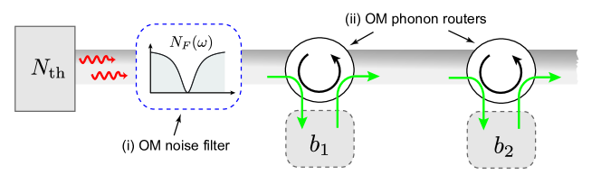
In the remainder of the paper we consider an extended setup as shown in figure 2 and describe how the integration of additional OM control elements can be used to overcome these fundamental limitations of phononic networks. The two key ingredients in this setup are:
-
1.
An OM noise filter, which is used to suppress thermal noise within the relevant transmission bandwidth.
-
2.
Coherent OM phonon circulators or phonon routers, which allow for directed propagation and switchable routing of phonons through the network.
3 Optomechanical noise filters
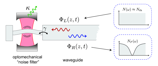
In this section we describe the application of OM laser cooling techniques to suppress thermal noise in an extended phononic quantum channel. Obviously, ground-state cooling of the whole network becomes inefficient as the system size increases, but it is also unnecessary, since usually only a few modes within a small bandwidth are used for transmitting quantum states. In the following we consider a scenario as shown in figure 3, where a single laser-cooled mechanical resonator provides a ‘cold sink’, and within a certain frequency range suppresses the thermal noise of the reflected modes of a continuous waveguide (or the transmitted modes in the case of a side-coupled phonon cavity). A similar configuration has been previously proposed for realizing a traveling-wave photon to phonon converter, where under ‘impedance-matched’ conditions an incoming photon is converted into a traveling phonon and vice versa [25]. In this sense cooling of the waveguide can be interpreted as a mapping of the optical vacuum onto the phonon channel, while in turn mechanical noise is upconverted into optical photons leaving the system.
3.1 Single mode cooling
Before addressing the suppression of thermal noise in extended phonon waveguides, let us first briefly review with the standard scenario for OM cooling [39, 40], where the frequency of an optical cavity mode is modulated by the displacement of a single mechanical mode. The optical cavity is driven by a coherent laser field of frequency and in a frame rotating with the Hamiltonian for the OMS is given by
| (12) |
Here the bosonic operators and represent the optical and the mechanical modes, respectively, is the mechanical oscillation frequency, the OM coupling constant and the strength of the external driving field. Terms rotating with the optical frequency have been neglected by a rotating wave approximation (RWA). The OM interaction, as described by the third term in equation (12), derives from a linear dependence of the optical resonance frequency on the position quadrature of the mechanical mode [41, 42]. Including dissipation through cavity decay and intrinsic mechanical losses, the dynamics of the OMS is described by the QLEs
| (13) | |||||
| (14) |
where is the optical field decay rate and is the mechanical damping rate for an intrinsic mechanical quality factor . The -correlated operators and represent the vacuum input noise of the optical field and the thermal mechanical noise respectively. Within the relevant frequency range the latter is characterized by a non-vanishing equilibrium occupation number .
In the limit of strong driving the external field displaces both the optical and the mechanical modes by a large classical amplitude and , where . For , we can make a unitary transformation and and linearize the OM coupling around the classical mean values,
| (15) |
where we have redefined . If the external driving field is (near) resonant with the red mechanical sideband of the optical cavity, i.e. if , and if we can make a rotating wave approximation (RWA) with respect to and obtain a beam-splitter Hamiltonian
| (16) |
which describes a (near) resonant conversion of phonons into photons (and vice versa). Combined with the decay from the optical cavity, it allows for cooling: incident (noise) phonons are up-converted to photons and decay from the optical cavity.
The QLEs for the linearized OMS can be conveniently solved in the Fourier domain as outlined in more detail in B. In the relevant weak coupling and sideband resolved regime () we then obtain the standard result for the mechanical fluctuation spectrum,
| (17) |
where is the optically induced mechanical damping rate and the reduced steady state resonator occupation number. In the following we are interested in OMS where both and single-mode ground-state cooling can be achieved.
3.2 Optomechanical cooling in a multimode system
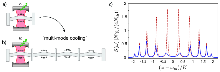
The single mode cooling scheme can be generalized to cool mechanical networks consisting of a few coupled resonators only one of which is OM cooled, as shown in figure 4b. In this case the linearized OM Hamiltonian is given by
| (18) |
where the denote the nearest neighbor couplings and we have already performed a RWA assuming that . The resulting QLEs can be written as
| (19) | |||||
| (20) | |||||
| (21) | |||||
| (22) |
where the are mutually uncorrelated noise operators associated with intrinsic mechanical damping of each mode.
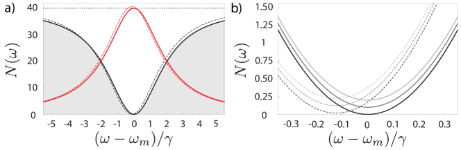
In figure 4c we plot the correlation spectrum for a chain of resonators with assuming that the mode is optically cooled. For reference the dashed line shows the undamped case . In this case the heights of the peaks at frequencies are given by , where are the normalized mode distributions. When the OM coupling is turned on the peaks are broadened and their height is reduced, which corresponds to an overall cooling of the individual eigenmodes. However, we see that cooling occurs in a highly non-uniform way and only the few modes close to the cavity resonance are cooled efficiently. While the details depend on the ratios between , and , we find that this behavior is quite generic and a precursor to the features we identify in the following for the continuous waveguide limit.
3.3 Optomechanical cooling of a mode continuum
Starting from the multi-mode setting shown in figure 4b, let us now address the limit of a continuous mode waveguide as depicted in figure 3 by retaining the OM coupling to the first mode , but describing the other phonon modes in terms of continuous left- and right-propagating fields . If , we can adapt the input-output formalism introduced in section 2 to model the coupling between the localized mode and the rest of the waveguide in terms of the scattering relation
| (23) |
Here and are the incident and reflected waveguide fields and is the characteristic phonon decay rate into the waveguide. Ignoring other, intrinsic loss channels for the moment, we obtain
| (24) | |||||
| (25) |
for the linearized OM dynamics of the local mode and we see that the problem of cooling a continuous waveguide is formally identical to the single-mode cooling considered above. However, instead of looking at the occupation of the local mode we are now interested in the spectrum of the reflected waveguide field , given a thermal incident field . To do so, we solve the QLEs in Fourier space and write the result as
| (26) |
where with “in”, “out”. The matrix is a scattering matrix and a more detailed derivation of equation (26) is given in B. For given input noise correlations we obtain the output correlation matrix .
3.3.1 Optomechanical noise filters.
The quantity that we are interested in is the filtered noise spectrum of the reflected field, which is defined by
| (27) |
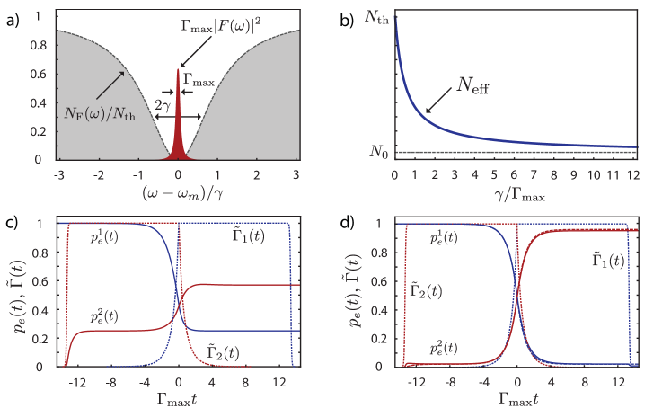
Figure 5a shows the typical frequency dependence of . As expected, we see a strong suppression of thermal noise around the mechanical frequency . For and under the condition , the dynamics of the OMS is well approximated by the beam-splitter Hamiltonian (16) and we obtain
| (28) |
We see that, under these approximations, the ‘impedance matching’ condition [25] results in a complete cancellation of the reflected noise on resonance. In this case the optical decay rate matches the mechanical waveguide coupling and the OMS acts effectively as a double-sided phonon cavity with the thermal mechanical bath on one side and the optical bath on the other side.
Under realistic conditions the noise cancellation described by equation (28) will not be perfect and to account for various imperfections in the system we assume in our discussion below a spectrum of the form
| (29) |
where and now include small corrections of the width and the center of the dip and is a non-vanishing noise floor. Intrinsic limitations that lead to a finite are already contained in the full OM interaction itself, where for any finite off-resonant Stokes-scattering terms in the linearized Hamiltonian (15) induce corrections to the ideal beam-splitter interaction. However, as shown in figure 5b, by accounting for these effects up to second order in we only obtain a small shift of the spectral dip and an offset , which is negligible under the weak coupling conditions mentioned above. A more crucial limitation for the OM noise filter arises from intrinsic mechanical losses of the localized mechanical mode, which can be accounted for by introducing an additional decay rate and associated noise operator in the QLE (25) (see B). This leads to a finite . This means that, while for the optimized case with the local mode can be highly excited, also the condition must be fulfilled to achieve good noise filtering.
3.3.2 Propagation losses and scattering.
The spectrum determines the mechanical noise of the outgoing displacement field immediately after the OM device and for an ideal phonon waveguide this noise spectrum will be the same at all positions . However, in a realistic setting, scattering losses in the waveguide and the associated noise lead to a rethermalization of the noise spectrum and . For an approximately linear dispersion relation the propagation of the outgoing field can be modeled by
| (30) |
where is the phonon mean free path in the waveguide and is a thermal noise field with . In A.1 we outline a microscopic derivation of this result for a coupled mechanical resonator array, where can be connected to the intrinsic damping rate of the individual resonators in the array. For and in a frame rotating with we obtain
and from this result we can derive the full noise spectrum along the waveguide
| (32) |
This result describes the rethermalization of the noise dip on a length scale given by the phonon mean free path. For the relevant distances the noise spectrum can still be described by the Lorentzian shape given in equation (29), but the noise floor increases linearly with the distance to the OM noise filter. Note that similar quantitative conclusions follow from the standard approach of treating propagation losses in terms of a series of beam splitters [25, 38], but the present analysis also provides a direct connection to the underlying microscopic phonon scattering mechanism.
To the extend that the scatterers are linear, phonon backscattering gives rise to small overall losses, which are on equal footing with the thermalization discussed above.
4 Quantum state transfer in a thermal phonon network
We now return to our original goal of implementing a quantum state transfer protocol between two qubits via an extended and thermally occupied phononic channel. For a simplified discussion we consider in the following the state transfer between two nodes assuming a unidirectional coupling, where , and as shown in figure 2. In section 5 below, we describe how this condition can be realized using phonon routers.
4.1 A tunable qubit network
As a first step we describe the implementation of an effective qubit network with tunable qubit-waveguide couplings by eliminating the dynamics of the local phonon modes. We start from the full set of QLEs, which, for each node , derive from the Hamiltonian in (2) and are given by
| (33) | |||||
| (34) | |||||
| (35) |
The input-output relations are
| (36) |
where describes the incident waveguide field before interacting with the first node. Hereafter, we absorb the retardation time by redefining time-shifted operators and control fields for the second node [38] and for simplicity we focus on the resonant case in which .
We are interested in the regime in which the decay of the the local phonon modes into the waveguide is fast compared to the coupling . This allows us to adiabatically eliminate the phonon modes and to derive an effective description in terms of the qubit degrees of freedom only. In the frame rotating with and to lowest order in , (35) can be solved to give
| (37) |
After reinserting this expression into equations (33) and (34) we obtain
| (38) | |||||
| (39) |
Here are tunable qubit decay rates and
| (40) |
the associated effective noise operators which on the timescale obey . Provided that and also vary slowly on this time scale, we find that
| (41) |
Thus we obtain a new set of effective quantum network equations for the qubit operators with tunable decay rates . We emphasize that while in the following this effective description allows a simplified discussion of the state transfer protocol, it is not necessary to consider the regime and a perfect state transfer can also be achieved using the full model [29].
4.2 Quantum state transfer through a phonon channel
Our goal is to implement a quantum state transfer between the two qubits, i.e.
| (42) |
which is achieved via coherent emission and reabsorption of a single phonon in the waveguide. A solution to this problem has been first described for optical networks [29], where it has been shown that by identifying appropriate pulses , a perfect quantum state transfer can be implemented. Let us briefly summarize the main idea behind this scheme, for the moment assuming zero temperature. In this case the waveguide is initially in the vacuum state and the dynamics of the whole system can be restricted to the zero- and one-excitation subspace. Then, for an initial two qubit state , we can define the amplitudes . From the QLEs (38) and (39) and the input-output relation (41), it follows that these amplitudes evolve according to
| (43) | |||||
| (44) |
and for initial amplitudes , the general solutions is given by
| (45) | |||||
| (46) |
Here and
| (47) |
is the state-transfer amplitude. For the initial state given in equation (42), and therefore a perfect transfer is achieved if at some final time the amplitudes approach
| (48) |
While the first condition is easily fulfilled for sufficiently long, but otherwise arbitrary pulses, satisfying the second one requires control over their shape. Perfect state transfer is only possible if the total number of excitations is conserved, i.e., if no population gets lost from the one-excitation subspace. This means that the norm for all times, which after taking the time-derivative of this condition yields
| (49) |
This result also follows from the requirement that the total scattered field after the second node vanishes at all times, i.e. . Therefore equation (49) is often referred to as the dark-state condition.
A set of pulses and that realize a perfect state transfer can always be found numerically by choosing such that and then solve equations (43) and (44) iteratively, choosing at each time such that the dark-state condition (49) is fulfilled. Further, simple analytical expressions for pulses that realize a perfect state transfer may be obtained from a time-inversion argument [29]. Without loss of generality, we can assume that , where is the pulse length. A control pulse for the first qubit gives rise to a wave packet in the waveguide. For reasons of time-inversion symmetry, the inverted wave packet is fully absorbed if the reverse pulse is applied. This implies that, in the special case of a time-symmetric wave packet , the wave packet generated at the first node will be fully absorbed if we choose . Describing the symmetric wave packet by the differential equation , where is anti-symmetric , one can derive the following differential equation for the pulse-shape from (43) [43]:
| (50) |
For the simplest choice of , i.e. , where is the maximal decay rate, the solution reads
| (51) |
We will use this specific pulse shape for our numerical examples discussed below.
4.3 State transfer through a noisy quantum channel
Now we consider the same state-transfer problem but in the case in which the in-field of the quantum channel is characterized by a non-vanishing noise spectrum , which can either be a flat thermal background or the filtered noise dip as discussed in section 3.3.
4.3.1 Effective thermal occupation number.
In the presence of thermal excitations in the quantum channel we must necessarily go beyond the single excitation subspace and a closed analytic solution to the state transfer problem is no longer available. To gain more intuition on the impact of noise on the state-transfer fidelity, let us first consider a single qubit. We assume that at time the qubit is prepared in its groundstate and we then switch on the coupling to the waveguide , for example, using the pulse shape defined in equation (51). In the regime where the noise amplitude is low, , we can linearize the QLEs (38) and (39) and obtain for the final qubit excitation , where
| (52) |
In the case of incident -correlated thermal noise and assuming that the pulse duration is sufficiently long, i.e. , we find . This means that during the state transfer an erroneous excitation or de-excitation probability for the qubits of can be expected111Of course, for larger the non-linearity of the qubit must be taken into account.. In turn, for the filtered noise spectrum defined in equation (29) we obtain
| (53) |
where in general and the integral in equation (53) has been evaluated for the pulse shape given in equation (51). This shows that using the OM noise filter to clean the waveguide, the effective occupation number can be considerable reduced compared to , assuming that and that the bandwidth of the transfer pulse fits within the noise dip. This is illustrated in figure 6, where we plot the spectral overlap between and and the resulting for different ratios .
4.3.2 Discussion.
To verify our approximate analytic predictions we convert the cascaded QLEs into an equivalent cascaded master equation [38] and simulate the full state transfer numerically. Since a master equation for the two qubits can only be derived for -correlated noise, we include the OM noise filter as a third subsystem to emulate the spectral variations of the incident noise, as outlined in C. In figure 6c and figure 6d we simulate the transfer of a single qubit excitation from node 1 to node 2 and compare the case of a thermal quantum channel where to the case where the OM noise filter is switched on and . We see that even for thermal noise in a phonon quantum network already almost completely washes out the transferred signal, while in combination with the noise filter a high fidelity state transfer is still possible. In figure 6d we also compare the full numerical results with a master equation for the qubits only, assuming a -correlated noise with an effective occupation number . We find that apart from small corrections when pulses are switched on and off, this reduced model describes the state transfer very accurately, which shows that, indeed, is the relevant parameter for a quantum channel with a filtered noise spectrum.
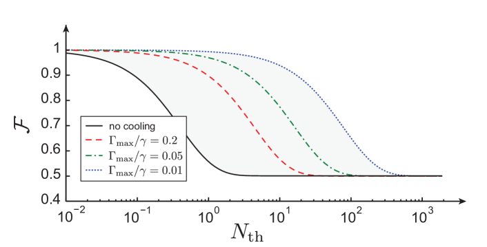
As a specific example, we consider a potential realization of phonon networks using the on-chip OM structures discussed in reference [25]. We assume local phonon modes of frequency GHz and a decay into the waveguide of MHz. For a quality factor the intrinsic decoherence rate is kHz. For these parameters we plot in figure 7 the fidelity for transferring the superposition state between two nodes of a phonon network as a function of and for different effective qubit decay rates . For the numerical simulations we have used the effective model with as obtained in equation (53) and with . The fidelity is defined as the overlap between the target state and the actual state after the transfer, i.e. . We see that compared to the case where no cooling is applied and the fidelity already drops significantly for , the presence of the OM noise filter can push this bound to much larger occupation numbers. In particular, in the example considered here, this means that instead of requiring temperatures of mK, the OM cooling scheme allows the implementation of high fidelity state transfer protocols at much more convenient liquid Helium temperatures K where . Note that for the assumed value of kHz, the total transfer time of s is compatible with decoherence times that are achievable with various different solid-state qubits. A few specific examples will be discussed below in section 6.
5 Phonon routers
In the previous sections we have studied the transfer of single excitations through a thermal phonon network assuming that two nodes are coupled in a unidirectional way. This situation is applicable only to specific setups, for example, when the two nodes are located at the two ends of a single waveguide. In general the emission of phonons into left and right propagating modes, reflection and interference effects, or imperfect routing of phonons through multi-port junctions in a 2D setting will limit the implementation of efficient state transfer protocols in larger networks. In optical networks, many of these problems can be overcome by using optical circulators and optical isolators for the directional routing of photons. In the context of OMS it has already been suggested to use the intrinsic non-linearity of OM interactions to induce non-reciprocal effects for light [35, 36]. In the following we describe a related scheme, which allows us to engineer coherent non-reciprocal effects for phonons, where the directionality is simply imposed by the phase difference between two optical driving fields.
5.1 A three-port phonon circulator
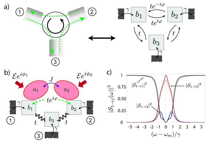
To illustrate the basic idea of a non-reciprocal phonon device let us consider the minimal setting of a three port circulator as shown in figure 8a. The localized phonon modes are mutually tunnel-coupled with a strength and coupled to phonon waveguides with a decay rate . The Hamiltonian is given by
| (54) |
assuming that the resonator frequencies are all equal. The crucial term in this setup is a complex tunneling amplitude between two of the resonators, which cannot be absorbed into local redefinitions of the . Therefore, this phase can be associated with an effective magnetic field for the phonon modes. Previously, such a setting has been described for superconducting microwave cavities, where the effective magnetic field can be engineered using superconducting qubits and external fluxes [44, 45]. Below we describe a non-magnetic approach to achieve this complex hopping amplitude in OMS.
Including the coupling to the waveguides and in a frame rotating with the resonator frequencies , the QLEs read
| (55) |
with the input-output relations . The above set of QLEs can be solved in Fourier space and the input-relation can be applied to obtain the full scattering matrix of this system. By choosing and , such that the decays into the waveguides are matched to the tunneling amplitudes, we find that for frequencies around ( in the rotating frame), the scattering matrix is given by
| (56) |
Up to factors , which can absorbed in the definitions of the operators, Eq. (56) describes a perfect circulator. For we obtain a similar result, but with the scattering direction reversed, i.e. , and . In figure 8c we plot the scattering probabilities , defined as , as a function of the frequency (relative to ) and for . We see the emergence of the ideal circulator relations close to resonance. We also find that these features are robust when we add an additional intrinsic loss rate .
5.2 Optomechanically engineered non-reciprocity for phonons
To implement a complex tunnel amplitude between two localized mechanical modes we propose a setup as shown in figure 8b. Here, the localized phonon mode is coupled to modes and mechanically with a (real) tunneling amplitude , while the tunneling between and is mediated by two driven optical cavities. The Hamiltonian for this system is
| (57) |
In the frame rotating with the frequency of an external driving field the Hamiltonian for the two coupled optical cavities is
| (58) |
where are the strengths and the phases of the optical driving fields. Finally,
| (59) |
describes the local OM interactions.
As discussed in section 3, in the limit of strong driving we can change to a displaced representation and linearize the OM coupling around the classical expectation values . In the present case the classical field amplitudes are given by
| (60) | |||||
| (61) |
where we have assumed that both cavities decay with the same rate rate and we have absorbed non-linear shifts of the detunings by a redefinition of . We write and obtain the linearized OM coupling
| (62) |
Note that for given , and the external control parameters and provide enough flexibility to independently adjust the phases and keep .
We focus on the specific case , and introduce symmetric and anti-symmetric optical modes with detunings . Further, we assume that , which allows us to make a rotating wave approximation with respect to . Then, after changing to a frame rotating with , the total Hamiltonian is given by
| (63) |
where . In a final step we assume and treat the OM coupling using second-order perturbation theory. Apart from small frequency shifts for the mechanical modes this results in an effective tunneling Hamiltonian
| (64) |
where and
| (65) |
Thus, by choosing the external control parameters such that and that matches the bare mechanical tunneling amplitude , the setup shown in figure 8b realizes a switchable three-port phonon circulator as discussed in the previous subsection. Note that the interaction with the optical modes also introduces an additional decay channel with rate , where . Compared to the noise filtering scheme described above, this requires slightly lower cavity decays satisfying .
As a specific example let us consider the phonon waveguide scenario discussed above with typical phonon frequencies GHz and a phonon-waveguide coupling of MHz. If we choose we obtain and the conditions can be achieved for MHz and GHz. For the same parameters a value of MHz is sufficient to suppress the optically induced decay rate below the value shown in figure 8c. This is only slightly below demonstrated values for in state of the art OM crystal cavities [22, 25].
6 Implementations
The fabrication and control of mechanical systems, resonator arrays and phonon waveguides as well as their coupling to other microscopic quantum systems (qubits) is currently a very active field of research. For many of these systems the general control techniques described in this work could provide the basis for phonon-based quantum communication applications or mechanical quantum interfaces in hybrid qubit setups. In the following we present a brief discussion of several potential candidate systems for implementing phonon networks.
6.1 Phonon channels
As described in section 2, a 1D phonon channel can be realized by fabricating a large array of coupled nanomechanical resonators with a bare frequency and nearest neighbor coupling . This scenario has been experimentally studied, for example in reference [37], where the resonators were charged up and coupled via electrostatic interactions. Alternatively, the resonators can also be coupled mechanically via bridges or the support [46]. Both approaches are suitable for realizing phonon channels with frequencies ranging from MHz to a few 100 MHz, where also very high Q-values around are nowadays routinely achieved. At mK this frequency range corresponds to a few tens to a few hundred thermal phonons, which can still be efficiently suppressed using the proposed OM noise filtering scheme.
A more practical and very versatile approach for implementing phonon waveguides based on phononic bandgap materials has recently attracted increasing attention [32, 33]. Here, a 2D structure with periodically varying mechanical properties is designed such that a complete band gap in the mechanical dispersion relation appears. Then, phonon wave guides can be realized by introducing line-defects in these structures, to which the phonons are confined as long as their frequency lies within the bandgap of the bulk phononic crystal. With this approach phonon waveguides with frequencies GHz can be realized, where even at K the thermal occupation of the waveguide is only a few tens of quanta. Further, as indicated in Figure 1b, such waveguides can be easily combined with localized phonon cavities and integrated OM devices [25].
6.2 Qubit-phonon interfaces
The implementation of phonon quantum networks also requires the realization of coherent and controllable interfaces between mechanics and stationary qubits. Here the ability of mechanical systems to respond to weak optical, electrical and magnetic forces enables the coupling of mechanical resonators to a large variety of spin or charge based qubits and a few prototype examples are outlined in the following.
6.2.1 Spin qubits.
Qubits encoded in localized spin degrees of freedom, for example in spins associated with Nitrogen vacancy (NV) impurities in diamond [47] or phosphor donors in silicon [48], can be coupled to mechanical motion using magnetized tips [13, 14, 49]. A strong magnetic field gradient from the tip induces a position dependent Zeeman shift of the spin resulting in an interaction of the form
| (66) |
Here GHz is the bare spin splitting and is the Zeeman shift per zero point motion , where and is the Bohr magneton. For nano-scale mechanical resonators with frequencies in the few MHz regime this coupling can be substantial and reach values kHz [50]. Base on this coupling the use of mechanical transducers to mediate spin-spin interactions in small resonator arrays has been proposed previously [23], and the present techniques can be used to extend these ideas to larger networks. To achieve an effective Jaynes-Cummings type interaction as given in Eq. (2), the spin is driven by a near resonant microwave field with frequency and Rabi frequency as described by the last term in Eq. (66). Then, by changing into a dressed spin basis and making a rotating wave approximation with respect to , the effective interaction is given by [43, 50]
| (67) |
where and . The qubit-resonator coupling can be controlled by adiabatically varying the effective detuning or the mixing angle .
Instead of using external magnetic field gradients, alternative schemes to strongly couple spins to mechanical motion have been recently suggested for carbon nanotubes [51, 52]. Here a single electron is localized on the nanotube and couples to its vibration via spin-orbit interactions. In this case even larger couplings MHz and larger mechanical frequencies MHz are achievable. Although a controlled fabrication and positioning of carbon nanotubes is still challenging, a phonon quantum bus could be realized by electrically coupling the nanotube to other mechanical resonators, which can be fabricated in a more controlled manner.
6.2.2 Superconducting qubits.
The coupling of nanomechanical systems to various types of superconducting qubits has been demonstrated in recent experiments [9, 12, 53]. While for superconducting qubits other ways for communication exist, for example via microwave transmission lines, the coupling to phononic channels could still be interesting for creating interfaces to other quantum systems, especially to optical qubits for long-distance quantum communication [24, 25]. Depending on the type of qubit (‘charge’, ‘phase’, ‘flux’, …) the qubit-resonator interaction can be due to electrostatic [17, 54], piezo-electric [9] or magnetic interactions [55, 56, 57], and can in all three cases be substantially larger than in the case of spin qubits. Since the bare transition frequency of superconducting qubits is typically in the GHz regime, a resonant coupling to mechanical systems in the MHz range can again be achieved as described above, namely by applying additional driving fields to compensate for the frequency mismatch [54, 58]. Alternatively, superconducting qubits could be coupled directly to high frequency mechanical modes as demonstrated in Ref. [9].
6.2.3 Quantum dots and defect centers.
The bending of a mechanical resonator locally deforms the lattice configuration of the host material and by that shifts the electronic states associated with artificial quantum dots or naturally occurring defect centers in solids. In the bulk this deformation potential interaction is usually responsible for line broadening of optical transitions and other decoherence effects, but in the case of confined modes it can also lead to a significant coherent coupling to single phonons. In Ref. [59] the coupling of a quantum dot to the fundamental bending mode of a doubly clamped beam has been considered, leading to a deformation potential coupling of the form
| (68) |
where denotes the electronically excited state, the beam length, its thickness and the zero point motion. The and are deformation potential constants for the ground and excited electronic states and for typical values eV and micron sized beams a coupling strength of MHz can be achieved. This is already comparable to the radiative lifetime of the electronically excited state, but can in principle be pushed to values GHz using much smaller, phononic Bragg-cavities as suggested in Ref. [60].
As a potential scenario where the deformation potential interactions could be used to implement a controllable qubit phonon interface, we consider an NV center embedded in a diamond nanoresonator. The electronic ground state of the NV defect is a spin triplet, where two states and can be used to encode quantum information. The qubit states in the electronic ground state, which are highly immune against external perturbations, can be coupled via an optical Raman process involving an electronically excited state, which, in contrast, is strongly coupled to phonons [61]. In D we adiabatically eliminate the dynamics of the excited state and derive an effective spin-phonon interaction of the form
| (69) |
Here the are Pauli operators for the qubit subspace and for optimized laser detunings is a tunable coupling where are the optical Rabi frequencies. Note that this coherent interaction is accompanied by dissipation at an average rate and the ratio is not affected by the off-resonant Raman coupling. This is in contrast to cavity QED where the optical field couples to the atomic coherence and not to the population of the excited state as described by .
7 Conclusions and outlook
In summary we have described the implementation of dissipative as well as coherent OM control elements for realizing quantum communication protocols in extended phononic networks. We have shown how OM continuous mode cooling schemes can be used to create a cold frequency window in the thermal noise spectrum of a phononic channel and we have analyzed the fidelity of quantum state transfer protocols under these conditions. Further, we have proposed the realization of non-reciprocal phononic elements, which rely on strong coherent OM interactions and where the directionality is simply controlled by the phase of an external laser field. Based on this principle, various switches and routers for propagating phonons can be constructed, which allow for the implementation of efficient quantum communication protocols also in larger phonon networks.
Both the OM noise filter as well as the phonon router can be realized with state-of-the-art mechanical systems. Combined with the ongoing developments in the control of qubit-resonator interactions, they could soon provide the elemental tools for implementing phononic quantum networks. As potential applications of such networks we envision the distribution of entanglement within a larger quantum computing architecture, where propagating phonons can replace or complement direct qubit shuttling techniques [62, 63]. Here the ability of mechanical systems to interact with various different types of qubits, makes phononic channels particularly suited for hybrid qubit settings. Beyond quantum communication applications, the OM control techniques described here may also be used to probe the propagation and scattering of single-phonon wave packets.
Acknowledgments
The authors would like to thank S. Bennett, F. Marquardt, O. Painter, A. Safavi-Naeini for stimulating discussions. This work was supported by the EU network AQUTE and the Austrian Science Fund (FWF) through SFB FOQUS and the START grant Y 591-N16. M.L. acknowledges support by NSF, CUA, DARPA and the Packard Foundation.
Appendix A Coupled resonator arrays
In this appendix we derive the effective propagation equations and input-output relations for phononic quantum channels consisting of a large array of coupled mechanical resonators. Assuming a homogenous system the resonator array is described by the Hamiltonian
| (70) |
and the equations of motion for the position operators are given by
| (71) |
where is the nearest neighbor phonon-phonon coupling strength. For a large array we can assume periodic boundary conditions and write
| (72) |
where are bosonic operators for the plane wave modes labeled by and normalized to . The eigenfrequencies are given by
| (73) |
We are interested in the regime where the total length as well as the other relevant scales of the network are large compared to the spacing between the individual resonators. We introduce a continuous field
| (74) |
such that . The quasi-momentum is restricted to the first Brillouin zone and .
To proceed we now consider the tight binding limit , where and the phonon modes form a band of width around a large center frequency . Further, for frequencies around the dispersion relation is approximately linear and can be written as
| (75) |
where is the sound velocity and a frequency offset. Therefore, as long as we are interested in the dynamics of phonon modes away from the band edges we can set and approximate the displacement field by
| (76) |
Here and the field is normalized to
| (77) |
where and . The field operators can be decomposed into a right- and a left-moving component , as defined in equations (4) and (5).
The coupling of the localized phonon modes to the phonon channel can be written as
| (78) |
where is non-zero only for site , which are next to a local mode (we can assume side-coupled resonators, such there is only one neighbor). We define where the zero point motion of the local mode. Then, under the assumption that , we can make a RWA and obtain the coupling given in equation (6) with a resonator decay rate given by .
A.1 Propagation losses
To model propagation losses in the phonon waveguide we add an intrinsic loss channel with rate for each of the waveguide modes. Making the RWA right from the beginning, the dynamics of the whole resonator array is modeled by the coupled QLEs,
| (79) |
where is the bosonic operator for the mechanical resonator at site and the are uncorrelated thermal noise operators . In the corresponding momentum representation and , the coupling is diagonal
| (80) |
where as above . From this equation we obtain the propagation equation for the right moving field ,
| (81) |
Here the thermal noise field is defined as
| (82) |
such that it is normalized .
Appendix B Optomechanical cooling
After linearizing the OM coupling the QLEs (13) and (14) can be written as
| (83) |
where we have grouped operators as , and . The matrix is given by
| (84) |
We define the Fourier-transformed operators as , and obtain
| (85) |
where we set and now , etc. The non-vanishing correlations of the noise operators are , and , within the relevant frequency range. Then, the stationary fluctuation spectrum of the mechanical mode is given by
| (86) |
Under the weak coupling and sideband resolved condition this expression simplifies to the result given in equation (17).
In section 3.3 we are interested in spectrum of the scattered field in the case where the OMS is in addition coupled to the phonon waveguide with rate . We define and the intrinsic noise as above, but we set . The input-output relations can then be written as where is a diagonal matrix. Then, together with equation (85) we obtain
| (87) |
where and and in the definition of we replaced . The filtered noise spectrum of the out-field is given by
| (88) |
where in equation (28) the approximation has been made.
B.1 Multi-mode cooling
We can use the same approach to solve for the stationary state of the multimode system described in section 3.2. In the following we assume for simplicity the validity of the RWA, such that the QLEs for the equations for the annihilation operators form a closed set
| (89) |
where now and and the matrix can be derived from equations (19)-(22). Following the same steps as above we obtain
| (90) |
which we have used to evaluate the multi-mode cooling results presented in figure 4c.
Appendix C Cascaded master equation
To simulate the state transfer between two nodes in the presence of incident noise and OM cooling, we map the qubit QLEs (38) and (39) with time dependent decay rates and onto an equivalent cascaded master equation [38], which we can then integrate numerically. Since we cannot treat the filtered input noise directly using a master equation we consider a unidirectional network where the OM cooled phonon cavity is included as a first system. The OM cooling is modeled by an additional decay channel for the phonon cavity at a rate , which is matched to the decay rate of the phonon cavity into the waveguide. The cascaded master equation, which describes this system is given by
| (91) |
where . By identifying , and the collective operator and . is the thermal occupation number of the incident white noise.
Appendix D NV-phonon coupling
In this appendix we show how for an NV center in diamond the deformation potential coupling can be used to realize the effective spin-phonon interaction (69). The NV center has triplet ground state and we assume that the qubit is encoded in the states and . The qubit states are coupled by external laser fields to an electronically excited state , which is coupled to the deformation of the local lattice structure induced by the vibration of the beam. In the frame rotating with the laser frequencies the Hamiltonian is given by
| (92) |
where the are tunable Rabi frequencies and we have chosen the zero of energy to coincide with the excited state level such that and are detunings of the drive lasers from the to and to transitions, respectively. The interaction term can be eliminated by a polaron transformation
| (93) |
which transforms the Hamiltonian into
| (94) |
and is still exact. Since the ratio , we can expand to first order in and obtain .
Our goal is to induce a coherent Raman transition from state to state while simultaneously absorbing a phonon from the nanomechanical oscillator. To make this process resonant we set and , where is the overall detuning. We change into an interaction picture with respect to and write the total state as . The equations of motion are then given by
| (95) | |||||
| (96) |
where we have added an imaginary part to model the radiative decay of the exited state with rate 222For simplicity we here omit the associated recycling terms, which can be included, for example, using a stochastic wavefunction formalism [38].. Assuming that , we can approximately integrate the equation of motion for ,
| (97) |
and insert this result back into the equations of motion for . By keeping only non-rotating terms, we obtain for the subspace,
| (98) |
and a similar result for the evolution of . In the limit and using the definition , we can identify an effective spin-phonon coupling and effective decay rates for each spin level,
| (99) |
The ratio between the coherent coupling and the mean decay rate is optimized for where .
Here we have assumed that the NV center is coupled to a single vibrational mode. In general, nanostructured resonators will support multiple mechanical modes so that the phononic part in the Hamiltonian (92) generalizes to . However, since the higher-frequency modes of nanostructured resonators are separated from the fundamental mode by GHz, the other modes are highly off-resonant and their contributions to the resulting spin-phonon coupling are negligibly small. See reference [59] for a similar discussion.
References
References
- [1] C Höhberger Metzger and K Karrai. Cavity cooling of a microlever. Nature, 432:1002–5, 2004.
- [2] S Gigan, H R Böhm, M Paternostro, F Blaser, G Langer, J B Hertzberg, K C Schwab, D Bäuerle, M Aspelmeyer, and A Zeilinger. Self-cooling of a micromirror by radiation pressure. Nature, 444:67–70, 2006.
- [3] O Arcizet, P-F Cohadon, T Briant, M Pinard, and A Heidmann. Radiation-pressure cooling and optomechanical instability of a micromirror. Nature, 444:71–74, 2006.
- [4] D Kleckner and D Bouwmeester. Sub-kelvin optical cooling of a micromechanical resonator. Nature, 444:75–8, 2006.
- [5] T Corbitt, C Wipf, T Bodiya, D Ottaway, D Sigg, N Smith, S Whitcomb, and N Mavalvala. Optical dilution and feedback cooling of a gram-scale oscillator to 6.9 mK. Phys. Rev. Lett., 99:160801, 2007.
- [6] J D Thompson, B M Zwickl, A M Jayich, F Marquardt, S M Girvin, and J G E Harris. Strong dispersive coupling of a high-finesse cavity to a micromechanical membrane. Nature, 452:72–5, 2008.
- [7] A Schliesser, R Rivière, G Anetsberger, O Arcizet, and T J Kippenberg. Resolved-sideband cooling of a micromechanical oscillator. Nat Phys, 4:415–9, 2008.
- [8] D J Wilson, C A Regal, S B Papp, and H J Kimble. Cavity optomechanics with stoichiometric SiN films. Phys. Rev. Lett., 103:207204, 2009.
- [9] A D O’Connell, M Hofheinz, M Ansmann, R C Bialczak, M Lenander, E Lucero, M Neeley, D Sank, H Wang, M Weides, J Wenner, J M Martinis, and A N Cleland. Quantum ground state and single-phonon control of a mechanical resonator. Nature, 464:697–703, 2010.
- [10] J D Teufel, T Donner, D Li, J W Harlow, M S Allman, K Cicak, A J Sirois, J D Whittaker, K W Lehnert, and R W Simmonds. Sideband cooling of micromechanical motion to the quantum ground state. Nature, 475:359–63, 2011.
- [11] J Chan, T P Mayer Alegre, A H Safavi-Naeini, J T Hill, A Krause, S Gröblacher, M Aspelmeyer, and O Painter. Laser cooling of a nanomechanical oscillator into its quantum ground state. Nature, 478:89–92, 2011.
- [12] M D LaHaye, J Suh, P M Echternach, K C Schwab, and M L Roukes. Nanomechanical measurements of a superconducting qubit. Nature, 459:960–4, 2009.
- [13] O Arcizet, V Jacques, A Siria, P Poncharal, P Vincent, and S Seidelin. A single nitrogen-vacancy defect coupled to a nanomechanical oscillator. Nat Phys, 7:879–83, 2011.
- [14] S Kolkowitz, A C Bleszynski Jayich, Q Unterreithmeier, S D Bennett, P Rabl, J G E Harris, and M D Lukin. Coherent sensing of a mechanical resonator with a single-spin qubit. Science, 355:1603–6, 2012.
- [15] V Fiore, Y Yang, M C Kuzyk, R Barbour, L Tian, and H Wang. Storing optical information as a mechanical excitation in a silica optomechanical resonator. Phys. Rev. Lett., 107:133601, 2011.
- [16] E Verhagen, S Deléglise, S Weis, A Schliesser, and T J Kippenberg. Quantum-coherent coupling of a mechanical oscillator to an optical cavity mode. Nature, 482:63–7, 2012.
- [17] A D Armour, M P Blencowe, and K C Schwab. Entanglement and decoherence of a micromechanical resonator via coupling to a cooper-pair box. Phys. Rev. Lett., 88:148301, 2002.
- [18] W Marshall, C Simon, R Penrose, and D Bouwmeester. Towards quantum superpositions of a mirror. Phys. Rev. Lett., 91:130401, 2003.
- [19] O Romero-Isart, A C Pflanzer, F Blaser, R Kaltenbaek, N Kiesel, M Aspelmeyer, and J I Cirac. Large quantum superpositions and interference of massive nanometer-sized objects. Phys. Rev. Lett., 107:020405, 2011.
- [20] I Pikovski, M R Vanner, M Aspelmeyer, M S Kim, and C Brukner. Probing planck-scale physics with quantum optics. Nat Phys, 8:393-7, 2012.
- [21] S Weis, R Rivière, S Deléglise, E Gavartin, O Arcizet, A Schliesser, and T J Kippenberg. Optomechanically induced transparency. Science, 330:1520–3, 2010.
- [22] A H Safavi-Naeini, T P Mayer Alegre, J Chan, M Eichenfield, M Winger, Q Lin, J T Hill, D E Chang, and O Painter. Electromagnetically induced transparency and slow light with optomechanics. Nature, 472:69–73, 2011.
- [23] P Rabl, S J Kolkowitz, F H L Koppens, J G E Harris, P Zoller, and M D Lukin. A quantum spin transducer based on nanoelectromechanical resonator arrays. Nat Phys, 6:602–8, 2010.
- [24] K Stannigel, P Rabl, A S Sørensen, P Zoller, and M D Lukin. Optomechanical transducers for long-distance quantum communication. Phys. Rev. Lett., 105:220501, 2010.
- [25] A H Safavi-Naeini and O Painter. Proposal for an optomechanical traveling wave phonon–photon translator. New Journal of Physics, 13:013017, 2011.
- [26] J I Cirac and P Zoller. Quantum computations with cold trapped ions. Phys. Rev. Lett., 74:4091–4, 1995.
- [27] J Eisert, M B Plenio, S Bose, and J Hartley. Towards quantum entanglement in nanoelectromechanical devices. Phys. Rev. Lett., 93:190402, 2004.
- [28] M Schmidt, M Ludwig, and F Marquardt. Optomechanical circuits for nanomechanical continuous variable quantum state processing. arXiv:1202.3659, 2012.
- [29] J I Cirac, P Zoller, H J Kimble, and H Mabuchi. Quantum state transfer and entanglement distribution among distant nodes in a quantum network. Phys. Rev. Lett., 78:3221–4, 1997.
- [30] H J Kimble. The quantum internet. Nature, 453:1023–30, 2008.
- [31] S Ritter, C Nolleke, C Hahn, A Reiserer, A Neuzner, M Uphoff, M Mucke, E Figueroa, J Bochmann, and G Rempe. An elementary quantum network of single atoms in optical cavities. Nature, 484:195–200, 2012.
- [32] R H Olsson III and I El-Kady. Microfabricated phononic crystal devices and applications. Measurement Science and Technology, 20:012002, 2009.
- [33] A H Safavi-Naeini and O Painter. Design of optomechanical cavities and waveguides on a simultaneous bandgap phononic-photonic crystal slab. Opt. Express, 18:14926–43, 2010.
- [34] B Lüthi. Physical acoustics in the solid state. Springer series in solid state sciences. Springer, Berlin, 2005.
- [35] S Manipatruni, J T Robinson, and M Lipson. Optical nonreciprocity in optomechanical structures. Phys. Rev. Lett., 102:213903, 2009.
- [36] M Hafezi and P Rabl. Optomechanically induced non-reciprocity in microring resonators. Opt. Express, 20:7672–84, 2012.
- [37] E Buks and M L Roukes. Electrically tunable collective response in a coupled micromechanical array. Microelectromechanical Systems, Journal of, 11:802–7, 2002.
- [38] C W Gardiner and P Zoller. Quantum Noise. Springer, Berlin, 2004.
- [39] F Marquardt, J P Chen, A A Clerk, and S M Girvin. Quantum theory of cavity-assisted sideband cooling of mechanical motion. Phys. Rev. Lett., 99:093902, 2007.
- [40] I Wilson-Rae, N Nooshi, W Zwerger, and T J Kippenberg. Theory of ground state cooling of a mechanical oscillator using dynamical backaction. Phys. Rev. Lett., 99:093901, 2007.
- [41] C K Law. Interaction between a moving mirror and radiation pressure: A hamiltonian formulation. Phys. Rev. A, 51:2537–2541, 1995.
- [42] T J Kippenberg and K J Vahala. Cavity opto-mechanics. Opt. Express, 15(25):17172–17205, 2007.
- [43] K Stannigel, P Rabl, A S Sørensen, M D Lukin, and P Zoller. Optomechanical transducers for quantum-information processing. Phys. Rev. A, 84:042341, 2011.
- [44] J Koch, A A Houck, K Le Hur, and S M Girvin. Time-reversal-symmetry breaking in circuit-qed-based photon lattices. Phys. Rev. A, 82:043811, 2010.
- [45] A Nunnenkamp, J Koch, and S M Girvin. Synthetic gauge fields and homodyne transmission in jaynes–cummings lattices. New Journal of Physics, 13:095008, 2011.
- [46] R B Karabalin, M C Cross, and M L Roukes. Nonlinear dynamics and chaos in two coupled nanomechanical resonators. Phys. Rev. B, 79:165309, 2009.
- [47] F Jelezko and J Wrachtrup. Single defect centres in diamond: A review. Physica Status Solidi A, 203:3207, 2006.
- [48] A M Tyryshkin, S Tojo, J J L Morton, H Riemann, N V Abrosimov, P Becker, H-J Pohl, T Schenkel, M L W Thewalt, K M Itoh, and S A Lyon. Electron spin coherence exceeding seconds in high-purity silicon. Nat Mater, 11:143, 2012.
- [49] H J Mamin, M Poggio, C L Degen, and D Rugar. Nuclear magnetic resonance imaging with 90-nm resolution. Nat. Nanotechnol., 2:301–6, 2007.
- [50] P Rabl, P Cappellaro, M V Gurudev Dutt, L Jiang, J R Maze, and M D Lukin. Strong magnetic coupling between an electronic spin qubit and a mechanical resonator. Phys. Rev. B, 79:041302, 2009.
- [51] A Palyi, P R Struck, M Rudner, K Flensberg, and G Burkard. Spin-orbit induced strong coupling of a single spin to a nanomechanical resonator. Phys. Rev. Lett., 108:206811, 2012.
- [52] C Ohm, C Stampfer, J Splettstoesser, and M R Wegewijs. Readout of carbon nanotube vibrations based on spin-phonon coupling. Appl. Phys. Lett., 100:143103, 2012.
- [53] S Etaki, M Poot, I Mahboob, K Onomitsu, H Yamaguchi, and H S J van der Zant. Motion detection of a micromechanical resonator embedded in a d.c. squid. Nature Physics, 4:785, 2008.
- [54] I Martin, A Shnirman, L Tian, and P Zoller. Ground-state cooling of mechanical resonators. Phys. Rev. B, 69:125339, 2004.
- [55] X Zhou and A Mizel. Nonlinear coupling of nano mechanical resonators to josephson quantum circuits. Phys. Rev. Lett., 97:267201, 2006.
- [56] F Xue, Y D Wang, C P Sun, H Okamoto, H Yamaguchi, and K Semba. Controllable coupling between flux qubit and nanomechanical resonator by magnetic field. New Journal of Physics, 9:35, 2007.
- [57] K Jaehne, K Hammerer, and M Wallquist. Ground-state cooling of a nanomechanical resonator via a cooper-pair box qubit. New Journal of Physics, 10:095019, 2008.
- [58] P Rabl, A Shnirman, and P Zoller. Generation of squeezed states of nanomechanical resonators by reservoir engineering. Phys. Rev. B, 70:205304, 2004.
- [59] I Wilson-Rae, P Zoller, and A Imamoḡlu. Laser cooling of a nanomechanical resonator mode to its quantum ground state. Phys. Rev. Lett., 92:075507, 2004.
- [60] Ö O Soykal, R Ruskov, and C Tahan. Sound-based analogue of cavity quantum electrodynamics in silicon. Phys. Rev. Lett., 107:235502, 2011.
- [61] J R Maze, A Gali, E Togan, Y Chu, A Trifonov, E Kaxiras, and M D Lukin. Properties of nitrogen-vacancy centers in diamond: the group theoretic approach. New Journal of Physics, 13:025025, 2011.
- [62] D Kielpinski, C Monroe, and D J Wineland. Architecture for a large-scale ion-trap quantum computer. Nature, 417:709, 2002.
- [63] J M Taylor, H A Engel, W Dur, A Yacoby, C M Marcus, P Zoller, and M D Lukin. Fault-tolerant architecture for quantum computation using electrically controlled semiconductor spins. Nature Physics, 1:177, 2005.