A Test for Radial Mixing Using Local Star Samples

Abstract

We use samples of local main-sequence stars to show that the radial gradient of [Fe/H] in the thin disk of the Milky Way decreases with mean effective stellar temperature. Many of these stars are visiting the solar neighborhood from the inner and outer Galaxy. We use the angular momentum of each star about the Galactic center to determine the guiding center radius and to eliminate the effects of epicyclic motion, which would otherwise blur the estimated gradients. We interpret the effective temperature as a proxy for mean age, and conclude that the decreasing gradient is consistent with the predictions of radial mixing due to transient spiral patterns. We find some evidence that the trend of decreasing gradient with increasing mean age breaks to a constant gradient for samples of stars whose main-sequence life-times exceed the likely age of the thin disk.

1 Introduction

A radial abundance gradient in the Milky Way disk today is well-established from analyses of the interstellar medium (Shaver et al., 1983; Balser et al., 2011). Metal abundances are believed to increase over time and most chemical evolution models (e.g., Boissier & Prantzos, 1999; Hou et al., 2000; Chiappini et al., 2001; Naab & Ostriker, 2006; Fu et al., 2009) predict that a radial abundance gradient is created early and may even have been steeper in the past. This picture is consistent with “inside-out” disk formation, in which the stellar population at increasing radii is younger and more metal poor (e.g. de Jong, 1999; Muñoz-Mateos et al., 2007).

The chemical composition of a star is that of the cloud of gas from which it formed. Abundance gradients are therefore also observed in the disk of the Milky Way in stars (Nordström et al., 2004; Haywood, 2008; Luck et al., 2011; Schlesinger et al., 2011), in planetary nebulae (Maciel et al., 2007; Stanghellini & Haywood, 2010), and in open star clusters (Friel et al., 2002; Chen et al., 2003). While all agree that abundances in the thin disk decrease outwards, the precise slope differs from sample to sample and element measured.

The orbits of disk stars generally become more eccentric over time (Wielen, 1977; Holmberg et al., 2009; Aumer & Binney, 2009), which “blurs” measurements of the metallicity gradient when the instantaneous radii of older stars are used. Eccentric motion of any amplitude, projected to the mid-plane of an axisymmetric potential, can be described as a retrograde epicycle about a guiding center that orbits at a constant angular rate (Binney & Tremaine, 2008). The guiding center, or home, radius of a disk star is directly related to the $z$-component of the angular momentum, $L_{z}$, about the Galactic center and, since angular momentum is conserved, can be determined from any point around the epicycle. Thus measurement of the angular momenta of stars allows us to eliminate the blurring effects of epicyclic motions and simplifies the interpretation of metallicity gradients. Nordström et al. (2004) used the mean Galacto-centric radius for the same reason, which requires integrating the orbit in some adopted potential – angular momentum is more direct.

In the absence of radial mixing, chemical evolution models in which the metallicity of the ISM increases at each radius over time would predict a tight correlation between the metallicity and age for stars of a given home radius. This prediction is not supported by the data, and the metallicity distribution of all but the youngest stars shows a broad distribution (Edvardsson et al., 1993; Nordström et al., 2004), which persists even after correcting for epicyclic blurring (Haywood, 2008).

Sellwood & Binney (2002) argued that stars in a disk galaxy are shuffled in radius over time by the effects of transient spiral arms. They showed that a star near the corotation resonance of a spiral could gain or lose enough angular momentum for its home radius to change by up to 2 kpc, leaving the star at its new mean galacto-centric distance with no increase in its epicyclic amplitude. The resulting radial mixing is described as “churning” and their result has been confirmed and extended (Ros̆kar et al., 2008a, b; Loebman et al., 2011; Minchev et al., 2011; Bird et al., 2012; Solway et al., 2012). The broad spread of metallicities among stars having common ages and home radii today is then naturally explained as reflecting the past gradient of metallicity of the ISM at their various birth radii. Schönrich & Binney (2009) provide a model for chemical evolution of the Milky Way that was the first to include radial mixing. Loebman et al. (2011) find good agreement between the predictions of their simulations, that manifest substantial radial mixing, with the metallicity distribution of stars from the SDSS (Ivezić et al., 2008); Lee et al. (2011) find other evidence supporting radial migration.

An additional consequence of radial mixing, or churning, is that the radial metallicity gradient of a generation of stars is gradually flattened over time. Nordström et al. (2004) and Haywood (2008), from local stars suggest that the gradient may become shallower with increasing age. Casagrande et al. (2011) report little evolution of the radial metallicity gradient over the past $\sim 5~{}$Gyr, using infrared magnitudes and improved models to revise the age estimates for the stars in the Nordström et al. (2004) sample. Estimating the age of an individual star (see Soderblom, 2010, for a recent review) is a delicate art and the results even for well-observed main-sequence stars can be contentious (e.g. Reid et al., 2007; Holmberg et al., 2007). Furthermore, the evidence from star clusters (Friel et al., 2002; Chen et al., 2003) suggests that the radial metallicity gradient may steepen with age, in line with inside-out models of galaxy formation. Maciel et al. (2007), from a study of planetary nebulae abundance data, also find evidence for a steeper gradient among their older objects, although Stanghellini & Haywood (2010) reach the opposite conclusion that older PNe show a shallower gradient. We comment on these apparently conflicting results in §4.2.

Here we study the age-dependence of the metallicity gradient using a sample of stars in the solar neighborhood. Instead of estimating ages of individual stars, we adopt the effective temperature of a collection of main sequence stars as a proxy for their mean age, in the same manner that Aumer & Binney (2009) used color. Since the main-sequence lifetime of a star is shorter for hotter stars, the mean ages of main sequence disk stars grouped by effective temperature must be lower for the hotter groups. (Of course, this argument requires the reasonable assumptions that stars have been forming with an approximately constant IMF and at a roughly uniform rate over the lifetime of the Milky Way disk.) The trend of increasing mean age with decreasing temperature must change to a constant at the point at which the main-sequence lifetimes of stars exceed the age of the disk. Note that the main-sequence turn-off for stars of age 10 Gyr occurs for $5\,500\lesssim T_{\rm eff}\lesssim 6\,000\;$K over the range $0.4\gtrsim\;$[Fe/H]$\;\gtrsim-0.5$ (Demarque et al., 2004).

As explained above, we eliminate epicyclic blurring by estimating the specific angular momentum of each star, which requires knowledge of its full 6D phase space coordinates: i.e. distance and proper motion, as well as radial velocity and sky position. A radial velocity can be measured spectroscopically at any distance, but a reliable distance can be obtained only for nearby stars. Furthermore, distance uncertainties factor into velocity components in the sky plane adding to the desirability of restricting attention to stars close to the Sun. Also, by focusing on nearby stars, any variations in $L_{z}$ across our sampling volume due to possible departures from axisymmetry in the Galactic potential will be negligible.

A benefit of stellar epicycle excursions is that they bring stars to the solar neighborhood. Thus a sample of very local stars will span a significant range of specific angular momenta and, therefore, home radii.

In this paper, we assemble a sample of local, main-sequence stars having estimated effective temperatures, metallicities and full space motions. We draw these stars from three sources as described in the next section.

2 Star samples

2.1 Geneva-Copenhagen sample

The Geneva-Copenhagen survey of nearby stars (Nordström et al., 2004) used Hipparcos positions and proper motions, supplemented by spectroscopic observations, to construct a homogeneous sample of nearby mostly F and G dwarf stars. We employ their updated catalog (Holmberg et al., 2009) that uses their revised temperature calibration and the improved astrometry from the reanalysis of Hipparcos data by van Leeuwen (2007). This monumental effort has resulted in a large sample of stars in the solar neighborhood with distances and full space motions. Holmberg et al. (2009) do not supply individual uncertainties for each velocity, but assert that they are believed accurate to 1.5 km s^-1, with the greatest contribution coming from distance uncertainties.

The machine readable table of $16\,682$ stars made available by Holmberg et al. (2009) includes sky positions, distances, and the $(U,V,W)$ components of the star’s motion relative to the Sun in Galactic coordinates. We discard those having no distance, no $(U,V,W)$ velocities, or no estimate of $T_{\rm eff}$. We do not use the disputed age estimates (e.g. Reid et al., 2007; Holmberg et al., 2007) in the present paper. We correct for Solar motion relative to the local standard of rest (LSR) by adding $(U,V,W)_{\odot}=(11.10,12.24,7.25)\;$km s^-1 (Schönrich et al., 2010) to the tabulated velocities.

Nordström et al. (2004) note that they obtained [Fe/H]$\;\gtrsim 0.4$ for a small number of stars, though none is within 40 pc of the Sun. Furthermore, these high values are found only for stars with $T_{\rm eff}$$\;\gtrsim 6200\;$K. They argue that the coincidence of high $T_{\rm eff}$ and [Fe/H], together with other information, suggests that the extinction to these stars has been overestimated. We therefore discard a further 29 stars having [Fe/H]$\;>0.4$.

In order to select nearby disk stars, we further restrict the sample to stars whose best estimate of the distance is within $500\;$pc, $|U|,\;|V|<80\;$km s^-1, and retain only those having an energy of vertical motion about the Galactic mid-plane, $E_{z}=0.5(z^{2}\nu^{2}+W^{2})<392\;$(km s${}^{-1})^{2}$, with the vertical frequency $\nu=0.07\;$km s^-1 pc^-1 (Binney & Tremaine, 2008), giving them a maximum vertical excursion of $\pm 400\;$pc. Thus we select only stars that have a high probability of being thin disk stars, in the same spirit as Bensby et al. (2003), but not in exactly the same manner (see §4 for further discussion of selection effects). Our final sample contains $11\,877$ stars that we use in this analysis.

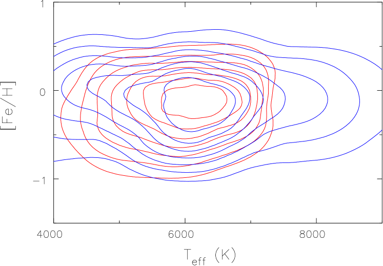
Figure 1: The densities of stars in the space of $T_{\rm eff}$ and [Fe/H] in our selected GCS (red) and RAVE (blue) subsamples.

The median distance of the selected stars is 75 pc and the sample within 40 pc of the Sun is believed to be near complete. We adopt $R_{0}=8\;$kpc, the circular speed of the LSR to be $V_{0}=220\;$km s^-1, and compute the Galacto-centric angular momentum, $L_{z}$, using the in-plane distance of the star from the Sun and the peculiar velocities $(U,V)$ corrected for the Sun’s motion.

The red contours in Fig. 1 show the distribution of the selected GCS stars in the space of $T_{\rm eff}$ and [Fe/H]. The range of $T_{\rm eff}$ indicates that the sample extends outside the spectral types F and G, reflecting the selection criteria described by Nordström et al. (2004). These authors estimate uncertainties of $\lesssim 0.1$ in [Fe/H] and 94 K in $T_{\rm eff}$.

Casagrande et al. (2011) present a recalibration of $T_{\rm eff}$ and [Fe/H] for the GCS stars that folds in the infrared flux from a star. They obtain slightly higher values for $T_{\rm eff}$ and [Fe/H] than those derived by Holmberg et al. (2009) and they too attempt to assign ages for the individual stars. The additional information used by Casagrande et al. (2011) should lead to improved values for the derived quantities, but they claim reliable results for fewer than half the GCS stars (their irfm sample) and for none of the cooler stars. We therefore continue to use the calibration for the whole GCS sample by Holmberg et al. (2009).

2.2 RAVE sample

The RAVE survey (Steinmetz et al., 2006) plans to measure the heliocentric radial velocities and stellar parameters for about a million stars in the southern sky having apparent magnitudes in the range $9<m_{I}<12$; the first $77\,461$ are available in the third data release (Siebert et al., 2011). The typical uncertainty in the radial velocity is $<2\;$km s^-1, but the distance to most stars has to be judged photometrically and most proper motions are from ground-based data. Thus three of the phase space coordinates for each star are of much lower quality than are those in the GCS, although this weakness will be compensated by a much larger sample size when the survey is complete.

We have downloaded the on-line table of the third data release from the RAVE website and selected a subset of stars for analysis. We estimate distances to these stars by fitting to the Yonsei-Yale isochrones (Demarque et al., 2004) using a method related to that described by Breddels et al. (2010, see also Burnett et al. 2011 for an alternative method). We adopt many of their selection criteria: we require the spectral signal-to-noise parameter S2N$\;>20$ with a blank spectral warning flag field; the parameters [M/H], log($g$), and $T_{\rm eff}$ to be determined; and the stars to have J and K_s magnitudes from 2MASS with no warning flags about the identification of the star or the 2MASS photometry. Unlike those authors, however, we have kept stars with $b<25\arcdeg$ on the grounds that extinction for the nearby stars that interest us will not be large enough in the near IR to severely bias our distance estimates. As we are here interested only in nearby main-sequence stars that are members of the disk population, we also make preliminary cuts to eliminate stars with log$(g)<4$, $T_{\rm eff}>10^{4}\;$K, and with $|v_{r}|>120\;$km s^-1. We have treated the tabulated [M/H] as equivalent to [Fe/H] since the corrections (Zwitter et al., 2008) are generally within the uncertainties. We also show in §2.3 that the [M/H] values for RAVE stars agree with the [Fe/H] values for the stars in common with the GCS.

We estimate the absolute J magnitude of each selected star by matching the estimated [Fe/H], log($g$), $T_{\rm eff}$, and J-K_s color to values in the isochrone tables for stars of all ages and all values of [$\alpha$/Fe], rejecting a few more stars for which the best match $\chi^{2}>6$. We consider the closest match in the tables to the given input parameters to yield the best estimate of the absolute magnitude from which we estimate a photometric distance using the apparent J-band magnitude. We save the values of [Fe/H], log($g$), $T_{\rm eff}$, and J-K_s color of the closest matching model star in the isochrone table; Monte-Carlo variation of the stellar parameters about this saved set of values suggests that distances have a fractional precision of 30% – 50%, with some larger uncertainties.

We use the proper motions in equatorial coordinates tabulated in RAVE, mostly from Tycho-2 (Høg et al., 2000), which we then combine with the radial velocity and position to determine the heliocentric velocity in Galactic components $(U,V,W)$ (Johnson & Soderblom, 1987; Piatek et al., 2002). We estimate uncertainties in these velocities from 500 Monte Carlo re-selections of all the stellar parameters that affect the distance estimate, adopting $\sigma({\rm J})=0.03\;$mag, $\sigma({\rm J-K}_{s})=0.042\;$mag, $\sigma(T_{\rm eff})=300\;$K, $\sigma(\log\,g)=0.3\;$dex, and $\sigma([{\rm Fe/H}])=0.25\;$dex (Breddels et al., 2010), as well as the tabulated radial velocity and proper motion uncertainties.

We exclude stars more distant than 500 pc, correct the space velocities for solar motion and apply the same restrictions as for the GCS sample to select only those with a high probability of being thin disk stars.

Figure 2: Histograms of distances and $L_{z}$ uncertainties for the selected sample of 9803 RAVE stars.

Fig. 2 shows histograms of distances and of uncertainties in $L_{z}$ for the $9,803$ remaining stars. The median distance is 220 pc from the Sun and uncertainties in $L_{z}$ are generally smaller than 5%.

The blue contours in Fig. 1 show the distribution of selected RAVE stars. The distribution in [Fe/H] values is slightly broader than for the GCS stars, reflecting in part at least the lower precision of the spectra. However, the rms scatter in [Fe/H] appears to be $\sim 0.2$, suggesting the uncertainty of 0.25 estimated by Siebert et al. (2011) is somewhat pessimistic for this sub-sample of main-sequence stars. These authors also suggest uncertainties of 300 K in their estimates of $T_{\rm eff}$, and the broader range of $T_{\rm eff}$ than in the GCS sample is therefore real.

2.3 Stars in common

The overlap between the GCS and RAVE samples of stars is quite small but, of those we have selected, precisely 100 stars are positionally coincident. This small degree of overlap allows us to compare the spectral parameters, $T_{\rm eff}$, [Fe/H], and radial velocity ($v_{r}$), derived separately by the two teams from their independent spectra.

We find that differences in the estimated $v_{r}$ for the same stars average just $0.32\;$km s^-1 higher in RAVE than in GCS, with an rms scatter about this mean of only $2.3\;$km s^-1. Similarly, differences in $T_{\rm eff}$ have a mean of 203 K, again higher in RAVE than in GCS, with an rms scatter about the mean of 202 K. Finally, the mean difference in [Fe/H] is 0.057, lower in RAVE than in GCS, with an rms scatter of 0.18. We have looked in vain for systematic variations of these differences, which appear to be consistent with random scatter.

Thus all three spectral parameters agree between the independent measures to an accuracy that is significantly better than expected from the quoted uncertainties, indicating that both teams have been very careful with their calibrations and conservative with their uncertainty estimates.

Figure 3: Histograms of distances and $L_{z}$ uncertainties for the selected sample of $11\,022$ M-dwarf stars.

2.4 M-dwarf sample

The SDSS (York et al., 2000) and Segue2 (Yanny et al., 2009) surveys are complete, but sample fainter stars than RAVE (the magnitude range for Segue2 was $14.0<g<20.3$) that are therefore generally more distant. Since the Sloan spectral parameters pipeline (Lee et al., 2008) does not attempt to fit stars with $T_{\rm eff}\lesssim 4500\;$K, almost all main sequence stars with estimated parameters in SDSS DR8 are more distant than 500 pc.

Fortunately, West et al. (2011) provided a catalog of 70 841 M-dwarfs from SDSS DR7. Their table provides a photometric estimate of the distance to each star, as well as a spectroscopic radial velocity, and proper motion from USNO-B/SDSS catalog (Munn et al., 2004, 2008). They suggest that distance uncertainties are typically about 20% and uncertainties in radial velocity are 7-10 km s^-1. None of these stars are in RAVE (because they are in different parts of the sky) and all are much cooler than the GCS stars.

As West et al. (2011) recommend, we selected stars with the “goodPM” and “goodPhot” flags set to ‘true’, and the “WDM” flag set to ‘false’ to eliminate possible binaries with a white dwarf companion, which reduces the sample to 39 151 stars. We further excluded stars having no radial velocity as well as those with no distance estimate or for which the estimated distance exceeded 500 pc. As for the GCS and RAVE stars, we correct the space velocities for solar motion and apply the same restrictions to select only those with a high probability of being thin disk stars, leaving us with a final sample of $11\,022$ stars.

We estimated uncertainties in the velocity components, $(U,V,W)$ by combining the 20% distance uncertainty, a 10 km s^-1 uncertainty in the radial velocity, and the proper motion uncertainties. The distribution of distances and fractional $L_{z}$ uncertainties is shown in Fig. 3; many of these intrinsically faint stars lie within 200 pc and, again, angular momentum uncertainties are typically $\lesssim 5$%.

As estimates of $T_{\rm eff}$ or [Fe/H] are not easily derived from low resolution spectra of such cool stars, West et al. (2011) do not attempt to provide these quantities in their catalog. Instead, they provide spectral sub-class, which can be related to $T_{\rm eff}$, and a titanium oxide index, $\zeta_{\rm TiO}$, which is believed to be an indicator of metallicity.

3 Results

3.1 GCS and RAVE stars

Figs. 4 & 5 show the metallicity vs. angular momentum of GCS and RAVE stars each separately binned into various temperature ranges. The bins are chosen so as to have equal numbers of stars, and the average $T_{\rm eff}$ of the stars in each panel is shown. The density of points in each panel is indicated by the contours.

If the rotation curve of the Milky Way were flat at a constant circular speed of 220 km s^-1, then stars with $L_{z}=1\,210\;$km s^-1 kpc would have home radii of 5.5 kpc, while the home radii of those with $L_{z}=2\,200\;$km s^-1 kpc would be 10 kpc. (Note that these numerical values will simply scale with our choices of $R_{0}$ and $V_{0}$.) Thus, although the stars in our sample are passing close to the Sun right now, many are visiting from quite far afield.

Figure 4: The distributions of GCS stars in the space of $L_{z}$ and [Fe/H] when grouped by effective temperature. The temperature bins were chosen to contain equal numbers of stars and the average temperature of the stars in each bin is given. The large open circles, which are purely to illustrate the trends, show the median [Fe/H] for stars with $1300<L_{z}<2100$ divided into six bins in each panel. The unit of angular momentum is km s^-1 kpc.

Figure 5: Same as Fig. 4, but for the RAVE sample.

A number of trends can be seen: The spread in $L_{z}$ is greater for the cooler stars, reflecting the fact that the higher velocity dispersions of older stars allows stars having a wider range of $L_{z}$ to visit the solar neighborhood. The rms scatter in [Fe/H] is in the range $0.19\lesssim\sigma\lesssim 0.23$ for the RAVE stars in each panel, which is less than the nominal uncertainty, as noted in §2.2. The spread in [Fe/H] for the GCS stars is generally smaller, rising from 0.14 in the second panel to 0.21 for the coolest stars. The spread for the hottest GCS stars (0.16) is anomalously high, due to incomplete removal of stars that were over-corrected for reddening, as noted in §2.1. While the large spread in [Fe/H] is partly due to uncertainties and partly real, each panel has a weak declining trend of metallicity with increasing $L_{z}$ that reflects the metallicity gradient in the Galaxy. We have added the open circles, which show the variation of the median in bins of $L_{z}$ in each panel, simply to make this last trend more clearly visible.

3.2 Trend in gradient

We adopt Theil’s non-parametric method (Hollander & Wolfe, 1999) to quantify the metallicity gradient in each panel, which we plot as filled symbols in Fig. 6, with the dashed error bars showing the 95% confidence limits. This method returns the median slope between every pair of points in the sample with the confidence limits being determined by the range of the pairwise values. We have converted the gradient with angular momentum to the more usual dex per kpc by multiplying by our adopted circular speed $V_{0}=220\;$km s^-1. Our abundance gradient estimates therefore assume only a locally flat rotation curve and a distance scale set by adopting $R_{0}=8~{}$kpc.

While these estimates of the metallicity gradient are derived from stars that happen to be close to the Sun at the present time, the sample includes stars from a broad range of home radii, as noted above. Stars whose ages greatly exceed the radial epicycle period, $\sim 170\;$Myr at the solar radius, should be uniformly distributed in radial phase around their epicycles. Thus both the spread in metallicities of the stars in our sample and the gradient we measure are characteristic of the stars at their home radii, and our estimates of the metallicity gradient are based on a radial range of several kiloparsec.

The apparent flattening of the metallicity gradient with decreasing $T_{\rm eff}$ is suggested by the RAVE stars (left panel of Fig. 6) and is more convincing in the better-quality data of the GCS sample (right panel). As this is our main result, we use Monte-Carlo simulations to check whether the uncertainties in the slopes are small enough to justify our claim of a trend. We generate 100 new samples, by randomly resampling stars, adding normally distributed values to $T_{\rm eff}$, [Fe/H], and $L_{z}$ to simulate measurement errors. The size of the errors are determined by the appropriate uncertainties from each survey as described above or, for the $L_{z}$ values of the RAVE stars, by propagating our own estimates of the distance, proper motion and radial velocity uncertainties. We divide each sample into equal numbers of stars in successive bins of $T_{\rm eff}$ and compute the slopes. The means and standard errors of these re-estimates are also shown by the crosses and solid error bars in Fig. 6. Note that the solid error bars from our Monte-Carlo simulations indicate the 1-$\sigma$ dispersion, whereas the dashed error bars from the Theil algorithm show the 95% confidence interval; the two independent estimates are therefore consistent, and the flattening of the slope with decreasing $T_{\rm eff}$ seems to be confirmed. Note also that the somewhat shallower trend in the Monte-Carlo re-estimates from the RAVE data is expected, since resampling the data in this manner inserts additional uncertainties over and above those already present in the data, which inevitably weakens a trend. This effect is more marked in the RAVE sample because uncertainties in their data are larger.

Figure 6: The metallicity gradient, $d$[Fe/H]$/dL_{z}$ estimated from the GCS sample shown in Fig. 4 (right panel), and from the RAVE sample in Fig. 5 (left panel). The filled symbols show the best estimate from Theil’s algorithm, with 95% confidence limits (dashed), the crosses with solid error bars show the standard errors derived from a Monte Carlo simulation with the adopted uncertainties.

It also occurred to us that the change of slope could perhaps be a systematic effect due to the above-noted increasing spread in $L_{z}$ with decreasing $T_{\rm eff}$ – i.e., the greater spread in $L_{z}$ could simply make the fitted slope appear shallower, while in fact the data may be consistent with a constant slope. We tested for this possibility by creating some pseudo star samples that adopt a linear relation between [Fe/H] and $L_{z}$ that is the same for all the stars in either the RAVE or the GCS sample, irrespective of their temperature, which is the null hypothesis that we argue Fig. 6 disproves. For each star in the sample, we use the measured $L_{z}$ to assign a new [Fe/H] from a Gaussian distribution about the mean from the adopted trend with a dispersion equal to that about the linear regression line for the entire sample. We then bin this pseudo-sample by $T_{\rm eff}$ as before and test whether the cooler stars, that have the larger spread in $L_{z}$, have a shallower apparent slope. With 500 realizations for each of the GCS and RAVE samples, we confirmed that we recover the original input slope in every bin. The absence of any systematic trend with $T_{\rm eff}$ in this test increases our confidence that the trend we find in the data in Fig. 6 is real.

Figure 7: TiO index, $\zeta_{\rm TiO}$ vs. angular momentum for the M-dwarf sample, divided by spectral sub-type into two roughly equally numerous groups.

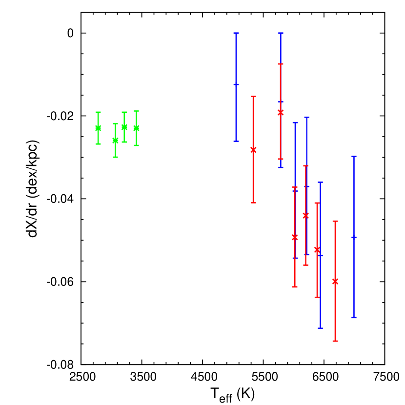
Figure 8: The estimated metallicity gradient $d$[Fe/H]$/dL_{z}$ from the GCS stars (red) and from the RAVE stars (blue) reproduced from Fig. 6. The green points show $d\zeta_{\rm TiO}/dL_{z}$ from the M-dwarf stars in Fig. 7 further subdivided by spectral sub-class. The error bars show 95% confidence limits from Theil’s algorithm.

Furthermore, both samples also hint at a break in the trend with temperature around $T_{\rm eff}$$\;\lesssim 6\,000\;$K, although these points alone are also consistent with a uniform trend. In order to find extra evidence for this possible break of slope, we attempt to include the M-dwarf stars into our analysis.

3.3 M-dwarf sample

Fig. 7 shows the distribution of $L_{z}$ and $\zeta_{\rm TiO}$ for the M-dwarf stars separated into two groups by spectral class. This metallicity indicator again has a noticeable gradient with $L_{z}$.

As for the hotter stars, we have used Theil’s algorithm to estimate the gradient $d\zeta_{\rm TiO}/dL_{z}$, dividing the M-dwarf sample into four groups by stellar sub-class, and plot the results in green in Fig. 8. (The abscissae were determined from the relation $T_{\rm eff}$$\;=3700-150S\;$K, where $S$ is the spectral sub-class, fitted by eye to the compilation by Reylé et al. (2011).) The M-dwarfs have a constant metallicity gradient that appears independent of $T_{\rm eff}$.

Because they are measured from a different quantity, the values of $d\zeta_{\rm TiO}/dL_{z}$ cannot be compared directly with those of $d$[Fe/H]$/dL_{z}$ from the hotter stars, shown in red and blue. We tried using the empirical relation between $\zeta_{\rm TiO}$ and [Fe/H] suggested by Woolf et al. (2009), but many [Fe/H] values required an extrapolation beyond the range calibrated by their study, and the resulting mean [Fe/H] is unreasonably high. Thus we lack a direct basis to relate the green points in Fig. 8 to the others.

However, we note that if $\zeta_{\rm TiO}$ is proportional to [Fe/H], the gradient $d$[Fe/H]$/dL_{z}$ will scale with $d\zeta_{\rm TiO}/dL_{z}$, and we would merely need to shift the green points vertically by some fixed factor to bring them onto the same scale. Since an anti-correlation between $\zeta_{\rm TiO}$ and [Fe/H] seems unlikely, the green points probably could not be shifted above $d$[Fe/H]$/dL_{z}=0$. Thus the data from the M-dwarf stars do seem to confirm that the decreasing trend of metallicity gradient with $T_{\rm eff}$ among the hotter stars really does break to no trend around $T_{\rm eff}$$\;\lesssim 6\,000\;$K, i.e. for stars whose main-sequence lifetimes are $\sim 10^{10}\;$yr.

4 Discussion

Many authors (e.g. Lee et al., 2011; Casagrande et al., 2011; Coşkunoğlu et al., 2011) express concerns that estimates of the metallicity gradient from a sample of stars depend upon the adopted selection criteria. This is because metallicity is a function of age and, relative to younger stars, older stars typically have larger peculiar velocities, which causes an asymmetric drift and greater vertical motion. This well-known kinematic trend must cause an age bias in kinematically selected samples.

4.1 Possible selection effects

In this work, we apply kinematic and vertical motion cuts to eliminate most thick disk and halo stars, which may well also eliminate some old thin disk stars that should perhaps be included in our samples. However, any bias in our analysis created by excluding older stars because of their higher peculiar velocities will cause lower temperature bins, which are the only bins to include stars of the old disk, to have unrepresentatively few older disk stars.

Radial mixing implies that these possibly-missing stars would be members of the most well-mixed population with the lowest radial metallicity gradient, and adding significant numbers of them to the lower $T_{\rm eff}$ bins would only increase the trend we observe. In fact, we find that the trend of metallicity gradient with $T_{\rm eff}$ is little affected by limiting the vertical excursions of selected stars to either 300 pc or 500 pc, suggesting that this cut is not biasing our result. Further restricting the vertical oscillations to $<300\;$pc, on the other hand, does exclude a disproportionate fraction of older stars and the trend with $T_{\rm eff}$ is weakened, as our argument predicts. Naturally also, the number of selected stars decreases with a more severe restriction increasing the statistical uncertainty in our estimate of the metallicity gradient.

We do not use any measure of chemical composition to select stars, and our sample may therefore include some stars with enhanced [$\alpha$/Fe]. Whether such abundances best characterize thick disk stars is the subject of current debate (Ivezić et al., 2008; Lee et al., 2011) while the existence of a thick disk that is distinct from the thin has been questioned (Bovy et al., 2011). Our study is unaffected by these questions, because we are interested only in how the metallicity gradient changes with the mean age of the stars and, provided we have excluded halo stars that are little affected by spiral activity, we do not need to consider whether each star may or may not belong to a particular population. Note that Solway et al. (2012) have shown that mixing is only gradually weakened by increased random motion and vertical thickness.

A separate issue is that all the stars in this study are close to the Sun at the present time, and we therefore cannot include stars with home radii far from the Sun but with radial excursions that are too small to bring them into the solar neighborhood. However, provided the stars we do see have abundances that are representative of those of their $T_{\rm eff}$ and home radius, the omitted stars will not affect our estimate of the slope. Since we are not selecting on metallicity, there should be no bias in our slope estimates.

4.2 Comparison with other work

Casagrande et al. (2011) re-analysed the GCS using a revised calibration of $T_{\rm eff}$ and [Fe/H] and new estimates of the individual stellar ages. We have tried to compare our results with theirs, which is not straightforward because our bins of $T_{\rm eff}$ each contain stars having a broad range of ages. We have used isochrone tables (Demarque et al., 2004) to estimate the main-sequence lifetimes of the individual stars in the GCS sample, using the $T_{\rm eff}$ and [Fe/H] of each, and so find the average main-sequence lifetime of the stars in our separate $T_{\rm eff}$ bins. The mean maximum age of stars defined in this way increases from about 2 Gyr for our hottest bin to 10 Gyr for the coolest. Using these mean maximum ages to replot the trend of metallicity gradient in our Fig. 8, we find reasonable agreement with the gradient values as a cumulative function of age shown in Fig. 18(d) of Casagrande et al. (2011).

Our estimated gradient is in the range of other measurements from stars. For example, Coşkunoğlu et al. (2011) derived a metallicity gradient of -0.051 dex kpc^-1 for F-dwarfs, and they also find a shallower gradient for the slightly older G-dwarfs. While their sample clearly overlaps with ours, they adopted different selection criteria and employed a different technique to determine the home radii, it is encouraging that they reached similar conclusions. Using disk Cepheids, which are young objects, Luck et al. (2011) derived [Fe/H]$=-0.055R+0.475$, where $R$ is the Galacto-centric radius, again in tolerable agreement with our gradient estimate for the hotter stars.

Chen et al. (2003) estimate a radial gradient of [Fe/H] of $-0.063\pm 0.008$ dex kpc^-1 from 118 star clusters. Both they and Friel et al. (2002) report that, when the clusters are divided by age, the slope appears steeper for the older sample, which is the opposite of our finding here. Note that the radial distribution of star clusters in these papers extends outwards from the solar radius, whereas our sample of stars overlaps the solar radius and extends inwards to $\sim 5\;$kpc – thus the different variations with age could indicate the absence of mixing in the outer disk. However, other systematic differences may complicate this interpretation; e.g., the outer disk open clusters in the sample assembled by Chen et al. (2003) are farther from the mid-plane than are those near the solar radius.

Maciel et al. (2006) also claim a steeper abundance gradient for older planetary nebulae, although their estimated gradients for the different elements show a lot of scatter and ages are less reliable than for star clusters. It should be noted that Stanghellini & Haywood (2010) reached the opposite conclusion finding, for a sample of PNe concentrated over the radial range $3<R<12\;$kpc, a shallower abundance gradient for the older PNe, which is in better agreement with our results.

5 Conclusions

We have used samples of local thin-disk, main-sequence stars grouped by effective temperature to demonstrate that the radial abundance gradient in the disk of the Milky Way flattens as the $T_{\rm eff}$ of the stars in the sample decreases. We eliminate the blurring effect of epicyclic motion by estimating the angular momentum, $L_{z}$, of each star about the center of the Galaxy, since the home, or guiding center, radius of a star is determined only by its angular momentum. Although the stars in our sample are all within 500 pc of the Sun, their home radii are spread over a wide swath of the Milky Way disk.

We interpret $T_{\rm eff}$ as a proxy for mean age, and conclude that a shallower gradient for stars of a greater mean age. We find some evidence that the trend of decreasing metallicity gradient with increasing age breaks to a flat trend around $5\,500\lesssim\hbox{{$T_{\rm eff}$}}\lesssim 6\,000\;$K, for which the main-sequence lifetime of a star is approximately 10 Gyr, or roughly the age of the thin disk. Flattening of the metallicity gradient is consistent with the predictions of radial mixing, or churning, due to spiral patterns in the disk.

References

- (1)
- Aumer & Binney (2009) Aumer, M. & Binney, J. J. 2009, MNRAS, 397, 1286
- Balser et al. (2011) Balser, D. S., Rood, R. T., Bania, T. M. & Anderson, L. D. 2011, ApJ, 738, 27
- Bensby et al. (2003) Bensby, T., Feltzing, S. & Lundström, I. 2003, A&A, 410, 527
- Binney & Tremaine (2008) Binney, J. & Tremaine, S. 2008, Galactic Dynamics 2nd Ed. (Princeton: Princeton University Press)
- Bird et al. (2012) Bird, J. C., Kazantzidis, S. & Weinberg, D. H. 2012, MNRAS, 420, 913
- Breddels et al. (2010) Breddels, M. A., Smith, M. C., Helmi, A., et al. 2010, A&A, 511, A90
- Boissier & Prantzos (1999) Boissier, S. & Prantzos, N. 1999, MNRAS, 307, 857
- Bovy et al. (2011) Bovy, J., Rix, H-W. & Hogg, D. W. 2011, arXiv:1111.6585
- Casagrande et al. (2011) Casagrande, L., Schönrich, R., Asplund, M., et al. 2011, A&A, 530, A138
- Chen et al. (2003) Chen, L., Hou, J. L. & Wang, J. J. 2003, AJ, 125, 1397
- Chiappini et al. (2001) Chiappini, C., Matteucci, F. & Romano, D. 2001, ApJ, 554, 1044
- Coşkunoğlu et al. (2011) Coşkunoğlu, B., Ak, S., Bilir, S., et al. 2011, MNRAS, in press
- de Jong (1999) de Jong, R. S. 1996, A&A, 313, 377
- Demarque et al. (2004) Demarque, P., Woo, J-H., Kim, Y-C. & Yi, S. K. 2004, ApJS, 155, 667
- Edvardsson et al. (1993) Edvardsson, B., Andersen, B., Gustafsson, B., et al. 1993, A&A, 275, 101
- Friel et al. (2002) Friel, E. D., Janes, K. A., Tavarez, M., et al. 2002, AJ, 124, 2693
- Fu et al. (2009) Fu, J., Hou, J. L., Yin, J. & Chang, R. X. 2009, ApJ, 696, 668
- Haywood (2008) Haywood, M. 2008, MNRAS, 388, 1175
- Hou et al. (2000) Hou, J. L., Prantzos, N. & Boissier, S. 2000, A&A, 362, 921
- Girard et al. (2011) Girard, T. M., van Altena, W. F., Zacharias, N., et al. 2011, AJ, 142, 15
- Høg et al. (2000) Høg, E., Fabricius, C., Makarov, V. V., et al. 2000, A&A, 355, L27
- Hollander & Wolfe (1999) Hollander, M. & Wolfe, D. A. 1999, Nonparametric Statistical Methods 2nd Ed. (New York: John Wiley) pp. 416–423
- Holmberg et al. (2007) Holmberg, J., Nordström, B. & Andersen, J. 2007, A&A, 475, 519
- Holmberg et al. (2009) Holmberg, J., Nordström, B. & Andersen, J. 2009, A&A, 501, 941
- Ivezić et al. (2008) Ivezić, Z̆., Sesar, B., Jurić, M., et al. 2008, ApJ, 684, 287
- Johnson & Soderblom (1987) Johnson, D. R. H. & Soderblom, D. R. 1987, AJ, 93, 864
- Lee et al. (2008) Lee, Y. S., Beers, T. C., Sivarani, T., et al. 2008, AJ, 136, 2022
- Lee et al. (2011) Lee, Y. S., Beers, T. C., An, D., et al. 2011, ApJ, 738, 187
- Loebman et al. (2011) Loebman, S. R., Ros̆kar, R., Debattista, V. P., et al. 2011, ApJ, 737, 8
- Luck et al. (2011) Luck, R. E., Andrievsky, S. M., Kovtyukh, V. V., et al. 2011, AJ, 142, 51
- Maciel et al. (2006) Maciel, W. J., Lago, L. G. & Costa, R. D. D. 2006, A&A, 453, 587
- Maciel et al. (2007) Maciel, W. J., Quireza, C. & Costa, R. D. D. 2007, A&A, 463, L13
- Minchev et al. (2011) Minchev, I., Famaey, B., Combes, F., et al. 2011, A&A, 527A, 147
- Muñoz-Mateos et al. (2007) Muñoz-Mateos, J. C., Gil de Paz, A., Boissier, S., 2007, ApJ, 658, 1006
- Munn et al. (2004) Munn, J. A., Monet, D. G., Levine, S. E., et al. 2004, AJ, 127, 3034
- Munn et al. (2008) Munn, J. A., Monet, D. G., Levine, S. E., et al. 2008, AJ, 136, 895
- Naab & Ostriker (2006) Naab, T. & Ostriker, J. P. 2006, MNRAS, 366, 899
- Nordström et al. (2004) Nordström, B., Mayor, M., Andersen, J., et al. 2004, A&A, 418, 989
- Piatek et al. (2002) Piatek, S., Pryor, C., Olszewski, E. W., et al. 2002, AJ, 124, 3198
- Reid et al. (2007) Reid, I. N., Turner, E. L., Turnbull, M. C., et al. 2007, ApJ, 665, 767
- Reylé et al. (2011) Reylé, C., Rajpurohit,, A. S., Schultheis, M. & Allard, F. 2011, arXiv:1102.1263
- Ros̆kar et al. (2008a) Ros̆kar, R., Debattista, V. P., Quinn, T. R., et al. 2008a, ApJL, 684, L79
- Ros̆kar et al. (2008b) Ros̆kar, R., Debattista, V. P., Stinson, G. S., et al. 2008b, ApJL, 675, L65
- Schlesinger et al. (2011) Schlesinger, K. J., Johnson, J. A., Rockosi, C. M., et al. 2011, ApJ, submitted (arXiv:1112.2214)
- Schönrich & Binney (2009) Schönrich, R. & Binney, J. 2009, MNRAS, 396, 203
- Schönrich et al. (2010) Schönrich, R., Binney, J. & Dehnen, W. 2010, MNRAS, 403, 829
- Sellwood & Binney (2002) Sellwood, J. A. & Binney, J. J. 2002, MNRAS, 336, 785
- Shaver et al. (1983) Shaver, P. A., McGee, R. X., Newton, L. M., 1983, MNRAS, 204, 53
- Siebert et al. (2011) Siebert, A., Williams, M. E. K., Siviero, A., et al. 2011, AJ, 141, 187
- Soderblom (2010) Soderblom, D. R. 2010, ARAA, 48, 581
- Solway et al. (2012) Solway, M., Sellwood, J. A. & Schönrich, R. 2010, MNRAS, to appear (arXiv:1202.1418)
- Stanghellini & Haywood (2010) Stanghellini, L. & Haywood, M. 2010, ApJ, 714, 1096
- Steinmetz et al. (2006) Steinmetz, M., Zwitter, T., Siebert, A., et al. 2006, AJ, 132, 1645
- van Leeuwen (2007) van Leeuwen, F. 2007, A&A, 474, 653
- West et al. (2011) West, A. A., Morgan, D. P., Bochanski, J. J., et al. 2011, AJ, 141, 97
- Woolf et al. (2009) Woolf, V. M., Lépine, S. & Wallerstein, G. 2009, PASP, 121, 117
- Wielen (1977) Wielen, R. 1977, A&A, 60, 263
- Yanny et al. (2009) Yanny, B., Rockosi, C., Newberg, H. J., et al. 2009, AJ, 137, 4377
- York et al. (2000) York, D. G., Adelman, J., Anderson, J. E., et al. 2000, AJ, 120, 1579
- Zwitter et al. (2008) Zwitter, T., Siebert, A., Munari, U., et al. 2008, AJ, 136, 421
- Zwitter et al. (2010) Zwitter, T., Matijevic̆, G., Breddels, M. A., et al. 2010, A&A, 522, A54