An epidemic process mediated by a decaying diffusing signal

Abstract

We study a stochastic epidemic model consisting of elements (organisms in a community or cells in tissue) with fixed positions, in which damage or disease is transmitted by diffusing agents (“signals”) emitted by infected individuals. The signals decay as well as diffuse; since they are assumed to be produced in large numbers, the signal concentration is treated deterministically. The model, which includes four cellular states (susceptible, transformed, depleted, and removed), admits various interpretations: spread of an infection or infectious disease, or of damage in a tissue in which injured cells may themselves provoke further damage, and as a description of the so-called radiation-induced bystander effect, in which the signals are molecules capable of inducing cell damage and/or death in unirradiated cells. The model exhibits a continuous phase transition between spreading and nonspreading phases. We formulate two mean-field theory (MFT) descriptions of the model, one of which ignores correlations between the cellular state and the signal concentration, and another that treats such correlations in an approximate manner. Monte Carlo simulations of the spread of infection on the square lattice yield values for the critical exponents and the fractal dimension consistent with the dynamic percolation universality class.

I Introduction

In many epidemic-like processes disease spreads via an agent emitted by the affected elements (cells or organisms) themselves Mollis . Epidemics have been modeled extensively using deterministic reaction-diffusion equations murray , and stochastic particle systems grass1 ; cardy ; Linder ; Souza . In the simplest epidemic models, such as the susceptible-infected-removed (SIR) and susceptible-infected-removed-susceptible (SIRS) processes Bartlett , disease is transmitted by contact between infected and healthy organisms, without explicit representation of a transmitting agent. But since the latter may have a dynamics of its own, typically involving diffusion and decay, it is of interest to include this agent explicitly in a more complete description, particularly when the spatial structure of the epidemic is analyzed.

A similar observation applies to a viral infection, and to the spread of damage in tissue following irradiation. In the latter case, initially affected cells may become sources of a signal that damages nearby cells, which were not harmed in the initial event. These secondary cells may then become additional sources of the harmful signal. Such a scenario has been proposed for the radiation-induced bystander effect (RIBE) BSDM ; Mothersill97 ; Mothersill98 . While the direct result is damage to some or all of the irradiated cells, the long-term effect is characterized by damage or death of unirradiated cells or “bystanders”. It is thought that irradiated cells release a signal (possibly a cytokine) that diffuses through the medium, causing damage in previously healthy, unirradiated cells BSDM . Thus signal molecules in RIBE play a role analogous to a disease agent in an epidemic.

In this work we introduce an epidemic model in which damaged or infected elements briefly emit signals; the latter diffuse and decay at a certain rates. Healthy organisms or cells may become infected or damaged due to the presence of the signal, and so may become new sources. We formulate the model on a discrete two-dimensional space, the square lattice.

Epidemic models with spatial structure and short-range interactions have been studied intensively in recent years bai ; grass1 ; Souza ; sat1 ; sat2 ; Tome-Ziff , and applied to the spread of disease in humans and plants kuu ; sander ; gonci . Here we focus on processes initiated in a single cell or organism, or in a localized region. Key questions are then (1) the rate of spreading, as reflected in the growth in the number of affected individuals, and their spatial distribution, and (2) whether spreading continues indefinitely, limited only by the size of the available region, or stops before attaining a size comparable to the of the system. In the infinite system-size limit, the two regimes are separated by a phase transition. In the supercritical (spreading) phase, there is a nonzero probability to spread indefinitely, whereas in the subcritical (nonspreading) phase the process dies out with probability one.

Phase transitions in stochastic epidemic models with spatial structure have received considerable attention; an important example is the general epidemic process (GEP) Mollis ; grass1 . The GEP is essentially a stochastic susceptible-infected-removed (SIR) model with spatial structure. Initially, all individuals are susceptible (S) except for one or a few infecteds (I). Susceptibles with one or more I neighbors become infected at a certain rate $\lambda$, while infecteds recover at rate $\mu$, after which they are forever immune, hence removed (R) from interactions with other individuals. Transmission (S+I $\to$ 2I) is typically restricted to nearest-neighbor S-I pairs on a regular lattice or a network. The GEP exhibits a phase transition as the ratio $\lambda/\mu$ is varied. The supercritical phase is characterized by a growing active region, which invades regions containing susceptibles and leaves behind an inactive region composed of individuals in states S and R. Activity is thus restricted to a “ring” separating as yet unaffected and formerly active regions. (In a finite system, the final state is completely inactive.) Analysis of the GEP shows that its critical behavior belongs to the dynamic percolation universality class grass1 ; Tome-Ziff . If the process is modified so that a recovered individual can become susceptible (SIRS model), it is possible to maintain an active stationary state in which the processes of infection, recovery, and loss of immunity occur continuously. The SIRS model with spatial structure exhibits a phase transition belonging to the directed percolation (DP) universality class Henkel ; Souza , exemplified by the contact process harris ; marro .

In this work we study a model in which individuals may be in one of four states: susceptible (S), transformed (T), depleted (D), and removed (R), the latter class designating individuals that have died or are otherwise sequestered from the rest of the population. The principal new feature of our model is the mechanism by which infection is transmitted: the transition from susceptible to transformed is mediated by a signal released by cells in state T, rather than via direct contact. Such cells may recover (becoming susceptible once again), may be removed, or may emit signals. In the latter case, the cell immediately enters state D, after which it may either recover or be removed. Although cells in states T or D may recover, there is a finite probability of permanent removal. Thus we expect that, as in the GEP, the process will exhibit spreading and nonspreading phases, with activity concentrated in a ring. Assuming the phase transition is continuous, it is reasonable to expect the critical behavior to be that of dynamic percolation. Given the novel mode of transmission, it is nonetheless of interest to verify this assumption.

The remainder of this paper is organized as follows. We define the model in Sec. II, and in Sec. III discuss two mean-field approaches, a simple one that ignores diffusion, and a more detailed formulation that takes diffusion into account while still assuming spatial homogeneity. In Sec. IV we present simulation results for the phase diagram, critical behavior, cluster properties, and spreading velocity. A summary and a discussion of our results are provided in Sec. V.

II Model

The model is defined on a square lattice of $L^{2}$ sites, each of which hosts an individual (an organism or a cell, depending on the choice of interpretation). Individuals exist in one of four states: susceptible (S), transformed (T), depleted (D), or removed (R). In addition to the discrete state variable, each site $(i,j)$ bears a signal concentration $C_{ij}\geq 0$. Individuals emit signals upon making the transition from state T to state D; we adopt concentration units such that each such event produces one unit of signal molecules. The transitions between states are as follows:

(i) An individual in state S, at site $(i,j)$, has transition rates $\mu C_{ij}$ and $\nu C_{ij}$ to states T and R, respectively. These are the only rates that depend on the signal concentration.

(ii) An individual in state T has transition rates $w_{TS}$, $w_{TD}$ and $w_{TR}$, to states S, D and R, respectively.

(iii) An individual in state D has transition rates $w_{DS}$ and $w_{DR}$, to states S and R, respectively.
The states and transitions are summarized in Fig. 1; note that state R allows no escape.

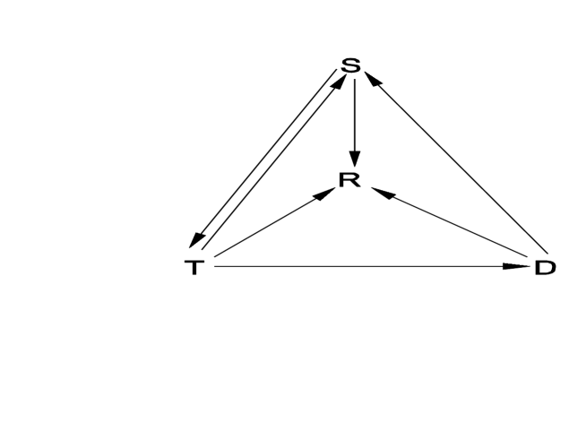
Figure 1: States and allowed transitions. The rates for transitions out of state S are proportional to the local concentration of signal. The latter is produced when individuals move from state T to state D.

The signal concentration $C_{ij}(t)$ evolves via diffusion and decay. We assume that the number of signal molecules is very large, so that the concentration may be treated deterministically, via the equation

$$\frac{dC_{ij}}{dt}={\cal D}\Delta C_{ij}-\lambda C_{ij}+\sum_{k=1}^{n_{ij}}\delta(t-t_{k;ij}),$$ (1)

where $\Delta$ denotes the discrete Laplacian, $D$ is the diffusion rate, $\lambda$ is the decay rate, $n_{ij}$ is the number of times site $(i,j)$ has made the transition from T to D, and the $t_{k;ij}$ are the transition times. Since the $n_{i,j}$ and the transition times are random variables, the $C_{i,j}$ are as well.

In the limit of very low signal concentration, the discrete nature of the signal molecules makes an important contribution to the fluctuations. Thus our continuum, deterministic description may not be suitable for the low-concentration limit. Another possibly troublesome aspect of the diffusion equation is that, given a localized source at time zero, the concentration at any time $t>0$ is nonzero (albeit very small) at points arbitrarily far from the source. While this is unphysical, we do not expect it to cause any significant effect in the system under study. Indeed, the diffusion equation is widely applied, with apparent success, in modeling biological transport, and systems of reaction-diffusion equations (including appropriate noise terms) have been found to yield reliable predictions for critical properties of nonequilibrium systems Henkel .

The model involves a rather larger set of parameters: the coefficients $\mu$ and $\nu$, the diffusion and decay rates, and five additional transition rates. It is nevertheless clear that large values of $\mu$ and $w_{TD}/(w_{TR}+w_{TS})$, and small values of $\lambda$, favor spreading. Evidently, spreading can only occur for ${\cal D}>0$. Note that for $w_{DS}=0$, there is no functional difference between states D and R, and we have a simpler, three-state model.

We are primarily interested in an initial condition consisting of the origin in state D, with an associated unitary signal concentration, and with all other sites in state S, and free of any signal. The ensuing evolution corresponds to an epidemic spreading from the origin. The current size of an epidemic can be defined as the number of individuals in states other than S. Of particular interest are the number $N_{R}(t)$ of removed individuals, the number $N_{T}(t)$ of individuals in state T, and the (spatial) average signal concentration, $C(t)$. The latter two quantities reflect the degree of spreading activity, since, if both are zero, further advance of the epidemic is impossible. In the spreading phase, starting from a small, localized set of affected individuals, $N_{R}$ and $C$ grow without limit in an unbounded system, whereas in the nonspreading phase these quantities cease to grow after a certain time. In a finite system, $N_{R}$ and $C$, must eventually saturate, even in the spreading phase. The distinction between spreading and nonspreading phases is nonetheless evident in large, finite systems since, in the spreading phase, a finite fraction of individuals are eventually affected, whereas in the nonspreading phase the final fraction of affected individuals is $\sim 1/L^{2}$ ker ; daley . It is worth noting that, strictly speaking, an absorbing configuration corresponds to one without transformed cells, and with the signal concentration everywhere zero. Since $C$ decays at a finite rate, such a situation can only obtain in the infinite-time limit. The implications for defining survival are discussed in Sec. IV.

For simplicity, we assume that the signal-dependent transitions (i.e., from S to either T or R) have rates that are proportional to the local signal concentration. Other dependencies are conceivable; at the end of the next section we briefly consider rates proportional to $C^{2}$.

III Mean-field analysis

In the simplest mean-field analysis we factorize the joint probability distribution for the $N$-site system into a product of single site probabilities, and treat the signal concentration $C_{ij}$ as independent of the state of the site. Denoting the probabilities for site ($i,j$) to be in state S, T, D, or R by $S_{ij}$, $T_{ij}$, $D_{ij}$, and $R_{ij}$ respectively, and the mean signal concentration by $C_{ij}$, we then have:

$$\frac{dC_{ij}}{dt} = {\cal D}\sum_{\langle kl,ij\rangle}(C_{kl}-C_{ij})+w_{TD}T_{ij}-\lambda C_{ij}$$ (2)

$$\frac{dS_{ij}}{dt} = -(\mu+\nu)C_{ij}S_{ij}+w_{TS}T_{ij}+w_{DS}D_{ij}$$ (3)

$$\frac{dT_{ij}}{dt} = \mu C_{ij}S_{ij}-(w_{TS}+w_{TD}+w_{TR})T_{ij}$$ (4)

$$\frac{dD_{ij}}{dt} = w_{TD}T_{ij}-(w_{DS}+w_{DR})D_{ij}$$ (5)

$$\frac{dR_{ij}}{dt} = \nu C_{ij}S_{ij}+w_{TR}T_{ij}+w_{DR}D_{ij}$$ (6)

where the sum in the first equation extends over the nearest neighbor sites ($k,l$) of site ($i,j$). If we take the continuum limit of these equations and let ${\bf X}({\bf r})\equiv(C,S,T,D,R)$, we obtain a set of reaction-diffusion equations, $\partial{\bf X}/{\partial t}={\sf D}\nabla^{2}{\bf X}+{\bf f}({\bf X})$, in which only the element $D_{cc}$ of the diffusion matrix is nonzero.

We study a spatially uniform mean-field theory, which corresponds to the fast-diffusion limit. In this case the MF equations for the site probabilities are as above (removing the subscripts $ij$ on all variables), while the concentration satisfies

$$\frac{dC}{dt}=wT-\lambda C$$ (7)

Given the large set of parameters, it is convenient to fix all but one, which then plays the role of a control parameter. Somewhat arbitrarily, we choose $w\equiv w_{TD}$ (i.e., the rate at which transformed cells emit signal and become depleted), as the control parameter, and denote its critical value by $w_{c}$. We use the uniform analysis to set basic limits on survival of the spreading process, by studying an epidemic scenario. That is, we consider a very small initial source probability $D(0)$, $S(0)=1-D(0)\simeq 1$, and $T(0)=R(0)=0$. (We set $D(0)=C(0)=10^{-13}$.) Then, as $t\to\infty$, a non-vanishing value of $R$ corresponds to an epidemic in which a nonzero fraction of individuals are affected, i.e., to the spreading phase.

Figure 2 shows the evolution of the transformed fraction $T(t)$; in the nonspreading phase $T(t)$ decays monotonically, while in the spreading phase it grows at intermediate times. The depleted fraction $D(t)$ exhibits a similar behavior. The fraction of removed individuals, $R(t)$, grows steadily in the spreading regime, until it saturates; in the nonspreading regime it saturates at a very small value (see Fig. 3). In the spreading phase, the growth regime is followed by a crossover to exponential decay, marking the end of the epidemic. The crossover occurs due to the depletion of susceptibles.

A simple analysis allows us to determine the boundary between spreading and nonspreading phases. Since we are interested in the early stage of the evolution (following the initial transient) we set $S=1$, and seek a solution in which the probabilities $T$ and $D$, and the signal concentration grow exponentially: $T(t)=T_{1}e^{\gamma t}$, and similarly for $D$ and $C$. Inserting these expressions in the MF equations yields

$$(\gamma+\lambda)(\gamma+w_{T})=\mu w$$ (8)

where $w_{T}=w+w_{TS}+w_{TR}$. Equating $\gamma$ to zero yields the critical threshold:

$$w_{c}=\frac{\lambda(w_{TR}+w_{TS})}{\mu-\lambda}$$ (9)

Note that spreading is impossible for $\mu<\lambda$, and that $w_{c}$ is independent of parameters $\nu$, $w_{DS}$ and $w_{DR}$. The above conclusions are verified in numerical solutions of the (uniform) MF equations.

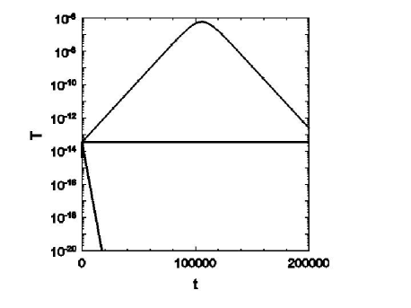
Figure 2: Transformed fraction $T(t)$ in uniform mean-field theory. Parameters $\lambda=0.05$, $\mu=0.2$, $\nu=0.1$, $w_{TR}=w_{DR}=w_{TS}=w_{DS}=0.2$, and (lower to upper) $w=0.13$, $0.13333...=w_{c}$, and $0.134$.

Figure 3: Uniform mean-field theory: limiting fraction of removed individuals versus $w$.

The original MF equations, Eq. (6), not only treat sites as independent, but also treat the concentration at a site as independent of its state. This is a rather drastic approximation, because signal molecules are only created when a site undergoes the transition T $\to$ D; other sites only acquire a nonzero signal concentration via diffusion. This approximation can be improved by introducing a concentration variable $C_{J}$ for each site type; here $C_{J}$ denotes the mean concentration at a site, given that it is in state $J$. To derive a set of mean-field equations for the site probabilities and the associated concentrations, we treat the amount of signal at a given site as a discrete variable, $n$. Let $P(J,n,t)$ denote the (joint) probability that a site is in state J and has exactly $n$ units of signal. Then the probability of state $J$ is $P(J,t)=\sum_{n}P(J,n,t)$, and $C_{J}(t)=\sum_{n}nP(J,n,t)/\sum_{n}P(J,n,t)=\sum_{n}nP(J,n,t)/P(J,t)$, so that

$$\frac{dC_{J}}{dt}=\frac{\sum_{n}n[dP(J,n,t)/dt]}{P(J,t)}-\frac{[dP(J,t)/dt]C_{J}(t)}{P(J,t)}$$ (10)

Consider, for example, state S. There are contributions to $dP(S,n,t)/dt$ due to (1) decay of the signal; (2) diffusion between the site and its neighbors; and (3) transitions between state S and other states. To treat diffusion at this level of approximation, we suppose that all four neighbors of a given site have the same, average concentration, $\overline{C(t)}=\sum_{J}P(J,t)C_{J}(t)$. Then we have

$$\frac{dP(S,n,t)}{dt} = \lambda[(n+1)P(S,n+1,t)-nP(S,n,t)]$$ (11)

$$+ 4D\overline{C}[P(S,n-1,t)-P(S,n,t)]+4D[(n+1)P(S,n+1,t)-nP(S,n,t)]$$

$$+ w_{TS}P(T,n,t)+w_{DS}P(D,n,t)-n(\mu+\nu)P(S,n,t).$$

Summing over $n$, we find,

$$\frac{\sum_{n}n[dP(S,n,t)/dt]}{P(S,t)} = -\lambda C_{S}+4{\cal D}[\overline{C}-C_{S}]-(\mu+\nu)\langle n^{2}\rangle_{S}$$ (12)

$$+ w_{TS}C_{T}\frac{P(T)}{P(S)}+w_{DS}C_{D}\frac{P(D)}{P(S)},$$

where $\langle n^{2}\rangle_{S}\equiv\sum_{n}n^{2}P(S,n.t)/P(S,t)$. The second term in Eq. (10) involves,

$$\frac{\sum_{n}[dP(S,n,t)/dt]}{P(S,t)}=-(\mu+\nu)C_{S}+w_{TS}\frac{P(T)}{P(S)}+w_{DS}C_{D}\frac{P(D)}{P(S)}.$$ (13)

Multiplying by $C_{S}$ and subtracting the result from Eq. (12), we obtain

$$\frac{dC_{S}}{dt}=-\lambda C_{S}+4{\cal D}[\overline{C}-C_{S}]+w_{TS}[C_{T}-C_{S}]\frac{P(T)}{P(S)}+w_{DS}[C_{D}-C_{S}]\frac{P(D)}{P(S)},$$ (14)

where we have set var$(n)=\langle n^{2}\rangle_{S}-C_{s}^{2}$ to zero, as is usual in a mean-field approach. Proceeding in the same manner, we find,

$$\frac{dC_{T}}{dt}=-\lambda C_{T}+4{\cal D}[\overline{C}-C_{T}]+\mu C_{S}[C_{S}-C_{T}]\frac{P(S)}{P(T)},$$ (15)

$$\frac{dC_{D}}{dt}=-\lambda C_{D}+4{\cal D}[\overline{C}-C_{D}]+w[1+C_{T}-C_{D}]\frac{P(T)}{P(D)},$$ (16)

and

$$\frac{dC_{R}}{dt} = -\lambda C_{R}+4{\cal D}[\overline{C}-C_{R}]+\nu C_{S}[C_{S}-C_{R}]\frac{P(S)}{P(R)}$$ (17)

$$+ w_{TR}[C_{T}-C_{R}]\frac{P(T)}{P(R)}+w_{DR}[C_{D}-C_{R}]\frac{P(D)}{P(R)}.$$

Numerical solution of this set of equations yields a critical threshold, $w_{c}$, which decreases monotonically with diffusion rate ${\cal D}$, approaching the value of the simple MF analysis as ${\cal D}\to\infty$. Figure 4 shows the evolution of the state probabilities and concentrations in a near-critical system, as predicted by the diffusive mean-field theory (DMFT). The predictions of DMFT for $w_{c}$ are compared with simulation results in the following section.

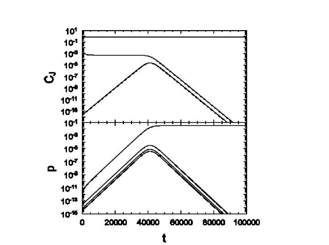
Figure 4: Diffusive mean-field theory: temporal evolution. Lower panel (lower to upper): state probabilities $P(D,t)$, $P(T,t)$, total signal concentration $C(t)$, and $P(R,t)$; upper panel (lower to upper): conditional concentrations $C_{S}$ and $C_{T}$ (indistinguishable at this scale), $C_{R}$, and $C_{D}$. Parameters $\lambda=0.05$, $\mu=0.2$, $\nu=0.1$, $w_{TR}=w_{DR}=w_{TS}=w_{DS}=0.2$, ${\cal D}=0.02$, and $w=0.2$, slightly greater than $w_{c}=0.19587$.

An advantage of MFT is that it readily allows investigation of diverse scenarios. We use MFT to perform a preliminary study of a variant of the model defined above, in which the rates for the transitions S $\to$ T and S $\to$ R are $\mu C^{2}$ and $\nu C^{2}$, respectively, representing a situation in which healthy individuals are essentially insensitive to very low signal concentrations. In the epidemic context, this corresponds to a situation in which small concentrations of a disease agent are effectively eliminated by the immune system, whereas higher concentrations overwhelm it. Experience with nonequilibrium phase transitions in systems such as Schlögl’s second model schlogl , leads one to expect a discontinuous phase transition in this case. This is indeed verified for certain sets of parameters, featuring relatively large values of $\mu$; an example is shown in Fig. 5. (Note that in this case the transition value $w_{c}$ depends on the initial signal concentration.)

Figure 5: MFT: Final removal fraction $R_{\infty}$ versus $w$ for $\mu=10$, $C(0)=0.01$, when the transition rates from S to T and S to R are $\propto C^{2}$, with other parameters as in Fig. 2. $R_{\infty}$ jumps from about 0.16 to 0.998 when $w=0.15335$.

IV Simulations

Simulations of the model defined in Sec. II are performed on square lattices of $L\times L$ sites. These studies begin with all sites in state S (and having signal concentration zero) except for the origin, which is in state D, with a signal concentration of unity. Although the boundaries are open, the system size is chosen such that sites on the boundary remain in state S, and have negligible signal concentration, for the duration of the studies. In the simulation algorithm, at each step, corresponding to a time interval $\Delta t$, the cellular states evolve as follows:

(i) if site $(i,j)$ is in state S, it remains in that state with probability $p_{s}=\exp[-(\mu+\nu)C_{ij}\Delta t]$. It makes a transition to state T with probability $(1-p_{s})\mu/(\mu+\nu)$, and to R with probability $(1-p_{s})\nu/(\mu+\nu)$.

(ii) if the site is in state T, it remains in this state with probability $p_{t}=\exp[-w_{T}\Delta t]$. The probability of a transition to state $J$ (=S, D, or R) is $(1-p_{t})w_{TJ}/w_{T}$.

(iii) if the site is in state D, it remains so with probability $p_{d}=\exp[-w_{D}\Delta t]$. The probability of a transition to state J (=S or R) is $(1-p_{d})w_{DJ}/w_{D}$.

(iv) sites in state R remain in this state.

In addition, the signal concentration is updated in accord with Eq. (1), that is, $C_{ij}\to C_{ij}^{\prime}=\exp(-\lambda\Delta t)C_{ij}+{\cal D}\Delta t\sum_{kl}[C_{kl}-C_{ij}]$, with the additional contribution $C_{ij}\to C_{ij}+1$ at a step in which site $(i,j)$ makes a transition from state T to state D. Most of the studies reported below use $\Delta t=0.4$. We found that the results using a smaller time step ($\Delta t=0.2$) we essentially the same. In studies of large ${\cal D}$ values, however, it was necessary to reduce the time step to 0.2 or 0.1 to maintain reliability.

Since the transition between spreading and nonspreading phases is apparently continuous, we determine the critical point $w_{c}$ by searching for power-law behavior of the level of activity $n(t)$, the survival probability $P(t)$, and the mean-square distance of removed cells cells from the origin, $R^{2}(t)$, as functions of time. The activity level $n(t)$ is conveniently defined as the number $N_{T}$ of sites in state T, since growth of the active region requires transformed cells or a nonzero signal concentration. We find that at long times, the behavior of the total signal concentration is similar to that of $N_{T}$.

As noted in Sec. II, the definition of survival is not completely obvious in the present model. Our definition is based on the continued increase in the number of R cells. To begin, we study the distribution of waiting times $t_{w}$ between successive events in which $N_{R}\to N_{R}+1$. Studying a large number of realizations up to some maximum time, $t_{M}$, we find that they can be divided into two classes: those in which $N_{R}$ increases until the end, and those in which this number saturates well before. In the latter class, the final configuration is devoid of T cells, and the total signal concentration is extremely small, so that further growth in $N_{R}$ is essentially impossible. We find that in the class of realizations with sustained activity, the probability distribution of waiting times, $P(t_{w})$, falls to zero above a certain value. On this basis, we define a maximum waiting time time, $t_{WM}$, somewhat larger than the value associated with the cutoff of $P(t_{w})$. If, in a given realization, the waiting time $t_{w}$ exceeds $t_{WM}$, the system is taken to be inactive, and the realization ends; the time of deactivation is taken as that of the most recent transition to state R. The survival probability $P(t)$ is then defined as the fraction of realizations that are active at time $t$. (For the parameter set analyzed below, we use $t_{WM}=180$.)

The quantities $P(t)$, $n(t)$, and $R^{2}(t)$ are expected to follow grass1 ; grass2 ,

$$n(t) \sim t^{\theta},$$ (18)

$$P(t) \sim t^{-\delta},$$ (19)

$$R^{2}(t) \sim t^{z_{sp}},$$ (20)

at the critical point, where $\theta$, $\delta$ and $z_{sp}$ are critical exponents associated with spreading. We expect the cluster generated by the critical process to be a fractal; its radius of gyration should follow $R_{g}\sim n^{1/D_{f}}$, where $D_{f}$ is the fractal dimension stauf .

We perform detailed studies using the parameter values $\lambda=0.05$, $\mu=0.5$, $\nu=0.1$, and $w_{TR}=w_{DR}=w_{TS}=w_{DS}=0.2$, using system sizes $L$ of up to 600, and simulation times of up to $t_{M}=10\,000$ time units. (The number of simulation steps is $t_{M}/\Delta t$.) For each value of the diffusion rate ${\cal D}$ studied, we determine the critical value $w_{c}$ using the power-law criterion for $P(t)$. Specifically, we estimated $w_{c}$ using the local slope $\theta(t)$, as described below. The uncertainty in $w_{c}$, on the order of $5\times 10^{-4}$, reflects the range of $w$ values for which we cannot rule out an asymptotic linear behavior of $\theta(t)$ versus $1/t$ at long times. The resulting phase boundary is compared against mean-field theory in Fig. 6. Mean-field theory furnishes the correct order of magnitude, but underestimates $w_{c}$, especially for small values of ${\cal D}$. The diffusive MFT furnishes a slight improvement over simple MFT. For ${\cal D}\to\infty$, the mean-field prediction converges to 2/45 = 0.0444…; simulations in this limit (using a spatially uniform signal concentration) yield $w_{c}=0.045(1)$, consistent with MFT. Figure 7 shows a similar comparison for $w_{c}$ as a function of $\mu$, for ${\cal D}=0.02$; in this case the DMFT prediction is about a factor of five smaller than the simulation value.

We also determined $w_{c}$ for a rather different set of parameters: $\nu=0.51$, $\mu=0.79$, $\lambda=0.1$, ${\cal D}=2.94$, and $w_{DR}=w_{DS}=w_{TR}=w_{TS}=0.0079$. In this case simulation yields $w_{c}=3.15(5)\times 10^{-3}$, while simple and diffusive MFT yield $w_{c}=2.29\times 10^{-3}$ and $2.31\times 10^{-3}$, respectively. The closer agreement between simulation and MFT in this case can be attributed to the higher diffusion rate.

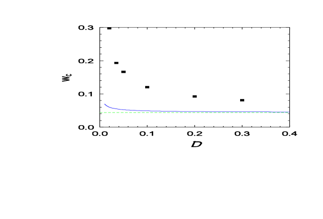
Figure 6: (Color online) Critical rate $w_{c}$ versus diffusion rate ${\cal D}$ for $\lambda=0.05$, $\mu=0.5$, $\nu=0.1$, and $w_{TR}=w_{DR}=w_{TS}=w_{DS}=0.2$. Points: simulation; solid curve: diffusive mean-field theory. The dashed line indicates the value predicted by simple MFT. Error bars are smaller than the symbols.

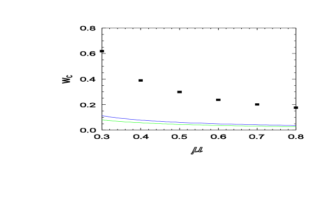
Figure 7: (Color online) Critical rate $w_{c}$ versus parameter $\mu$ for ${\cal D}=0.02$ and other parameters as in Fig. 6. Points: simulation; solid curves: diffusive MFT (upper) and simple MFT (lower). Error bars are smaller than the symbols.

IV.1 Critical behavior

Following preliminary studies which indicated that $w_{c}\simeq 0.297$, (for the parameter set mentioned above, with ${\cal D}=0.02$), we performed a more detailed study using $L=360$ and $t_{M}=5\,000$, with 72 000 realizations for each value of $w$ studied. A large number of realizations is necessary to obtain a clear result for $w_{c}$ and the critical exponents. Using a set of 10³ or 10⁴ realizations (a number that would be sufficient for studying the contact process, for example) the results are dominated by fluctuations. We believe that this is due to the multi-step nature of propagation, and in particular, to diffusion. For the relatively small diffusion rate used here, the initial stages of propagation depend on rare events, whereas for large values of ${\cal D}$, we expect that long simulations of large systems would be needed to observe the crossover from mean-field-like behavior to the asymptotic scaling regime.

The spreading exponents $\theta$, $\delta$ and $z_{sp}$ are estimated via analysis of the local slopes, $\theta(t)$, etc. For example, $\theta(t)$ is defined as the inclination of a least-square linear fit to the data for $n(t)$ (on logarithmic scales), on the interval $[t/a,\,at]$. (The choice $a$ represents a compromise between high resolution, for smaller $a$, and insensitivity to fluctuations, for larger values; we use $a$ in the range 2-3.) We estimate the exponents by plotting the local slopes versus $1/t$ and extrapolating to $1/t=0$. Since a supercritical process leads to local slopes that curve upward, and vice-versa, we seek the value of $w$ associated with the least curvature. The local slopes are plotted in Fig. 8. On this basis of these results we estimate the critical point as $w_{c}=0.2972(1)$, and find $\theta=0.573(5)$, $\delta=0.096(1)$ and $z_{sp}=1.768(2)$. (The estimate for $w_{c}$ is based on the data for $\theta(t)$.) The results for the exponents compare reasonably well with the literature values, $\theta=0.586$, $\delta=0.092$, and $z_{sp}=1.771$ for dynamic percolation in two dimensions Hav ; Munoz . The main source of uncertainty in the exponent estimates is the uncertainty in $w_{c}$ itself. The exponents obey the scaling relation of dynamic percolation, $\theta=z_{sp}-2\delta-1$, to within uncertainty.

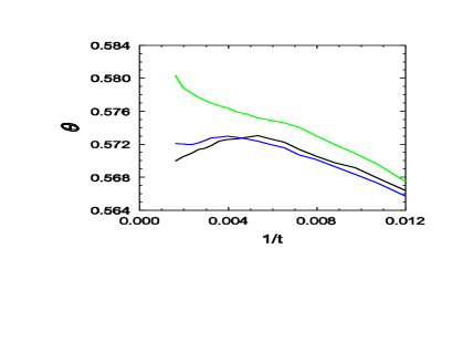
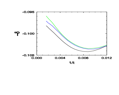
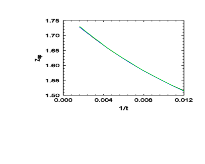
Figure 8: Simulation: local slopes $\theta(t)$, $\delta(t)$, and $z_{sp}(t)$ for (lower to upper, on left) $w=0.297$, 0.2972, and 0.2975. Parameters: ${\cal D}=0.02$, $\lambda=0.05$, $\mu=0.5$, $\nu=0.1$, and $w_{TR}=w_{DR}=w_{TS}=w_{DS}=0.2$.

To determine the fractal dimension of the critical cluster, we studied the radius of gyration $R_{g}$ of the final cluster as a function of its size, $n$, in a set of 500 realizations using $t_{M}=5000$. One expects that at the critical point, $R_{g}\propto n^{1/D_{f}}$, for $n\gg 1$ stauf . A least-squares linear fit to the data (see Fig. 9) yields $R_{g}\sim n^{0.525(6)}$, corresponding to a fractal dimension of $D_{F}=1.91(2)$. The value for two-dimensional percolation is 91/48 $\simeq$ 1.896 stauf .

Figure 9: Simulation: radius of gyration $R_{g}$ versus cluster size $n$ at the critical point for parameters as in Fig. 8, with $w=0.2972$.

IV.2 Subcritical regime

In the subcritical (nonspreading) regime, three quantities of interest are the mean lifetime $t_{p}$, the mean (final) cluster size $n$ and the mean radius of gyration $R_{g}$ of the final cluster. One expects that, in the neighborhood the critical point, these quantities scale as Hav ,

$${t_{p}\propto\Delta^{-\nu_{\parallel}}},\\ \quad n\propto\Delta^{-\zeta},\\ \quad R_{s}\propto\Delta^{-\nu_{\perp}}\\$$ (21)

where $\Delta=w_{c}-w$, and $\zeta=\gamma\nu_{\parallel}/\nu_{\perp}$, with $\gamma$ the percolation critical exponent governing the divergence of the mean cluster size.

We estimate the exponents $\nu_{\parallel}$, $\zeta$ and $\nu_{\perp}$ using simulations with system size $L=1000$, and 1000 realizations for each value of $w$ studied, for the parameter set defined above (see Fig. 10). The simulation results yield the estimates $\nu_{\parallel}=1.52(2)$, $\nu_{\perp}=1.29(3)$, and $\zeta=2.69(3)$. (We note, however, that the result for $\nu_{\perp}$ should not be taken very seriously, given the small values of $R_{g}$.) The reference values for dynamic percolation in two dimensions are $\nu_{\parallel}=1.506$, $\nu_{\perp}=4/3$, and $\zeta=2.698$ Hav .

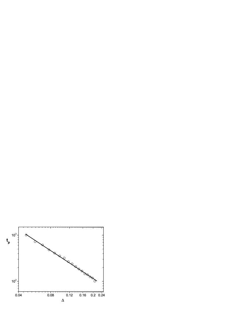
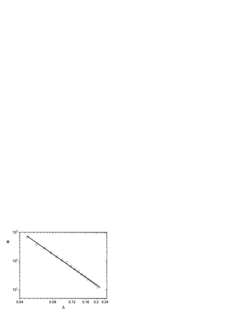
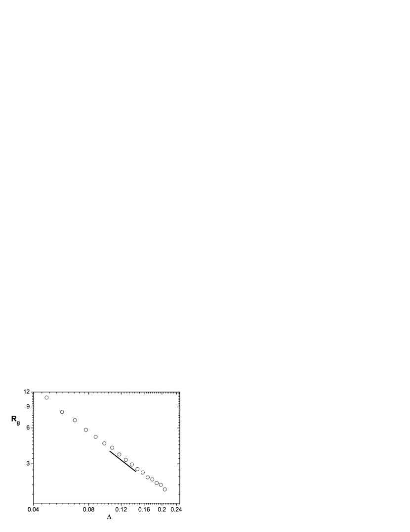
Figure 10: Simulation: survival time $t_{p}$, mean cluster size $n$, and mean radius of gyration $R_{g}$ versus $\Delta=w_{c}-w$, in the subcritical regime, for parameters as in Fig. 8. The slopes of the regression lines are 1.52 ($t_{p}$), 2.68 ($n$), and 1.29 ($R_{g}$).

IV.3 Clusters and spreading

Figure 11 shows examples of growing clusters at the critical point for two rather different values of the diffusion rate. The one corresponding to a smaller ${\cal D}$ value is more densely connected, while the other shows evidence of “colonies” growing at some distance from the main concentration, as well as a more diffuse boundary. The distribution of transformed and depleted cells around the perimeter is highly nonuniform in both cases. Further growth appears to be likely only in limited areas, as reflected in the nonuniform signal concentration. In the supercritical regime, cluster growth is more symmetric, but still somewhat irregular, as shown in Fig. 12, for parameters such that $w\simeq 1.08w_{c}$ and $1.33w_{c}$.

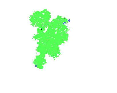
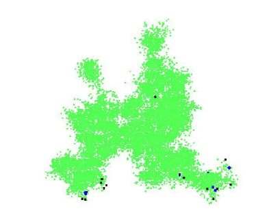
Figure 11: Growing critical clusters at time 2000, for parameters as in Fig. 6, with ${\cal D}=0.02$, $w=w_{c}=0.2972$ (left), and ${\cal D}=0.3$, $w=w_{c}=0.0812$ (right). Light color: removed cells; black dots: transformed cells; black diamond: position of original seed; $\times$: positions of relatively high signal concentration, $C>0.1$.

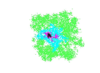
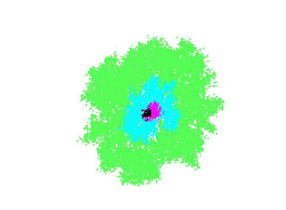
Figure 12: Growing clusters in the spreading regime. Contrasting colors show the set of removed cells at times 100, 200, 500, and 1000. Parameters as in Fig. 6, with ${\cal D}=0.1$. (For these parameters $w_{c}=0.1205(5)$.) Left panel: $w=0.13\simeq 1.08w_{c}$; right: $w=0.16\simeq 1.33w_{c}$.

We close this section with results on the propagation velocity $v_{s}$ in the spreading phase. Near the critical point (or the critical line in the $w$-${\cal D}$ plane) the velocity is expected to scale as $v_{s}\sim\epsilon^{\nu_{||}-\nu_{\perp}}$, where $\epsilon$ is the distance from criticality grass1 . This gives $v_{s}\sim\epsilon^{0.173}$ for dynamic percolation in two dimensions. In simulations, we determine the spreading velocity via the relation $\langle N_{R}(t)\rangle\simeq\pi(v_{s}t)^{2}$, i.e., the region of removed cells tends, on average, to a circle of radius $v_{s}t$ at long times. In these studies we perform $\sim 100$ realizations for each $w$ value, on lattices with $L=850$ - 1000, extending to a maximum time of $t_{M}=8000$ units. The results (Fig. 13) are consistent with a power law near the critical point. A fit to the data, using $w_{c}=0.1206$, yields $\nu_{||}-\nu_{\perp}=0.178(15)$; including the uncertainty in $w_{c}$ itself ($\pm 0.0001$), we obtain $\nu_{||}-\nu_{\perp}=0.18(4)$, which, while not very precise, is consistent with the value expected for dynamic percolation. The inset of Fig. 13 confirms the scaling $v_{s}\sim\sqrt{\cal D}$, as expected on the basis of dimensional analysis, away from the immediate vicinity of the critical point.

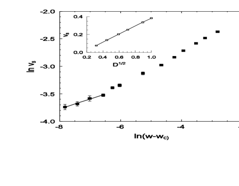
Figure 13: Simulation: spreading velocity $v_{s}=\langle N_{R}\rangle^{1/2}/(\sqrt{\pi}t)$ versus $w$ for ${\cal D}=0.1$. The slope of the regression line is 0.178. Inset: spreading velocity versus ${\cal D}^{1/2}$ for $w=0.15$. Other parameters as in Fig. 8. Lines are a guide for the eye.

V Discussion

We study an epidemic model consisting of elements (organisms in a community or cells in tissue) with fixed positions, in which disease or damage is transmitted by diffusing signals emitted by infected individuals. The model is formulated on a square lattice in which each site bears a cell, which can be in one of the states: susceptible, transformed, depleted, or removed. Signal diffusion and decay is treated deterministically, given the (random) source distribution in space and time. We study the model using mean-field theory (in both simple and diffusive versions) and Monte Carlo simulation. Simple MFT predicts the order of magnitude of the critical value $w_{c}$, if the diffusion rate is not extremely small, but is insensitive to the diffusion rate. Diffusive MFT yields a slight improvement over the simpler analysis; it captures, qualitatively, the fact that $w_{c}$ decreases with ${\cal D}$, and that $w_{c}$ diverges as ${\cal D}\to 0$.

The process is found to exhibit a continuous phase transition between spreading and nonspreading phases. Simulations of the spread of activity yield estimates for the critical exponents $\theta$, $\delta$, and $z_{sp}$ consistent with those of two-dimensional dynamic percolation. The fractal dimension of the cluster of affected individuals at the critical point is also consistent with that of dynamic percolation, as are the critical exponents associated with the subcritical regime, and the scaling of the spreading velocity in the supercritical regime. Although these results are obtained for a specific set of parameters, there is little reason to expect a change in scaling behavior for other values, as long as the diffusion rate is finite. Indeed, dynamic percolation universality for epidemic-like processes with a finite range of spreading was already asserted some time ago grass1 . We are unaware, however, of a previous verification of such behavior in the case of propagation via a diffusing, decaying signal.

The present study suggests several lines for future work. One is a more detailed study of the scaling of the spreading velocity. The ability of mean-field theory or reaction-diffusion equations to describe this aspect of the process is of interest, as such approaches are frequently used in applications. Another subject for future study concerns the nature of the spreading transition in disordered and fractal media. The possibility of a discontinuous transition for a nonlinear dependence of the transformation rate on signal concentration is also worth investigating. While mean-field theory does predict such a transition when the concentration-dependent rates are $\propto C^{2}$, experience with contact-process-like models suggests that the nature of the transition depends on the details of the dynamics grass82 ; evansCP2 . Finally, applications to specific processes, such as the radiation-induced bystander effect, are of great interest, if plausible estimates of the governing rates can be obtained.

Acknowledgments

We thank C. H. C. Moreira for helpful discussions. F. P. Faria is grateful for support provided by Fapemig, Minas Gerais, Brazil. R. D. acknowledges financial support from CNPq, Brazil.

References

- (1) D. Mollison, J. R. Stat. Soc. Ser. B. Methodol. 39, 283 (1977).
- (2) J. D. Murray, Mathematical Biology, vols. 1 and 2, (Springer, New York, 2003).
- (3) P. Grassberger, Math. Biosc. 63, 157 (1983).
- (4) J. Cardy and P. Grassberger, J. Phys. A 18, L267 (1985).
- (5) F. Linder, J. Tran-Gia, S. R Dahmen, and H. Hinrichsen, J. Phys. A: Math. Theor. 41 (2008).
- (6) D. R. de Souza and T. Tomé, Physica A 389, 1142 (2010).
- (7) M. S. Bartlett, Stochastic Population Models in Ecology and Epidemiology, (Metheun, London, 1960).
- (8) H. Nikjoo and I. K. Khvostunov, Int. J. Radiat. Biol. 79, 43 (2003).
- (9) C. Mothersill and C. B. Seymour, Int. J. Radiat. Biol. 71, 421, (1997).
- (10) C. Mothersill and C. B. Seymour, Radiat. Res. 149, 256 (1998).
- (11) N. T. J. Bailey, Biometrika 40, 177 (1953).
- (12) J. E. Satulovsky and T. Tomé, Phys. Rev. E 49, 5073 (1994).
- (13) J. E. Satulovsky and T. Tomé, J. Math. Biol. 35, 344 (1997).
- (14) T. Tomé and R. M. Ziff, Phys. Rev. E 82, 051921 (2010).
- (15) K. Kuulasmaa, J. Appl. Probab. 19, 745 (1982).
- (16) L. M. Sander, C. P. Warren, and I. M. Sokolov, Physica A 325, 1 (2003).
- (17) B. Gönci, V. Németh, E. Balogh, B. Szab , . D nes, Z. K rnyei, and T. Vicsek, PLoS ONE 5(12): e15571 (2010).
- (18) M. Henkel, H. Hinrichsen, and S. Lübeck, Non-Equilibrium Phase Transitions: Absorbing Phase Transitions, vol. 1, (Springer, New York, 2009).
- (19) T. E. Harris, Ann. Prob. 2, 969 (1974).
- (20) J. Marro, and R. Dickman, Nonequilibrium Phase Transitions in Lattice Models (Cambridge University Press, Cambridge, 1999).
- (21) W. O. Kermack and A. G. McKendrick, Proc. Royal Soc. London A 115, 700 (1927).
- (22) D. J. Daley and J. Gani, Epidemic Modelling, (Cambridge University Press, Cambridge, 1999).
- (23) F. Schlögl, Z. Phys. 253, 147 (1972).
- (24) P. Grassberger and A. de la Torre, Ann. Phys. (N. Y.) 122, 373 (1979).
- (25) D. Stauffer and A. Aharony, Introduction to Percolation Theory, 2nd Ed., (Taylor and Francis, London, 1992).
- (26) A. Bunde and S. Havlin, in Fractals and Disordered Systems, A. Bunde and S. Havlin, Eds. (Springer-Verlag, Heidelberg,1991).
- (27) M. A. Muñoz, R. Dickman, A. Vespignani and S. Zapperi, Phys. Rev. E 59, 6175-6179 (1999).
- (28) P. Grassberger, Z. Phys. B 47, 365 (1982).
- (29) D.-J. Liu, X. Guo, and J. W. Evans, Phys. Rev. Lett. 98, 050601 (2007).