Quench Dynamics of Topological Maximally-Entangled States

Abstract

We investigate the quench dynamics of the one-particle entanglement spectra (OPES) for systems with topologically nontrivial phases. By using dimerized chains as an example, it is demonstrated that the evolution of OPES for the quenched bi-partite systems is governed by an effective Hamiltonian which is characterized by a pseudo spin in a time-dependent pseudo magnetic field $\mathbf{S}(k,t)$. The existence and evolution of the topological maximally-entangled edge states are determined by the winding number of $\mathbf{S}(k,t)$ in the $k$-space. In particular, the maximally-entangled edge states survive only if nontrivial Berry phases are induced by the winding of $\mathbf{S}(k,t)$. In the infinite time limit the equilibrium OPES can be determined by an effective time-independent pseudo magnetic field $\mathbf{S}_{\mbox{eff}}(k)$. Furthermore, when maximally-entangled edge states are unstable, they are destroyed by quasiparticles within a characteristic timescale in proportional to the system size.

Topological phases that are not characterized by local order parameters have been subjects of key interests in condensed matter physics due to anomalous properties associated with these phases. Recent discovery of time-reversal invariant topological insulators Topo ; TopoExp has further triggered intense investigations on the characterization of topological phases. One of the important features for topological phases is the possibility of creating nonlocal properties associated with the topology, which is often realized as the entanglement between the system and its environment. In particular, the entanglement spectrum (ES) i.e. the eigenvalues of the reduced density matrix of the system, provides an idea tool to characterize the topological phase Haldane ; KitaevPollmann . In general, not only the ES can be used to distinguish different classification of topological phases but also it can detect the existence of edge modes at zero energy RyuHatsugai02 ; MJCY11 . The existence of edge states at zero energy reflects the non-trivial topology of the underlying quantum state. From the point of view for manipulating quantum information, these edge modes represent the maximally entangled states of the system and its environment. Therefore, they are the best candidate for qubits MJCY11 .

In order for the topological maximally-entangled state being a viable candidate for qubits, it is necessary to examine if they could survive under quantum information processing. Since typical quantum manipulations involve rapid change of the coupling to the environments, it is therefore important to examine the quench dynamics of maximally-entangled states. Recent investigations indicate that the thermalization of integrable systems due to quench depends strongly on the initial conditions ColdAtoms ; Rigol ; MingMiguelAnibal . These studies, however, are confined to the bulk properties. There are only few papers concerning quench dynamics of topological edge states Delgado . In the presence of topological edge states, the system can be maximally entangled with the environment and the thermalization of quench dynamics could be entirely different. It is thus important to examine the quench dynamics of topological maximally-entangled states. In this paper, by taking dimerized chain as an example, we investigate how edge states affect the thermalization and the quench dynamics of one-particle entanglement spectra (OPES) defined below. In particular, we show that the existence and evolution of topological maximally-entangled edge states are determined by the winding number of a pseudo magnetic field $\mathbf{S}(k,t)$. The maximally-entangled states survive only if nontrivial Berry phases are induced by the winding of $\mathbf{S}(k,t)$.

Consider the ground state $|\Psi_{AB}\rangle$ of a bipartite total system $AB$ that consists of the system $A$ and the environment $B$. The reduced density matrix of the system $A$ is $\rho_{A}=\operatorname{Tr}_{B}|\Psi_{AB}\rangle\langle\Psi_{AB}|$. The entanglement entropy (EE), defined as $S_{A}\equiv-\operatorname{Tr}\rho_{A}\log_{2}\rho_{A}$, has been widely used to measure the bipartite entanglement between the system $A$ and the environment $B$ Review . It is known that the scaling law of EE provides a way to distinguish different quantum phases AreaLaw . Furthermore, the property that EE diverges at the critical points provides a useful tool to examine the quantum criticality QCP . In addition to global properties associated with EE, it is useful to explore detailed microscopic quantum phenomena using OPES, defined as the set of $\lambda_{m}$’s with $\rho_{A}=\bigotimes_{m}\left[\begin{matrix}\lambda_{m}&0\\ 0&1-\lambda_{m}\end{matrix}\right]$. EE and OPES are related through the relation $S_{A}=\sum_{m}S_{m}$ where $S_{m}=-\lambda_{m}\log_{2}{\lambda_{m}}-(1-\lambda_{m})\log_{2}{(1-\lambda_{m})}$. The OPES has been used to investigate disorder lines MingPeschel , Berry phase RyuHatsugai06 ; MJCY11 and zero-energy edge states RyuHatsugai06 ; MJCY11 . It is clear that the eigenvalue $\lambda_{m}=1/2$ corresponds to the situation when the system $A$ and the environment $B$ are maximally entangled so that $S_{m}=1$. Since $\lambda_{m}=1/2$ is a mid-gap state that often results from the zero-energy edge state between $A$ and $B$, the maximally-entangle state is often topologically protected.

To investigate quench dynamics of the maximally-entangled state, we consider a one-dimensional (1D) dimerized chain characterized by the Hamiltonian:

$$H_{\delta}=-\sum_{i}(1+\delta(-1)^{i})(c_{i}^{\dagger}c_{i+1}+{\mbox{h.c.}}),$$ (1)

where $i$ is the site index and $\delta\in[-1,1]$. The ground state undergoes a phase transition from a topologically trivial phase ($\delta<0$) to a topologically nontrivial phase ($\delta>0$) as $\delta$ is varied across the phase boundary $\delta_{c}=0$. Let the region $i>0$ represents the system $A$ while $i\leq 0$ represents the environment $B$, the topological edge mode appears if the bond $[i,i+1]=[0,1]$ is strong, i.e., $-(1+\delta)<-(1-\delta)$. Otherwise the edge mode does not exist wu . In this paper we study the quench dynamics of the topological maximally-entangled states for a dimerized chain by suddenly quenching the parameter $\delta$.

The occurrence of maximally-entangled edge states has its topological origin. By defining a spinor $\mathbf{c}_{x_{i}}=(c_{x_{i1}},c_{x_{i2}})^{\operatorname{T}}$ where $x_{i1}=2i-1$ and $x_{i2}=2i$ and performing a Fourier transformation, the Hamiltonian (1) can be casted into the form

$$H_{\delta}=-\sum_{k\in BZ}\mathbf{c}_{k}^{\dagger}[\mathbf{R}_{\delta}(k)\cdot\boldsymbol{\sigma}]\mathbf{c}_{k},$$ (2)

where $\boldsymbol{\sigma}=(\sigma_{x},\sigma_{y},\sigma_{z})$ are Pauli matrices and

$$\mathbf{R}_{\delta}(k)=\left((1-\delta)+(1+\delta)\cos{k},(1+\delta)\sin{k},0\right)$$ (3)

is a pseudo magnetic field with the magnitude $R_{\delta}(k)=2(\cos^{2}{k/2}+\delta^{2}\sin^{2}{k/2})^{1/2}$. The system fulfills chiral symmetry because $\mathbf{R}_{\delta}(k)$ lies on a plane. For $\delta\in(0,1]$ the loop $\ell$ of $\mathbf{R}_{\delta}(k)$ encloses the origin $\cal{O}$ as $k$ runs through the Brillouin zone. Consequently, the Berry phase (or Zak’s phase) $\chi$, defined as a line integral of the curvature of the filled band, is $\pi$. Due to the fact that $\ell$ can be continuously deformed into a unit circle without crossing the origin, topological argument ensures that the original Hamiltonian corresponding to $\ell$ contains at least one pair of one zero-energy edge states as a consequence of chiral symmetry RyuHatsugai02 . On the other hand, if $\delta\in[-1,0)$, one obtains trivial Berry phases and no topological edge state occurs (see the upper panels of Fig 1).

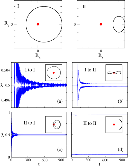
Figure 1: (color online) Upper two panels: Representative loops $\ell$ of $\mathbf{R}_{\delta}(k)$ for phase I and II with $\delta=0.5$ and $\delta=-0.5$ respectively. In phase I ($\delta\in(0,1]$) the Berry phase is $\pi$ due to circling of $\mathbf{R}_{\delta}(k)$ around the origin, while in phase II ($\delta\in[-1,0)$) the Berry phase is trivial. Lower four panels: evolutions of two $\lambda_{m}(t)$ that are closest to $1/2$ for different quench processes: (a) phase I ($\delta=0.5$) to I ($\delta=0.2$) (b) phase I ($\delta=0.5$) to II ($\delta=-0.5$) (c) phase II ($\delta=-0.5$) to I ($\delta=0.5$) (d) phase II ($\delta=-0.5$) to II ($\delta=-0.2$). Insets: loop $\ell$ of $\mathbf{S_{\mbox{eff}}}$

.

We consider a total system of infinite size, and partition it into the system $A$ with $x_{i}=1,\cdots,L/2$ and its environment $B$ (the remaining part). The reduced density matrix of the system $\rho_{A}$ for the ground state can be determined by eigenvalues $\lambda_{m}$ of the block Green’s function matrix (GFM) GFM $G^{\delta}_{\alpha\beta}(x_{i},x_{j})=\operatorname{Tr}[\rho c_{x_{i\alpha}}^{\dagger}c_{x_{j\beta}}]$, where $x_{i\alpha},x_{j\beta}$ belong to the system $A$, $\alpha,\beta=1,2$, and $\rho$ is the ground state density matrix of the total system. Hence the GFM can be considered as an effective Hamiltonian that determines the OPES. In the Fourier $k$-space, $G^{\delta}_{\alpha\beta}(k)$ is given by

$$G^{\delta}_{\alpha\beta}(k)=\frac{1}{2}\left[1+\hat{\mathbf{R}}_{\delta}(k)\cdot\boldsymbol{\sigma}\right]_{\alpha\beta},$$ (4)

where $\hat{\mathbf{R}}_{\delta}(k)=\mathbf{R}_{\delta}(k)/R_{\delta}(k)$. It takes almost the same form as the Hamiltonian (2) except for a constant and a positive normalization factor $R_{\delta}$, which leads to the conclusion that they share the same topology. If $\mathbf{R}_{\delta}(k)$ encloses the origin in the parameter space with Berry phase equal to $\pi$, a pair of zero energy states appear for the Hamiltonian (2), while for the GFM, we obtain a pair of maximally-entangled states with $\lambda_{m}=1/2$. Notice that the maximally-entangled states are also edge states, which can be seen in Fig 3.

Consider now a sudden quench at $t=0$ by changing the parameter of the dimerized chain in Eq. (1) from $\delta$ at $t<0$ to $\delta^{\prime}$ at $t>0$. Denote the phase whose $\delta\in(0.1]$ with maximally-entangled states by phase I, and the phase whose $\delta\in[-1,0)$ by phase II. We perform four possible quench processes, including I to I, I to II, II to I, and II to II. The OPES $\lambda_{m}(t)$ at time $t$ can be obtained by diagonalizing a time-dependent GFM which is defined as $G_{\alpha\beta}(x_{i},x_{j},t)=\operatorname{Tr}(\rho e^{iH_{\delta^{\prime}}t}c_{x_{i\alpha}}^{\dagger}c_{x_{j\beta}}e^{-iH_{\delta^{\prime}}t})$ where $x_{i},x_{j}\in A$ CalabreseCardy . In Fig 1 (a)-(d), we show the time evolution of OPES for states whose eigenvalues are closest to $1/2$. In cases of I to I and I to II, the maximally-entangled states persist for a while and then split into two different evolutions. Only for the case of I to I, however, the two splitting eigenstates evolve back to two maximally-entangled states at infinite time. In contrast, for the case of I to II, two splitting eigenstates closest to $1/2$ remain splitting forever. On the other hand, if one starts with initial states without maximally-entangled states such as the cases of II to I and II to II, maximally-entangled states can not be created at later time.

It is instructive to define a time-dependent pseudo magnetic field $\mathbf{S}(k,t)$ from the time-dependent GFM $G(k,t)$ in the Fourier space through the relation

$$G_{\alpha\beta}(k,t)=1/2\left[1+\mathbf{S}(k,t)\cdot\boldsymbol{\sigma}\right]_{\alpha\beta}.$$ (5)

$\mathbf{S}(k,t)$ can be further written as a summation of three different contributions

$$\mathbf{S}_{1}(k,t) = \cos(2R_{\delta^{\prime}}t)\hat{\mathbf{R}}_{\delta}(k),$$ (6)

$$\mathbf{S}_{2}(k,t) = \sin(2R_{\delta^{\prime}}t)\hat{\mathbf{R}}_{\delta}(k)\times\hat{\mathbf{R}}_{\delta^{\prime}}(k),$$ (7)

$$\mathbf{S}_{3}(k,t) = (1-\cos(2R_{\delta^{\prime}}t))\hat{\mathbf{R}}_{\delta}(k)\cdot\hat{\mathbf{R}}_{\delta^{\prime}}(k)\hat{\mathbf{R}}_{\delta^{\prime}}(k).$$ (8)

The thermalization of EE observed in Fig 1 can be understood by considering the infinite-time limit of the time-dependent pseudo magnetic field (6), (7), and (8). Since the sinusoidal parts dephase out, the long-time behavior of the time-dependent GFM, $G_{\alpha\beta}(k,t=\infty)$, is solely determined by the effective pseudo magnetic field

$$\mathbf{S}_{\mbox{eff}}(k)\equiv\left(\hat{\mathbf{R}}_{\delta}(k)\cdot\hat{\mathbf{R}}_{\delta^{\prime}}(k)\right)\hat{\mathbf{R}}_{\delta^{\prime}}(k).$$ (9)

The existence of maximally-entangled states at infinite time is thus determined by the topology of $\mathbf{S}_{\mbox{eff}}$. If $\mathbf{S}_{\mbox{eff}}$ encircles origin, the Berry phase is $\pi$, maximally-entangled states appear at $t=\infty$; otherwise there is no maximally-entangled state at later time. It is clear that both the final $\mathbf{R}_{\delta^{\prime}}$ and the initial $\mathbf{R}_{\delta}$ determine $\mathbf{S}_{\mbox{eff}}$. It implies that the long time behavior carries the memory of the initial state, which is due to nonergodicity of integrable systems MingMiguelAnibal . The existence of maximally-entangled states (edge states) at infinite time requires that both the initial and final Hamiltonians possess nontrivial Berry phase. In the inset of Fig 1(a)-(d), $\mathbf{S}_{\mbox{eff}}$ are plotted for different quench processes with different initial and final Hamiltonians. It is clear that only for the quench from I to I, $\mathbf{S}_{\mbox{eff}}$ encircles origin, while in the other quenches $\mathbf{S}_{\mbox{eff}}$ either not encircles the origin (II to II) or passes through the origin (I to II or II to I).

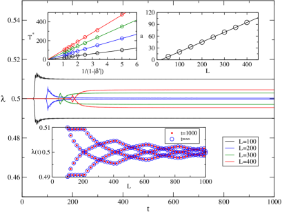
Figure 2: (color online) Evolutions of two $\lambda_{m}(t)$ that are closest to $1/2$ for different $L$ under the quench of I ($\delta=0.5$) to II ($\delta=-0.5$). Lower inset: $\lambda_{m}(t)$ obtained from exact diagonalization of $G_{\alpha,\beta}(x_{i},x_{j},t=1000)$ (blue circle) and $\mathbf{S_{\mbox{eff}}}$ (red dots). Upper left panel: fitting of $T^{\star}$, the persistence time of the maximum entangled states, using $T^{\star}(L)=a(L)/(1-|\delta^{\prime}|)$ where $T^{\star}$ is the persistence time of the maximum entangled states. Upper right panel: fitting of $a(L)$ versus $L$. We find that $a\approx 0.232L$.

The reason is that if the initial state is in the same phase as the final Hamiltonian (I to I or II to II), $\hat{\mathbf{R}}_{\delta}(k)\cdot\hat{\mathbf{R}}_{\delta^{\prime}}(k)$ is always positive, therefore the topology of $\mathbf{S}_{\mbox{eff}}$ is the same as $\hat{\mathbf{R}}_{\delta^{\prime}}(k)$. On the other hand, if the system is quenched into a phase that is distinctly from the initial state, $\hat{\mathbf{R}}_{\delta}(k=0)\cdot\hat{\mathbf{R}}_{\delta^{\prime}}(k=0)$ is positive while $\hat{\mathbf{R}}_{\delta}(k=\pi)\cdot\hat{\mathbf{R}}_{\delta^{\prime}}(k=\pi)$ is negative, then there must exist one point $k_{0}$ that $\mathbf{S}_{\mbox{eff}}(k_{0})\propto\hat{\mathbf{R}}_{\delta}(k_{0})\cdot\hat{\mathbf{R}}_{\delta^{\prime}}(k_{0})=0$. Hence, $k_{0}$ destroys the topology of the infinite-time Green’s function matrix. There exist no maximally-entangled states whenever the system is quenched across the topological phase boundary. This explains why only the quench from phase I to phase I creates maximally-entangled states at infinite time.

For all cases shown in Fig 1, the OPES $\lambda_{m}(t)$ of the dimerized chain fluctuate before it reaches the equilibrium. The intermediate regions can be explained by the appearance of $\mathbf{S}_{2}$ in the time-dependent GFM. Since $\mathbf{S}_{2}$ is proportional to $\hat{\mathbf{R}}_{\delta}(k)\times\hat{\mathbf{R}}_{\delta^{\prime}}(k)$ and is perpendicular to $\mathbf{S}_{1}$ and $\mathbf{S}_{3}$, the system is agitated by quasiparticles induced by $\mathbf{S}_{2}$ and $\mathbf{S}_{3}$ until the time-dependent sinusoidal functions dephase out and then the system reaches its equilibrate state with the effective $\mathbf{S}_{\mbox{eff}}$ (9). Clearly, the thermalization depends on sizes of the system $A$. To check the size dependence, Fig 2 shows several quench processes from phase I to phase II with different system length. In the lower panel, we compare eigenvalues at $t=1000$ (red dots) evolved from the maximally-entangled state with eigenvalues obtained by diagonalization of $G_{\alpha\delta}(\mathbf{k},\infty)$ (blue circles). The dependence on the system size $L$ shows excellent agreement, indicating the validity of $\mathbf{S}_{\mbox{eff}}$.

We also find that if the initially the system is in phase I, the maximally-entangled states can persist for a long time $T^{\star}$ before they are destroyed. This feature is striking because the maximally-entangled states are not destroyed in the beginning. Furthermore $T^{\star}$ is independent of the initial conditions but depends on the final Hamiltonian and the system length $L$. This is because the maximally-entangled states reside on the edge MJCY11 and they will disappear only when the quasiparticles created from the bulk reach the edges. Therefore, we expect $T^{\star}\approx L/(2v_{\mbox{max}})$, where $v_{\mbox{max}}$ is the maximum velocity of the quasiparticles. For the energy dispersion on obtains $v_{\mbox{max}}=2(1-|\delta^{\prime}|)$ hence

$$T^{\star}\approx\frac{L}{4(1-|\delta^{\prime}|)}.$$ (10)

In the upper left inset of Fig 2, we show the fitting of $T^{\star}(L)$ to the function $a(L)/(1-|\delta^{\prime}|)$ using various system size $L$. We then fit $a(L)=b\times L$ as shown in the upper right inset of Fig 2 to find $b\approx 0.232$. Combining these two fitting we find that $T^{\star}\approx 0.232L/(1-|\delta^{\prime}|)$ which is very closed to our approximation Eq. (10). Our results imply that edge modes remains to the infinite time if $L$ is infinite. Therefore, the edge modes serve as good qubits since they have the maximal entanglements and cannot be destroyed easily if the system is large enough.

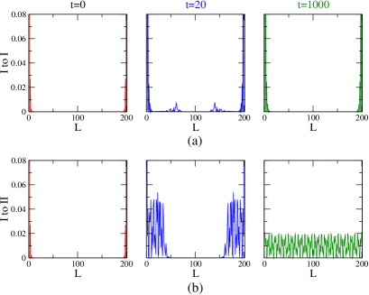
Figure 3: The probability sum of the two eigenstates whose eigenvalues are closest to $1/2$. (a) Quench process I to I. The edge modes persist from the beginning to the end. (b) Quench process I to II. The edge modes disappear and evolve to the bulk state.

The disappearance and recreation for different quench process starting from the phase I can be further explored by examining the probability sum of the two eigenstates with eigenvalues being closest to $1/2$. Fig 3(a) shows the case of I to I. It is seen that only small amounts of quasiparticles are excited. As a result, the edge modes remain from the beginning to the end. On the other hand, for the quench process I to II as shown in Fig 3(b), quasiparticles strongly modify two edge modes until they disappear and the whole system is bulk-like without any edge mode.

In summary, using dimerized chains as an example, the quench dynamics of the maximally-entangled states is investigated by diagonalizing the time-dependent Green’s function matrix. We find that the existence of the maximally-entangled states after sudden quench is determined by an effective pseudo magnetic field ($\mathbf{S}_{\mbox{eff}}$), which depends on both the initial and final Hamiltonians. The topological properties at infinite time are thus determined by the initial states and the Hamiltonian after the quench. When the maximally-entangled states are unstable, they are destroyed by quasiparticles that move from the bulk to the edges with a characteristic timescale proportional to the system size.

We thank Dr. Sungkit Yip for useful discussions. This work was supported by the National Science Council of Taiwan.

References

- (1) C. L. Kane and E. J. Mele, Phys. Rev. Lett. 95, 146802 (2005); B. A. Bernevig, T. L. Hughes, and S.-C. Zhang, Science 314, 1757 (2006); L. Fu, C. L. Kane, and E. J. Mele, Phys. Rev. Lett. 98, 106803 (2007); J. E. Moore and L. Balents, Phys. Rev. B 75, 121306 (2007).
- (2) M. Konig, S.Wiedmann, C. Brune, A. Roth, H. Buhmann, L.W. Molenkamp, X.-L. Qi, and S.-C. Zhang, Science 318, 766 (2007); D. Hsieh, D. Qian, L. Wray, Y. Xia, Y. S. Hor, R. J. Cava, and M. Z. Hasan, Nature (London) 452, 970 (2008), 0902.1356.
- (3) Li H. and Haldane F. D. M., Phys. Rev. Lett., 101 (2008) 010504.
- (4) L. Fidkowski and A. Kitaev, Phys. Rev. B 81, 134509 (2010); A. M. Turner, Frank Pollmann, and Erez Berg, Phys. Rev. B 83, 075102 (2011)
- (5) S. Ryu and Y. Hatsugai, Phys. Rev. Lett. 89, 077002(2002).
- (6) M.-C. Chung, Y.-H. Jhu, P. Chen, and S.K. Yip, Eur. Phys. Lett. 95 27003 (2011).
- (7) S. Ryu and Y. Hatsugai, Phys. Rev. B 73, 245115 (2006).
- (8) T. Kinoshita, T. Wenger, and D. S. Weiss, Nature (London) 440, 900 (2006); S. Hofferberth et al. Nature (London) 449, 324 (2007); M. Greiner et al., Nature (London) 419, 51 (2002); S. Trotsky et al. arxiv: 1101.2658 (2011); J Simon, W S Bakr, R Ma, M E Tai, P M Preiss, M Greiner, 472, 307, Nature (2011)
- (9) M. Rigol, V. Dunjko, V. Yurovsky, and M. Olshanii, Phys. Rev. Lett. 98, 050405 (2007); M. Rigol, A. Muramatsu and M. Olanshii, Phys. Rev. A 74, 053616 (2006).
- (10) M.A. Cazalilla, A. Iucci and M.-C. Chung, Phys. Rev. E 85, 011133 (2012); M.-C, Chung, A. Iucci, and M. A. Cazalilla, arXiv: 1203.0121.
- (11) A. Bermudez, D. Patane, L. Amico, M. A. Martin-Delgado, Phys. Rev. Lett. 102, 135702 (2009); A. Bermudez, L. Amico, M. A. Martin-Delgado, New J. Phys. 12:055014, (2010)
- (12) For a review, see I. Peschel and V. Eisler, J. Phys. A : Math. Theor., 42, 504003 (2009).
- (13) For a review, see J. Eisert, M. Cramer and M.B. Plenio, Rev. Mod. Phys.82, 277 (2010).
- (14) A. Osterloh, L. Amica, G. Falci and R. Fazio, Nature 416, 608(2002). (2002);T. J. Osborne and M. A. Nielson, Phys. Rev. A 66, 032110 (2002).
- (15) S. T. Wu and C. Y. Mou, Phys. Rev. 66, 012512 (2002); Phys. Rev. B. 67, 024503 (2003); B.-L. Huang, S.-T. Wu, and C.-Y. Mou, Phys. Rev. B, 70, 205408 (2004).
- (16) M. C. Chung and I. Peschel, Phys. Rev. B 64, 064412 (2001).
- (17) I. Peschel, J. Phys. A 36, L205 (2003); S. A. Cheong and C. L. Henley, Phys. Rev. B 69, 075111 (2004); T. Barthel et. al Phe. Rev. A 74, 022329 (2006).
- (18) P. Calabrese and J. Cardy, J. Stat. Mech. 0504:P04010 (2005)