Visibility of ultracold Bose system in triangular optical lattices

Abstract

In this paper, by treating the hopping parameter in Bose-Hubbard model as a perturbation, with the help of the re-summed Green’s function method and cumulants expansion, the momentum distribution function of the ultra-cold Bose system in triangular optical lattice is calculated analytically. By utilizing it, the time-of-flight absorption picture is plotted and the corresponding visibility is determined. The comparison between our analytical results and the experimental data from Ref.[sengstock, ] exhibits a qualitative agreement.

I Introduction

During the past decade, the properties of ultra-cold atomic gases in optical lattices Markus-Greiner have received a great deal of attention on account of their novelty and various potential applications Immanuel-Bloch . In the case of bosons, the delicate balance between the atom-atom on-site repulsion and the hopping parameter leads to a Mott insulator-Superfluid (MI-SF) quantum phase transition which has been confirmed experimentally Markus-Greiner . Due to the precisely controllable parameters, the optical-lattice-ultra-cold-atom systems play roles of test ground for quantum many-body systems in condensed matter physics, this is the so-called quantum simulation lewenstein-1 .

Beside the simple cubic optical lattices, in which almost all experiments with ultra-cold atoms to date have been performed due to the ease of the ease of the implementation, the triangular and hexagonal optical lattices have also been recognized recently sengstock . In fact, due to the complexity of the lattice structure in these systems, novel and rich new phases will be exhibited, for instance, the effects of geometrical frustration have been achieved in triangular optical lattice cold atomic system experimentally sengstock-science ; Eckardt . Hence, it is worth to investigate these systems, especially their quantum phase transitions, in a systematic way.

In our previous work jiang-pra , we have calculated the phase boundaries of MI-SF quantum phase transitions of ultra-cold bosons in triangular, hexagonal, as well as Kagomé optical lattices analytically via the method of the field-theoretical effective potential axel , the relative deviation of our analytical results from the numerical results numerical-results is less than 10%. However, these results cannot be compared with the experimental observation, since the phase boundaries of the ultra-cold system are not able to be detected directly in experiments. Instead, time-of-flight measurement Immanuel-Bloch , which reveals the momentum distribution of the system, is the standard experimental technique for investigating cold atom systems in optical lattices Markus-Greiner1 ; Michael .

In this paper, by treating the hopping parameter as a perturbation, with the help of Green’s function calculation Metzner ; ohliger , we are going to calculate the time-of-flight absorbtion pictures and the associated visibility as well analytically for ultra-cold scalar bosons in triangular optical lattice. Our results exhibit a qualitative agreement with the experimental data.

II The model

As is well known, a system of scalar bosons trapped in a homogeneous optical lattice is portrayed by the many-body Hamiltonian which takes the form as

$$H=\int d{\bf r}\psi^{\dagger}(\textbf{r})\left(-\frac{\hbar^{2}}{2m}{\nabla^{2}}+V(\textbf{r})\right)\psi(\textbf{r})+\frac{g}{2}\int d\textbf{r}\psi^{\dagger}(\textbf{r})\psi^{\dagger}(\textbf{r})\psi(\textbf{r})\psi(\textbf{r}),$$ (1)

with $\psi(\textbf{r})$ ($\psi^{\dagger}(\textbf{r})$) being annihilation (creation) bosonic field operators and $V(\textbf{r})$ being the optical lattice trapping potential. The parameter $g$ is the interaction strength between two atomic particles.

In fact, due to the modulation of the optical lattice potential wells, in the extremely low temperature limit, a single band approximation is adequate, the bosonic field operators $\psi^{\dagger}(\textbf{r})$ and $\psi(\textbf{r})$ can be expanded in the basis of orthonormal Wannier functions $w(\textbf{r}-\textbf{r}_{j})$ of the lowest band jaksch-1 ; blakie as

$$\psi(\textbf{r}) = \sum_{j}\emph{w}\,(\textbf{r}-\textbf{r}_{j})\hat{a}_{j},$$

$$\psi^{\dagger}(\textbf{r}) = \sum_{i}\emph{w}^{\ast}\,(\textbf{r}-\textbf{r}_{i})\hat{a}_{i}^{\dagger},$$ (2)

where $\hat{a}_{i}^{\dagger}$ ($\hat{a}_{i}$) is the creation (annihilation) operator of scalar boson on site of $i$.

By utilizing the above expressions, the Hamiltonian in Eq.(1) is reduced in the tight-binding limit to the Bose-Hubbard Hamiltonian

$$\hat{H}_{\rm BH}=\hat{H}_{1}+\hat{H}_{0}$$ (3)

with the diagonal part $\hat{H}_{0}$ and the hopping part $\hat{H}_{1}$ being

$$\hat{H}_{0}=\sum_{i}\frac{U}{2}\hat{n}_{i}(\hat{n}_{i}-1)-\mu\hat{n}_{i},\,\,\,\hat{H}_{1}=-J\sum_{\langle i,j\rangle}\hat{a}_{i}^{\dagger}\hat{a}_{j},$$ (4)

respectively, where $\hat{n}_{i}=\hat{a}_{i}^{\dagger}\hat{a}_{i}$ is the particle number operator on site $i$. $J$ is the hopping amplitude for the bosons between the nearest neighbor sites $i$ and $j$ while $U$ denotes the on-site repulsion and $\mu$ is the chemical potential. As we can see from Eq.(1) to Eq.(4), $J$ and $U$ can be calculated explicitly by jaksch-1

$$J=-\int d{\bf r}w^{*}({\bf r}-{\bf r}_{i})\left(-\frac{\hbar^{2}\nabla^{2}}{2m}+V({\bf r})\right)w({\bf r}-{\bf r}_{j})$$ (5)

and

$$U=g\int d{\bf r}|w({\bf r})|^{4},$$ (6)

respectively, with ${\bf r}_{i}$ and ${\bf r}_{j}$ being nearest neighboring sites.

In experiment, the triangular optical lattice is created by three laser beams intersecting in the $x$-$y$ plane with angle of $2\pi/3$ between each other sengstock , the lattice constant of the obtained triangular lattice is $a=2\lambda/3$, where $\lambda$ is the wavelength of the lattice laser beams. The corresponding lattice trapping potential reads

$$V({\bf r})=V_{0}\left\{\frac{3}{4}-\frac{1}{2}\left[\cos\left(\frac{4\pi}{\sqrt{3}a}y\right)+\cos\left(\frac{2\pi}{\sqrt{3}a}y-\frac{2\pi}{a}x\right)+\cos\left(\frac{2\pi}{\sqrt{3}a}y+\frac{2\pi}{a}x\right)\right]\right\}.$$ (7)

Associated to this optical lattice trapping potential, in harmonic approximation, the corresponding Wannier function takes form of

$$w({\bf r}-{\bf r}_{i})=\left(\frac{32\widetilde{V}_{0}}{9}\right)^{\frac{1}{4}}\left(\frac{\pi}{a^{2}}\right)^{\frac{1}{2}}\exp\left[-\left(\frac{8\widetilde{V}_{0}}{9}\right)^{\frac{1}{2}}\frac{\pi^{2}}{a^{2}}\left((x-x_{i})^{2}+(y-y_{i})^{2}\right)\right]$$ (8)

with $\widetilde{V}_{0}$ being dimensionless optical lattice depth in unit of recoil energy $E_{R}=(\hbar^{2}k^{2})/2m$, where $k=2\pi/\lambda$.

III The momentum distribution function

Actually, the quantity that is measured in experiments is the distribution function in the momentum space prokofev-1

$$n(\mathbf{k})=\int d\mathbf{r}\,d\mathbf{r}^{\prime}e^{i\mathbf{k}\cdot(\bf r-\bf r^{\prime})}\langle\psi^{\dagger}(\bf{r})\psi(\bf{r^{\prime}})\rangle.$$ (9)

By making use of Eq.(2), with the help of the Fourier transformation of the operators

$$\hat{a}^{\dagger}_{i}=\frac{1}{\sqrt{N_{S}}}\sum_{\mathbf{k}_{1}}\hat{a}^{\dagger}_{\mathbf{k}_{1}}e^{-i\mathbf{k}_{1}\cdot\mathbf{r}_{i}},\,\,\,\hat{a}_{j}=\frac{1}{\sqrt{N_{S}}}\sum_{\mathbf{k}_{2}}\hat{a}_{\mathbf{k}_{2}}e^{i\mathbf{k}_{2}\cdot\mathbf{r}_{j}},$$ (10)

where $N_{S}$ is the total of the lattice number, the momentum distribution function is reduced to

$$n(\mathbf{k})=N_{S}\mid\emph{w}(\mathbf{k})\mid^{2}\langle\hat{a}^{\dagger}_{\mathbf{k}}\hat{a}_{\mathbf{k}}\rangle.$$ (11)

As is known, the one particle Green’s function in the momentum space reads

$$G(\tau\mid 0,\mathbf{k})=\,\langle\hat{T}_{\tau}[\hat{a}^{\dagger}(\tau)_{\mathbf{k}}\hat{a}(0)_{\mathbf{k}}]\rangle,$$ (12)

where $\tau$ is imaginary time and $\hat{T}_{\tau}$ is the imaginary time ordering operator. It is the Fourier transformation of the one particle Green’s function $G(\tau^{\prime},j^{\prime}\mid\tau,j)=\,\langle\hat{T}_{\tau}[\hat{a}^{\dagger}_{j^{\prime}}(\tau^{\prime})\hat{a}_{j}(\tau)]\rangle$. Apparently, $\langle\hat{a}^{\dagger}_{\mathbf{k}}\hat{a}_{\mathbf{k}}\rangle=\lim_{\tau\downarrow 0}G_{1}(\tau\mid 0,\mathbf{k})$, we then translate the problem of calculating the density distribution to a problem of calculating corresponding Green’s function.

However, due to the non-commutativity of the two parts of the full Hamiltonian (3), the exact information of the corresponding eigenstates can hardly be obtained. Nevertheless, the Green’s functions can be calculated perturbatively via the Dirac representation. To tackle the issue of time-of-flight absorbtion picture which is closely related to the MI-SF phase transition, we treat the hopping term in the Hamiltonian (3) as the perturbation part, for the opposite limit will not lead to a MI-SF phase transition at all stoof .

In Dirac picture, the time evolution of operators is only determined by the unperturbed part of the Hamiltonian (set $\hbar=1$) M. Peskin $\hat{O}(\tau)=e^{\tau\hat{H}_{0}}\hat{O}e^{-\tau\hat{H}_{0}}$, and the corresponding evolution operator takes the form of

$$\hat{u}(\beta,0)=\hat{T}_{\tau}\left[e^{\int^{\beta}_{0}d\tau\sum_{\langle i,j\rangle}J\hat{a}^{\dagger}_{i}(\tau)\hat{a}_{j}(\tau)}\right].$$ (13)

Without any difficulty, it can be proved that the one particle Green’s function reads

$$G(\tau^{\prime},j^{\prime}\mid\tau,j) = \,\frac{\text{Tr}\{{{e^{-\beta\hat{H}_{0}}}\hat{T}_{\tau}[\hat{a}^{\dagger}_{j^{\prime}}(\tau^{\prime})\hat{a}_{j}(\tau)\hat{u}(\beta,0)]}\}}{\{\text{Tr}{e^{-\beta\hat{H}_{0}}}\hat{u}(\beta,0)\}}.$$ (14)

To calculate $G(\tau^{\prime},j^{\prime}\mid\tau,j)$, the evolution operator $\hat{u}(\beta,0)$ has to be expanded perturbatively, i.e., the expansion express of $G(\tau^{\prime},j^{\prime}\mid\tau,j)$ consists of terms, for instance, as

$$\frac{1}{n!}\sum_{i_{1},j_{1},\cdots,i_{n},j_{n}}J_{i_{1},j_{1}}\cdots J_{i_{n},j_{n}}\int^{\beta}_{0}d\tau_{1}\cdots\int^{\beta}_{0}d\tau_{n}\langle\hat{T}_{\tau}[\hat{a}^{\dagger}_{j^{\prime}}(\tau^{\prime})\hat{a}_{j}(\tau)\hat{a}^{\dagger}_{i_{1}}(\tau_{1})\hat{a}_{j_{1}}(\tau_{1})\cdots\hat{a}^{\dagger}_{i_{n}}(\tau_{n})\hat{a}_{j_{n}}(\tau_{n})]\rangle_{0},$$ (15)

with $\langle\hat{O}\rangle_{0}$ being average quantity with respect to the unperturbed part $H_{0}$ of the Hamiltonian. Here, the $J_{ij}$ reads

$$J_{ij}=\begin{cases}J,\;\;\;&\text{if {\it i, j} are nearest neighbors of each other,}\\ 0,\;\;\;&\text{otherwise.}\end{cases}$$ (16)

Thus, the following quantities need to be calculated first

$$G^{(0)}_{n}(\tau^{\prime}_{1},i^{\prime}_{1};\cdots\tau^{\prime}_{n},i^{\prime}_{n}\mid\tau_{1},i_{1};\cdots\tau_{n},i_{n})=\langle\hat{T}_{\tau}[\hat{a}^{\dagger}_{i^{\prime}_{1}}(\tau^{\prime}_{1})\hat{a}_{i_{1}}(\tau_{1})\cdots\hat{a}^{\dagger}_{i^{\prime}_{n}}(\tau^{\prime}_{n})\hat{a}_{i_{n}}(\tau_{n})]\rangle_{0},$$ (17)

these are the $n$-particle Green’s function with respect to $H_{0}$. Unfortunately, the Wick’s theorem cannot be applied to calculate the above quantity, since the eigenstates of the non-perturbed part of the Hamiltonian (3) is local, and each annihilation operator in the expression should be paired with a creation operator on the same site, otherwise the result would be zero. Therefore, we should turn to the theory of linked-cluster expansion Metzner ; ohliger , i.e. to expand the $n$-particle Green’s function in terms of the cumulants $C^{(0)}_{m}(\tau^{\prime}_{1},\cdots,\tau^{\prime}_{m}\mid\tau_{1},\cdots\tau_{m})=\langle\hat{T}_{\tau}[\hat{a}^{\dagger}(\tau^{\prime}_{1})\hat{a}(\tau_{1})\cdots\hat{a}^{\dagger}(\tau^{\prime}_{m})\hat{a}(\tau_{m})]\rangle_{0}$ in which the particle operators are all on the same site.

By defining the generation function as

$$C^{(0)}_{0}[j,j^{\ast}]=\ln\langle\hat{T}_{\tau}e^{(\int^{\beta}_{0}d\tau[j^{\ast}(\tau)\hat{a}(\tau)+j(\tau)\hat{a}^{\dagger}(\tau)])}\rangle_{0},$$ (18)

all the cumulants can then be calculated by

$$C^{(0)}_{m}(\tau^{\prime}_{1},\cdots,\tau^{\prime}_{m}\mid\tau_{1},\cdots\tau_{m})=\left.\frac{\delta^{2m}}{\delta j(\tau^{\prime}_{1})\cdots\delta j(\tau^{\prime}_{m})\delta j^{\ast}(\tau_{1})\cdots\delta j^{\ast}(\tau_{m})}C^{(0)}_{0}[j,j^{\ast}]\right|_{j=j^{\ast}=0}$$ (19)

These cumulants can be used to decompose the above mentioned $n$-particle Green’s function. As an example, the decomposition of one and two particle Green’s functions is shown in the following

$$G^{(0)}_{1}(\tau^{\prime},i^{\prime}\mid\tau,i)=\delta_{i^{\prime},i}\,C^{(0)}_{1}(\tau^{\prime}\mid\tau)$$ (20)

$$G^{(0)}_{2}(\tau^{\prime}_{1},i^{\prime}_{1};\tau^{\prime}_{2},i^{\prime}_{2}\mid\tau_{1},i_{1};\tau_{1},i_{1}) = \delta_{i^{\prime}_{1},i_{1}}\delta_{i^{\prime}_{1},i^{\prime}_{2}}\delta_{i_{1},i_{2}}\,C^{(0)}_{2}(\tau^{\prime}_{1},\tau^{\prime}_{2}\mid\tau_{1},\tau_{2})$$ (21)

$$+\delta_{i^{\prime}_{1},i_{1}}\delta_{i^{\prime}_{2},i_{2}}C^{(0)}_{1}(\tau^{\prime}_{1}\mid\tau_{1})C^{(0)}_{1}(\tau^{\prime}_{2}\mid\tau_{2})$$

$$+\delta_{i^{\prime}_{1},i_{2}}\delta_{i^{\prime}_{2},i_{1}}C^{(0)}_{1}(\tau^{\prime}_{1}\mid\tau_{2})C^{(0)}_{1}(\tau^{\prime}_{2}\mid\tau_{1})$$

In order to reduce the complication of the calculation, these cumulants can be represented diagrammatically as

$$C^{(0)}_{1}(\tau^{\prime}\mid\tau)=\raisebox{-11.38092pt}{\includegraphics[width=56.9055pt]{1.eps}},$$ (22)

$$C^{(0)}_{2}(\tau^{\prime}_{1},\tau^{\prime}_{2}\mid\tau_{1},\tau_{2})=\raisebox{-19.91684pt}{\includegraphics[width=56.9055pt]{3.eps}},$$ (23)

meanwhile, the hopping parameter $J_{ij}$ is represented diagrammatically as

$$J_{ij}=\raisebox{-8.5359pt}{\includegraphics[width=56.9055pt]{2.eps}}.$$ (24)

With the help of the cumulants and the diagram rules mentioned above, each term in the expansion expression of $G(\tau^{\prime},j^{\prime}\mid\tau,j)$ can then be represented diagrammatically easily. When considering the cancellation effect of the denominator in Eq.(14), the one particle Green’s function $G(\tau^{\prime},j^{\prime}\mid\tau,j)$ only consists of connected diagrams.

In perturbative calculation, the choice of the diagrams of the Green’s function is very subtle. In the problem of investigating the phenomena closely related to the SF-MI phase transitions, choosing terms based on the order of $J/U$ is not a good approximation, since in the regime of superfluid, this quantity is no longer a small quantity Axel2 , more importantly, the Green’s function should be diverging around the phase transition point, however it is impossible to obtain such diverging behavior from a finite-order perturbation calculation, since it yields only a polynomial of $J/U$. Instead, we consider a resummed Green’s functionohliger which contains only the diagrams of single chains, in terms of Matsubara frequency, it is expressed as

$$G_{1}(\omega_{m},i,j)=\raisebox{-11.9501pt}{\includegraphics[width=56.9055pt]{4.eps}}+\raisebox{-9.38945pt}{\includegraphics[width=76.82234pt]{5.eps}}+\cdots.$$ (25)

The reason for such a choice is following. Let us compare these two terms

$$\includegraphics[width=42.67912pt]{3-1.eps}\;\;,\;\;\;\;\includegraphics[width=93.89418pt]{5-1.eps},$$ (26)

although both of them are second order terms of hopping parameter, however, according to the topology of the underlying lattice structure, the former is smaller than the latter by factor of $\frac{1}{d}$, $d$ is the dimension of the system. In general, if a diagram contains $n$ loops, it will be smaller than the corresponding single-chain diagram at least by factor of $\frac{1}{d^{n}}$. Similar argument was stated in the case of fermions Metzner . In the limit of $d\rightarrow\infty$, comparing to single-chain diagrams, all diagrams with loops may be neglected. In this sense, our choice of the resummed Green’s function can be looked upon as a sort of mean-field treatment. However, from the above discussion, we see that, in principle, the Green’s function method can easily be extended to a regime beyond mean-field.

When translating this diagram expression to the expression in terms of cumulants and hopping parameters, through the Fourier transformation, we get

$$G_{1}(\omega_{m},\mathbf{k})=\sum^{\infty}_{l=0}\left[C^{(0)}_{1}(\omega_{m})\right]^{l+1}(J(\mathbf{k}))^{l}$$ (27)

where $J(\mathbf{k})$ is Fourier transformation of the $J_{ij}$

$$J(\mathbf{k})=\sum_{ij}J_{ij}e^{i\mathbf{k}\cdot\mathbf{r}_{i}}e^{-i\mathbf{k}\cdot\mathbf{r}_{j}}$$ (28)

and

$$C^{(0)}_{1}(\omega_{m})=\int^{\beta}_{0}C^{(0)}_{1}(\tau)e^{i\omega_{m}\tau}d\tau$$ (29)

In the case of the triangle lattice, $J(\mathbf{k})$ reads

$$J(\mathbf{k})=2J\left[\cos(k_{x}a)+\cos(k_{x}\frac{a}{2}+k_{y}\frac{\sqrt{3}a}{2})+\cos(k_{y}\frac{\sqrt{3}a}{2}-k_{x}\frac{a}{2})\right].$$ (30)

Since

$$C^{(0)}_{1}(\tau)=\,\langle\hat{T}_{\tau}[\hat{a}^{\dagger}(\tau)\hat{a}(0)]\rangle_{0},$$ (31)

together with $Z^{(0)}={\rm Tr}[e^{-\beta H_{0}}]$ and $H_{0}|n\rangle=E_{n}|n\rangle$ ($|n\rangle$ stands for a state with $n$ particles on the site), we then have

$$C^{(0)}_{1}(\tau)=\frac{1}{Z^{(0)}}\sum^{\infty}_{n=0}\left[\theta(\tau)ne^{(E_{n}-E_{n-1})\tau}+\theta(-\tau)(n+1)e^{-(E_{n}-E_{n+1})\tau}\right]e^{-\beta E_{n}}.$$ (32)

In terms of Matsubara frequency, it reads

$$C^{(0)}_{1}(\omega_{m})=\frac{1}{Z^{(0)}}\sum^{\infty}_{n=0}\left[\frac{n+1}{E_{n+1}-E_{n}+i\omega_{m}}-\frac{n}{E_{n}-E_{n-1}+i\omega_{m}}\right]e^{-\beta E_{n}}.$$ (33)

Since the temperature in experiment is extremely low, thermal fluctuations are negligible Axel2 . In the limit of $T\rightarrow 0$, the system of unperturbed part falls into the ground state (suppose the occupation number in the ground state being $n$), and the momentum space Green’s Function is then reduced to

$$G_{1}(\tau^{\prime}\mid 0,\mathbf{k}) = \frac{1}{2\pi}\sum^{\infty}_{l=0}\int^{\infty}_{-\infty}\left[\frac{n+1}{E_{n+1}-E_{n}+i\omega_{m}}-\frac{n}{E_{n}-E_{n-1}+i\omega_{m}}\right]^{l+1}(J(\mathbf{k}))^{l}e^{-i\omega_{m}\tau^{\prime}}d\omega_{m}$$ (34)

$$= \frac{1}{2\pi}\sum^{\infty}_{l=0}\int^{\infty}_{-\infty}\left(\frac{J(\mathbf{k})}{U}\right)^{l}\left[\frac{-1-\widetilde{\mu}+i\widetilde{\omega}_{m}}{(n-\widetilde{\mu}+i\widetilde{\omega}_{m})(n-1-\widetilde{\mu}+i\widetilde{\omega}_{m})}\right]^{l+1}e^{-i\widetilde{\omega}_{m}\widetilde{\tau^{\prime}}}d\widetilde{\omega}_{m}$$

where $\widetilde{\mu}=\frac{\mu}{U}$, $\widetilde{\omega}_{m}=\frac{\omega_{m}}{U}$, $\widetilde{\tau^{\prime}}=\tau^{\prime}U$. After a laborious yet straightforward calculation, we have

$$\lim_{\tau^{\prime}\downarrow 0}G_{1}\left(\tau^{\prime}\mid 0,\mathbf{k}\right) = \sum^{\infty}_{l=0}\left(\frac{J(\mathbf{k})}{U}\right)^{l}S_{l}$$ (35)

where

$$S_{l}=\sum^{l}_{k=0}\frac{(l+1)!(l+k)!}{k!(k+1)!(l-k)!\,l!}n^{k+1}$$ (36)

and $n$ is the particle number on a site. Thus, together with Eq.(30), the momentum distribution function $n(\mathbf{k})$ is reduced to

$$n(\mathbf{k})=N_{S}\mid\emph{w}(\mathbf{k})\mid^{2}\sum^{\infty}_{l=0}\left(\frac{J}{U}\right)^{l}S_{l}\left[2\cos(k_{x}a)+2\cos(k_{x}\frac{a}{2}+k_{y}\frac{\sqrt{3}a}{2})+2\cos(k_{y}\frac{\sqrt{3}a}{2}-k_{x}\frac{a}{2})\right]^{l}.$$ (37)

This is our analytical result. In the following, we are going to calculate the time-of-flight absorbtion picture and the visibility of the interference pattern.

IV The time-of-flight pictures

Recently, Becker et al. sengstock performed an experiment to create an optical triangular lattice and loaded the ultra-cold ⁸⁷Rb atoms in it. The wavelength of the laser beams which they used to create the lattice is $\lambda=830$ nm, the corresponding lattice constant is $a=\frac{2}{3}\lambda$. In fact, in the experiment, what they created was not a real 2D triangular lattice but stacked layers of triangular lattices, this stacking structure is formed by an extra standing wave laser beam. To eliminate the influence of the third dimension, they set the lattice depth in the third dimension to be $V_{0}=30Er$, this setup makes the tunnelling in the third dimension negligible, and the system exhibits the property of 2D. In their experiment, they filled about 40 layers and the occupation for each layer amounts to about $4000$, together with the chemical potential being $\mu=133$ nk, a good estimation of the occupation number per site is $n=2$.

In order to compare our analytical result with their experimental observation, the third dimension has to be taken into account. Due to the orthonormality of the Wannier function, the third dimension would not affect the in-plane hopping parameter, $J$ can be calculated explicitly from the lattice potential (7) and the Wannier function (8) via Eq.(5), it reads

$$J=Er\left[\frac{\pi^{2}}{2}-\frac{5}{4}-\left(\frac{1}{2\widetilde{V}_{0}}\right)^{\frac{1}{2}}\right]\widetilde{V}_{0}\exp\left\{-\frac{\pi^{2}}{3}(2\widetilde{V}_{0})^{\frac{1}{2}}\right\}.$$ (38)

However, the scattering behavior of the system would be 3D, i.e. in calculating $U$, the interaction strength should be taken as $g=4\pi\hbar^{2}a_{s}/m$ ($a_{s}=5.34$ nm is the 3D $s$-wave scattering length of ⁸⁷Rb and $m$ is the corresponding atomic mass) and the integral of the third dimensional Wannier function has to be performed accordingly. According to the experiment, by taking the lattice depth $V_{0}=30Er$ in the third dimension, a detailed calculation leads to

$$U=4Er\frac{a_{s}}{a}(\pi\widetilde{V}_{0})^{1/2}(30)^{1/4}.$$ (39)

With (38) and (39) as well as the Fourier transformation of the Wannier function (8) in hand, we plot the analytical expression Eq.(37) of the momentum distribution function $n({\bf k})$ for various $\widetilde{V}_{0}$ in Fig. 1. Qualitatively, it is in a good agreement with what observed in the experiment sengstock .

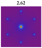
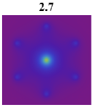
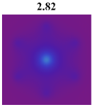
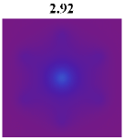
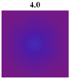
Figure 1: The single chain Green’s calculation of time-of-flight absorbtion picture for an ultra-cold Bose system in a triangular optical lattice for various $\widetilde{V}_{0}$.

V The visibility

However, the time-of-flight absorbtion picture can only provide us qualitative impression of the SF-MI phase transition. In addition, due to various experimental conditions, for instance the sensitivity of the detectors in the experimental setup, it is hard to compare the theoretical result of the time-of-flight pictures directly to experimental ones quantitatively. In order to winkle quantitative information out of the time-of-flight pictures, the so-called visibility Gerbier ; Gerbier2 has to be calculated. The visibility is defined as

$$\nu=\frac{n_{\rm max}-n_{\rm min}}{n_{\rm max}+n_{\rm min}},$$ (40)

From Eq.(37), it is easy to find out that $n_{\rm max}$ takes place at $(0,4\pi/(\sqrt{3}a))$ and $(2\pi/a,2\pi/(\sqrt{3}a))$ and other four equivalent points in the momentum space while $n_{\rm min}$ is at $(2\pi/(\sqrt{3}a),2\pi/a)$ , $(4\pi/(\sqrt{3}a),0)$, and other four equivalent points. All these points have the same distance from the original point, hence at these points the Wannier function $w({\bf k})$ takes the same value, thus the visibility is solely determined by the correlations at these points. The theoretical result as well as the experimental data taken from Ref.[sengstock, ] are plotted in Fig.2a.

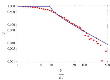
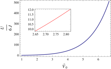
Figure 2: (a) The visibility of the interference pattern against $U/(6J)$. The solid blue line is the theoretical result from Eq.(40) and the red dots are from the experimental observation sengstock . (b) The dependence of $U/(6J)$ on $\widetilde{V}_{0}$.

From Fig.2a, it is easy to see that our analytical result shows that the visibility of the interference peaks of the system drops dramatically fast in the region of $10\leq\widetilde{V}_{0}\leq 12$. In Fig.2b, We plot the dependance of $U/(6J)$ on $\widetilde{V}_{0}$, the corresponding range of $\widetilde{V}_{0}$ is from 2.65 to 2.82, as can be seen in the inset of Fig.2b. The experimental estimation is that the corresponding region is from 3.5 to 4. There is roughly a 20% deviation between our analytical result and the experimental data, this is understandable: first, our calculation is a sort of mean-field result; second, during the calculation of $J$ and $U$, the Gaussian approximation of the Wannier function is adopted. Nevertheless, our theoretical prediction is in a reasonable agreement with the experimental data. Moreover, from the figure of visibility, we see that the visibility is non-zero far deep inside the Mott state, this is due to the short-range coherenceGerbier2 in Mott insulator.

VI Discussion

In conclusion, by treating the hopping parameter in Bose-Hubbard model as a perturbation, with the help of the re-summed Green’s function method and cumulants expansion, the momentum distribution function of the ultra-cold Bose system in triangular optical lattice is calculated analytically. By utilizing it, the time-of-flight absorption picture is plotted and the corresponding visibility is determined. The comparison between our analytical results and the experimental data from Ref.[sengstock, ] exhibits a qualitative agreement.

As we have seen in the discussion of the paper, this systematic approach can in principle be extended to regime beyond mean-field theory by adding loop diagrams, more precise expressions of Wannier function may be adopted to improve the accuracy of the analytical result. Moreover, the method presented here can not only be used to investigate homogeneous cold atomic system, but also can be used to systems with nearest neighbor repulsive interactions. Ultra-cold Bose gas on a triangular optical lattice accompanied by nearest neighbor repulsive interaction would exhibit geometrical frustration effect, hence our present work may shed some new light in this field.

References

- (1) M. Greiner, O. Mandel, T. Esslinger, T. W. Hänsch, and I. Bloch, Natrue(London) 415, 39 (2002).
- (2) I. Bloch, J. Dalibard, and W. Zwerger, Rev. Mod. Phys. 80, 885 (2008).
- (3) M. Lewenstein, A. Sanpera, V. Ahufinger, B. Damski, A. S. De, and U. Sen, Adv. Phys. 56, 243 (2007).
- (4) C. Becker, P. Soltan-Panahi, J. Kronjäer, S. Döscher, K. Bongs, and K. Sengstock, NJP 12, 065025 (2010).
- (5) J. Struck, C. Ölschläger, R. Le Targat, P. Soltan-Panahi, A. Eckardt, M. Lewenstein, P. Windpassinger, and K. Sengstock, Science 333, 996 (2011)
- (6) A. Eckardt, P. Hauke, P. S. Parvis, C. Becker, K. Sengstock and M. Lewenstein, Europhys. Lett. 89, 10010 (2010).
- (7) Z. Lin, J. Zhang, and Y. Jiang, Phys. Rev. A 85, 023619 (2012)
- (8) F.E.A. dos Santos and A. Pelster, Phys. Rev. A 79, 013614 (2009); B. Bradlyn, F. E. A. dos Santos and A. Pelster, Phys. Rev. A 79, 013615 (2009).
- (9) N. Elstner and H. Monien, Phys. Rev. B 59, 12184 (1999); N. Teichmann, D. Hinrichs, and M. Holthaus, Europhys. Lett. 91, 10004 (2010)
- (10) M. Greiner, I. Bloch, O. Mandel, T. W. Hänsch, and T. Esslinger, Phys. Rev. Lett. 87, 160405 (2001).
- (11) M. Köhl, H. Moritz, T. Stöferle, K. Günter, and T. Esslinger, Phys. Rev. Lett. 94, 080403 (2005).
- (12) W. Metzner, Phys. Rev.B 43, 8549 (1993).
- (13) M. Ohliger, Diploma thesis, Free University of Berlin, 2008, http://users.physik.fu-berlin.de/ ohliger/Diplom.pdf
- (14) D. Jaksch, C. Bruder, J. I. Cirac, C. W. Gardiner, and P. Zoller, Phys. Rev. Lett. 81, 3108 (1998).
- (15) P.B. Blakie, C.W. Clark, J. Phys. B 37, 1391 (2004)
- (16) V. A. Kashurnikov, N. V. Prokof ev, and B. V. Svistunov, Phys. Rev. A 66, 031601(R)(2002).
- (17) D. van Oosten, P. van der Straten, and H.T.C. Stoof, Phys. Rev. A 63, 053601 (2001)
- (18) M. Peskin and D. Schröder,An Introduction to Quantum Field Theory (Westview Press, Boulder, 1995).
- (19) A. Hoffmann and A. Pelster, Phys.Rev.A 79, 053623 (2009).
- (20) F. Gerbier, A. Widera, S. Föling, O. Mandel, T. Gericke, and I. Bloch, Phys. Rev. A 72, 053606 (2005).
- (21) F. Gerbier, A.Widera, S. Föling, O. Mandel, T. Gericke, and I. Bloch, Phys. Rev. Lett. 95, 050404 (2005).