Manifestation of Resonance-Related Chaos in Coupled Josephson Junctions

Abstract

Chaotic features of systems of coupled Josephson junctions are studied. Manifestation of chaos in the temporal dependence of the electric charge, related to a parametric resonance, is demonstrated through the calculation of the maximal Lyapunov exponent, phase-charge and charge-charge Lissajous diagrams and correlation functions. The number of junctions in the stack strongly influences the fine structure in the current voltage characteristics and a strong proximity effect results from the nonperiodic boundary conditions. The observed resonance-related chaos exhibits intermittency over a range of conditions and parameters. General features of the system are analyzed by means of a linearized equation and the criteria for a breakpoint region with no chaos are obtained. Such criteria could clarify recent experimental observations of variations in the power output from intrinsic Josephson junctions in high temperature superconductors.

I Introduction

Systems of coupled Josephson junctions (JJs) are prospective objects for superconducting electronics and therefore continue to be the subject of intense investigations.kleiner92 ; kadowaki ; krasnov11 ; savelev10 ; ozyuzer ; tachiki09 ; wang10 ; lin11 ; koshelev10 Intrinsic Josephson effects – tunneling of Cooper pairs between superconducting layers inside of strongly anisotropic layered high temperature superconductors (HTSCs) – provide an opportunity to model HTSCs as systems of coupled intrinsic Josephson junctions (IJJs) and an effective way to investigate nonlinear effects and non-equilibrium phenomena in HTSCs. Intrinsic tunneling is a powerful method for the study of the nature of high temperature superconductivity, transport along a stack of superconducting layers, and the physics of vortices. It also plays an important role in determining the current-voltage characteristics (CVCs) of tunneling structures based on HTSCs and the properties of vortex structures in these materials.

Parametric resonance in coupled JJs demonstrate a series of novel effects predicted by numerical simulations.sg-prb11 In comparison with the single junction, the system of coupled JJs has a multiple branch structure in its CVCs. The outermost branch of the CVCs has a breakpoint (BP) and a breakpoint region (BPR) before a transition to another branch, caused by parametric resonance.sm-prl07 The BP current characterizes the resonance point at which a longitudinal plasma wave (LPW) is created. It was demonstrated that the CVC of the stack exhibits a fine structure in the BPR.sms-prb08 The breakpoint features were predicted theoreticallysm-sust07 and recently observed experimentally.iso-apl08 A breakpoint region also appears in numerical simulations performed by other authors.machida99

The physics of IJJs, which are nonlinear systems, cannot be completely understood without the investigation of their chaotic features. Parametric instabilities are common phenomena in one-dimensional arrays of Josephson junctions. For example, a one-dimensional parallel array of $N$ identical Josephson junctions was studied by discrete sine-Gordon equation (also known as Frenkel-Kontorova model) in Ref.watanabe95, . The parametric instabilities were predicted by theoretical analysis and observed experimentally. In particular, the novel resonant steps related to the parametric instability were found in the current voltage characteristics of discrete Josephson ring. It was verified experimentally that such steps occur even if there were no vortices in the ring. A long Josephson junction is also often considered as a one-dimensional parallel array of $N$ identical Josephson junctions. An experimental testing of the parametric instability in IJJ would clarify the generic feature of one-dimensional parallel and series array models and the role played by resonance related chaos in these systems.

The chaotic features of IJJs in HTSCs are also of great interest due to the observed powerful coherent THz radiation from such systems.ozyuzer Broadly tunable sub-terahertz emission was found in the CVC near the switching point from the outermost branch to inner branches, and also from inner branches.kadowaki We stress that this is the same region in the CVCs where the BP and BPR were observed. Recently, for example, coherent THz radiation has been measured experimentally and was associated with a “bump” structure corresponding to the same part of the CVCs.ozyuzer12 ; benseman Obviously, the chaos in IJJs could strongly effect their radiation properties, because the transition to the chaotic state may inhibit the coherent radiation from IJJs. Therefore, detailed investigations of such transitions in real systems are very important. This situation makes the phase dynamics and the investigation of chaos in intrinsic JJs, near the BPR of the CVCs, an urgent problem.

In an early study of the rf current driven Josephson junction it was found that, depending on the amplitude of the rf current, the system would develop a chaotic character.Huberman80 ; Kautz81 ; Kautz85a ; Kautz85b It was also shown that the onset of chaos as a function of frequency correlated with the function that indicated infinite gain, also as a function of frequency, for the unbiased parametric amplifier.pedersen More recently the importance of chaos in IJJs, and its effects on the CVCs and the Shapiro steps in these systems, was stressed in Refs. irie03, ; scherbel04, .

In a further comprehensive study, the critical behavior of the dynamical equation, in the sense of how it goes from regular to chaotic, was investigated.tomas It was discovered that the critical behavior is that of the circle map. Here, in the subcritical state, the resonances are separated by quasi-periodic orbits (i.e. having irrational winding number), whereas in the supercritical state the dynamics is composed of chaotic jumps between resonances. The chaos appears to be the result of the overlap of resonances.mogens

In a similar study, the interaction of the Josephson junction with its surroundings was considered by coupling it in parallel with an RLC circuit, modeling a resonant cavity.borcherds The chaotic nature develops through the familiar period doubling sequence of bifurcations. Other studies exist that try to understand the irregular response of dissipative systems driven by external sources when such behavior is interleaved by the synchronized motion (Shapiro steps). This so called intermittent chaos is modeled by a random walk between the two neighboring steps that have become unstable. It is shown that the power spectrum of the voltage correlations has a broadband background characterizing the chaotic solution.benjacob It may be noted that a similar random walk model has been developed to explain the phase synchronization of chaotic rotators.osipov02

Interesting features of chaos, chaos control and chaotic synchronization in Josephson junction arrays (JJAs) and shunted JJ models have been described in Refs. ri11, ; feng10, ; whan96, ; basler95, ; zhou09, ; hassel06, ; bhagavatula94, ; chernikov94, . JJAs attract much attention due to their perspective as high precision voltage standards and, as mentioned earlier, high power coherent THz sources. Output power of a single junction is extremely low (typically 10 nW), but much higher output power can be obtained by using JJAs. Chaos and nonlinearity in JJAs have been described in Refs. basler95, ; zhou09, . In particular, Basler et al.basler95 reported on the theory of phase locking and self-synchronization in a small JJ cell by using the resistively shunted junction (RSJ) model and Hassel et al.hassel06 studied self-synchronization in distributed Josephson junction arrays. Features of spatiotemporal chaos in JJAs composed of RSJs were numerically investigated by Bhagavatula et al.bhagavatula94 Chernikov and Schmidtchernikov94 demonstrated that when four or more JJs are globally coupled by a common resistance, the system exhibits adiabatic chaos. Direct calculation results zhou09 showed that phase locking and chaos coexist when there are three junctions in the JJA. In Ref. ri11, chaos, hyperchaos and controlling hyperchaos in a JJA were investigated. The numerical results show that chaos and hyperchaos states can coexist in this array of two shunted JJs, independently of whether or not the original states of the junctions are chaotic.

Although there have been recent reports on the chaotic behavior in JJs, such as Ref. ri11, , there are relatively few detailed investigations of chaotic behavior in closely-related phenomenological models such as, the capacitively-coupled model (CCJJ),koyama96 the resistive-capacitive shunted model (RCSJJ),buckel ; whan96 or the capacitively coupled Josephson junction model with diffusion current (CCJJ+DC)sms-physC06 ; machida00 of the present work. Specifically, the chaotic features at the parametric resonance have not been investigated before.

In this paper, we study the phase dynamics in coupled Josephson junctions. A resonance-type chaos related to the parametric resonance in this system is demonstrated. The origin of chaos is related to the coupling between junctions based on the fact that the superconducting layers (S-layers) are in the nonstationary nonequilibrium state due to the injection of quasiparticle and Cooper pairs.koyama96 ; ryndyk-prl98 We present results on a chaotic mode which is due to the coupling between junctions and a parametric resonance in coupled JJs. This mode cannot be observed in case of a single JJ. Creation of a LPW and its interplay with a discrete lattice of superconducting layers produces a rich dynamic behavior, including, for example, intermittency. We use different methods to investigate this dynamics, including correlation functions and Lyapunov exponents. Results for stacks with different numbers of JJs, in which LPWs with different wave numbers are exited, give interesting information on certain features of the fine structure within the BPR of the CVCs. The influence of the boundary conditions on the chaotic part of the fine structure leads to the manifestation of a strong proximity effect in IJJs. Transitions between chaotic and regular behavior in BPR are predicted. Transitions from the chaotic state to both a regular LPW state and a traveling wave mode are demonstrated. Finally some general features of the system are analyzed and the conditions and parameters leading to a BPR with no chaos are found.

The paper is organized in the following way. In Section II we introduce the coupled sine-Gordon equation, used for numerical simulations, and discuss the boundary conditions and numerical procedures. We briefly describe the method for calculating the Lyapunov exponent. Section III is devoted to the study of the resonance-related chaos produced in the temporal dependence of the electric charge, and this is demonstrated through the calculation of the maximal Lyapunov exponent, phase-charge and charge-charge Lissajous diagrams and correlation functions. We also provide examples of the manifestation of related chaotic features in the correlation functions and polar diagrams. The effect of the number of junctions in the stack is considered in Sec. IV. Nonperiodic boundary conditions and the proximity effect in coupled JJs are discussed in Sec. V. We show the occurrence of transitions from chaotic to regular behavior in Sec. VI. To clarify the chaotic features in coupled JJs, we analyze the linearized equation for phase differences in Sec. VII, and discuss the question concerning the region of instability at chaotic boundary. In Sec. VIII we demonstrate the parametric resonance region without chaotic behavior. Conclusions follow in Sec. IX.

II Model and method

High-Tc superconductors have a layered crystal structure and strong anisotropy. A model of multilayered Josephson junctions, which has an alternating stack of superconducting and insulating layers, is sufficient to describe the electronic properties of these systemsmatsumoto99 . In the present model we assume that the physical quantities are spatially homogeneous on each layer. This assumption is applicable in cases of no applied magnetic field and for a small sample size in the $ab$-direction, i.e. for the intensively developing research field known as the physics of Josephson nanojunctions, where the length of the Josephson junctions is smaller than the Josephson penetration length. One-dimensional models with coupling between junctions do capture the main features of real IJJs, like hysteresis and branching of the current voltage characteristics, and thus help to improve the understanding of their physics. An interesting and very important fact is that the 1D models can also be used to describe the properties of a parallel array of Josephson junctions, which is often considered as a model for long Josephson junctions. The experiments and theoretical studies on the propagation of Josephson fluxons and electromagnetic waves in parallel arrays of Josephson junctions were presented in Refs.pfeiffer06; pfeiffer08. Their experimental data demonstrate a series of resonances in the current voltage characteristics of the array and were analyzed using the discrete sine-Gordon model and an extension of this model which includes a capacitive interaction between neighboring Josephson junctions.

To simulate the CVCs of intrinsic Josephson junctions in high temperature superconductors we investigate the phase dynamics within the framework of the CCJJ+DC model. ryndyk-prl98 ; machida00 ; sms-physC06 In this model the dynamical equations are given by,

$$\frac{{\textrm{d}}V_{l}}{{\textrm{d}}t}=I+I_{n}-\sin\varphi_{l}-\beta\frac{{\textrm{d}}\varphi_{l}}{{\textrm{d}}t},$$ (1a)

$$\frac{{\textrm{d}}\varphi_{l}}{{\textrm{d}}t}=V_{l}-\alpha(V_{l+1}+V_{l-1}-2V_{l}).$$ (1b)

Here $V_{l}\equiv V_{l+1,l}$ is the voltage difference between the $(l+1)$th and $l$th S-layers, and the gauge-invariant phase difference $\varphi_{l}$ between adjacent S-layers is given by $\varphi_{l}(t)=\theta_{l+1}(t)-\theta_{l}(t)-\frac{2e}{\hbar c}\int^{(l+1)d}_{ld+s}{\rm d}zA_{z}(z,t)$, where $\theta_{l}$ is the phase of the order parameter (i.e. phase of the macroscopic wave function of the superconductor) in the $l$th S-layer of thickness $s$, $A_{z}$ is the vector potential in the barrier of thickness $D$, and $d=s+D$ is the period of the lattice. In the above equations, $\alpha$ and $\beta$ are the coupling constant and dissipation parameter, respectively. Time $t$ is normalized to the inverse plasma frequency $\omega^{-1}_{p}$ (with $\omega_{p}^{2}=2eI_{c}/\hbar C$, and $C$ denoting the junction capacitance), the voltage differences $V_{l}$ are normalized to $V_{0}=\hbar\omega_{p}/(2e)$, and the bias current $I$ and added noise current $I_{n}$ are normalized to the critical current $I_{c}$. The role of the added noise current ($I_{n}\sim 10^{-8}$) has been discussed previously.sm-sust07 We solve this system of dynamical equations for stacks with various numbers ($N$) of JJs.

The system of Eqs. (1) can also be written in the form

$$\frac{{\rm d}^{2}\varphi_{l}}{{\rm d}t^{2}}=\sum_{l^{\prime}}\,A_{ll^{\prime}}\left[I+I_{n}-\sin\varphi_{l^{\prime}}-\beta\frac{{\rm d}\varphi_{l^{\prime}}}{{\rm d}t}\right]$$ (2)

where, for nonperiodic boundary conditions (BCs), the matrix $A$ has the form

$$A=\begin{pmatrix}1+\alpha G&-\alpha&0&...&&&\\ -\alpha&1+2\alpha&-\alpha&0&...&&\\ 0&-\alpha&1+2\alpha&-\alpha&0&...&\\ ...&...&...&...&...&...&...\\ &&&...&0&-\alpha&1+\alpha G\end{pmatrix}$$ (3)

Here $l$ and $l^{\prime}$ run over the $N$ junctions, $\beta_{c}=\omega_{p}^{2}R^{2}C^{2}$ is the McCumber parameter, and $G=1+\gamma$, $\gamma=s/s_{0}=s/s_{N}$, where $s$, $s_{0}$ and $s_{N}$ are the thicknesses of the middle, first, and last $S$ layers, respectively. According to the proximity effect, the thicknesses of the first and last layers are assumed to be thicker than the middle layers inside the stack. So, for the nonperiodic boundary BCs, the equations for the first and last layers in Eq. (2) are different from those of the middle layers.koyama96 ; matsumoto99 For periodic BCs the matrix $A$ has the form

$$A=\begin{pmatrix}1+2\alpha&-\alpha&0&...&&&-\alpha\\ -\alpha&1+2\alpha&-\alpha&0&...&&\\ 0&-\alpha&1+2\alpha&-\alpha&0&...&\\ ...&...&...&...&...&...&...\\ -\alpha&&&...&0&-\alpha&1+2\alpha\end{pmatrix}$$ (4)

Using the Maxwell equation $\varepsilon\varepsilon_{0}\textrm{div}{\vec{E}}=Q$, where $\varepsilon$ is the dielectric constant of the insulating layers and $\varepsilon_{0}$ is the permittivity of free space, we express the charge density in the $l$th S-layer as

$$Q_{l}=Q_{0}\alpha(V_{l+1}-V_{l}),$$ (5)

where $Q_{0}=\varepsilon\varepsilon_{0}V_{0}/r_{D}^{2}$ and $r_{D}$ is the Debye screening length. In all our calculations the CVCs and time dependence of the charge oscillations in the S-layers are simulated at $\alpha=1$. The system not very sensitive to the value of the coupling parameter. Further details concerning numerical simulations of the CVCs and the electric charge can be found in Refs. smp-prb07, ; shk-prb09, ; matsumoto99, .

The usual test for chaos in a system is through the calculation of the largest Lyapunov exponent (LE).chaosb The general idea is to follow two nearby trajectories and to calculate their average logarithmic rate of separation. Whenever the two trajectories get too far apart, one of them has to be moved back to the vicinity of the other, along the line of separation. A conservative procedure is to do this at each iteration.

In this paper we solve the system of Eqs. (1), using a fourth-order Runge-Kutta method, to find the $V_{l}$ and $\varphi_{l}$. To this end we choose the time domain $T_{f}$ and time step $T_{p}=T_{f}/m$, such that $t_{j}=jT_{p}$, for $j=0,\ldots,m$. In order to calculate the largest LE, at fixed current $I$, we first integrate the system for a time $T_{i}$, until all transients have decayed. Then, starting from an arbitrary small initial separation vector ${\vec{d}}_{j}\equiv(\Delta V(t_{j}),\Delta\varphi(t_{j}))$, we advance both systems by one time step and calculate the new separation ${\vec{d}}_{j+1}\equiv(\Delta V(t_{j+1}),\Delta\varphi(t_{j+1}))$, where $\Delta\varphi_{l}(t_{i})=\varphi^{\prime}_{l}(t_{i})-\varphi_{l}(t_{i})$ and $\Delta V_{l}(t_{i})=V^{\prime}_{l}(t_{i})-V_{l}(t_{i})$. The Lyapunov exponent for this step is defined by

$$LE_{i}=\frac{1}{T_{p}}\ln\frac{\|{\vec{d}}_{j+1}\|}{\|{\vec{d}}_{j}\|},$$ (6)

where $\|{\vec{d}}_{j}\|=[\sum_{l=1}^{N}(\Delta\varphi_{l}(t_{j}))^{2}+(\Delta V_{l}(t_{j}))^{2}]^{1/2}$. In order to avoid cumulative numerical round-off errors, due to the expected exponential changes in separation, the separation vector is rescaled after each step in time, i.e. we set ${\vec{d}}_{j+1}\equiv(\|{\vec{d}}_{j}\|/\|{\vec{d}}_{j+1}\|){\vec{d}}_{j+1}$, before advancing to the next step. This procedure is iterated over the rest of the time domain at fixed current. Finally we take the average of all the $LE_{j}$ to find the Lyapunov exponent

$$LE(I)=\frac{1}{m-k}\sum_{j=k}^{m-1}LE_{j}\,.$$ (7)

where $t_{k}=kT_{p}=T_{i}$. By changing the current in small steps (${\rm d}I$), and repeating the above procedure for each value of current, the $LE$ is obtained as a function of current. Typically, except where noted, we have used $T_{i}=50$, $T_{f}=25000$, $m=5\times 10^{5}$, and ${\rm d}I\leq 5\times 10^{-4}$. Additional details concerning the LE calculation can be found in Refs. chaosb, ; chaos1, ; chaos2, .

III Indications of chaos in the BPR for a system of coupled JJs

The CVCs of coupled JJs has a multiple branch structure. Here we concentrate on the outermost branch only. The system of coupled JJs exhibits a parametric resonance which is reflected in the CVC as a breakpoint. In stacks with odd numbers of junctions a breakpoint region, with a fine structure corresponding to the width of the parametric resonance, is observed. A study of the fine structure in the BPR gives one enough reason to look for chaos in the dynamics of a stack. Its manifestation depends strongly on the parameters of the system. Here we present some examples and methods, which might be used for demonstration and investigation of the chaotic features of coupled JJs.

First, we consider a stack of 9 JJs using periodic BCs with $\beta=0.2$. In Fig. 1, the Lyapunov exponent and outermost branch of CVCs, as functions of current, are compared with the charge oscillation in the 8th S-layer, as a function of time and current.

To calculate the voltages $V_{l}(I)$ at each point of CVC (i.e. for each value of $I$), we simulate the dynamics of the phases $\varphi_{l}(t)$ by solving the system of equations (1) using the fourth-order Runge-Kutta method with a time step $T_{p}$. After simulation of the phase dynamics we calculate the dc voltages on each junction by averaging over a chosen time domain. After completing the voltage averaging for the fixed bias current $I$, the bias current is increased or decreased by a small amount $dI$ (bias current step) in order to calculate the voltages in all junctions at the next point of the CVC. We use the distribution of phases and their derivatives at the end of the time domain of previous point as the initial distribution for calculating the next point. In this manner the dependence of charge on current ‘includes’ the time dependence of each current step.

In the inset we illustrate the position of the BPR on the outermost branch of the CVCs.

Figure 1: (Color online) Lyapunov exponent and CVC, as functions of current, with the charge oscillation in $Q_{8}$ (the charge in the 8th S-layer) as a function of time. Inset demonstrates the position of the BP on the outermost branch of the CVCs.

As one can observe, there are two distinct regions: $LE=0$ and $LE>0$. The case $LE>0$ strictly indicates that the system is chaotic over the approximate current interval of $(0.5620,0.5536)$, while $LE=0$ indicates marginal stability for the system elsewhere. Both the CVCs and charge oscillations show chaotic features which coincide with $LE>0$.

Second, we study the correlations in superconducting currents in the neighboring Josephson junctions, and charge correlations in neighboring superconducting layers. This allows us to further demonstrate the observed chaotic features in CVC. The charge-charge correlation functions for neighboring layers are given by

$$C^{c}_{l,l+1}(I) = \left<Q_{l}(t)Q_{l+1}(t)\right>$$

$$= \lim_{T_{f}\rightarrow\infty}\frac{1}{T_{f}-T_{i}}\int_{T_{i}}^{T_{f}}{Q_{l}(t)Q_{l+1}(t){\rm d}t},$$

where $l$ is the layer number and $T_{i}$ is the initial time for the averaging procedure. Figure 2 presents the results of calculations for the cases $l=2$ and $l=7$, for the same stack of nine JJs. The negative sign of $C^{c}_{l,l+1}$ is due to the fact that a LPW with wave number $k=8\pi/(9d)$ is created. This wave number is close to the $\pi$-mode, for which the charge on neighboring layers differs in sign, and hence the product of positive and negative charges produces a negative sign (cf. Sec. IV).

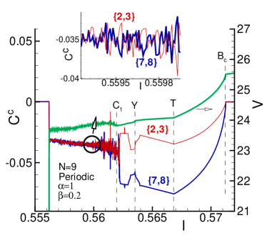
Figure 2: (Color online) The charge correlation functions $C^{c}_{l,l+1}=\left<Q_{l}(t)Q_{l+1}(t)\right>$ for $l=2$ (labeled by 2,3) and $l=7$ (labeled 7,8) for the stack with nine IJJ as a function of the bias current. CVC is also shown (and labeled by an arrow). A chaotic part of the BPR (encircled) is enlarged in the inset.

Here the expected feature of the correlation functions in the chaotic region is confirmed: at the transition to chaotic behavior (point $C_{1}$), the values of all correlation functions approach each other, i.e. $\left<Q_{l}(t)Q_{l+1}(t)\right>=\left<Q_{l}(t)\right>\left<Q_{l+1}(t)\right>$. Thus, within the chaotic region, all correlations are lost. To demonstrate the character of the correlation function, we enlarged a region in the chaotic part of the BPR in the inset to Fig. 2. We see that both correlation functions $C_{2,3}$ and $C_{7,8}$ show a similar variation with current, in agreement with the Lyapunov exponent.

Third, manifestations of the chaotic behavior can also be demonstrated by phase-charge diagrams. To do so, we record the time dependence of the phase difference across the chosen junction and electric charge in the chosen S-layer at a given bias current. Figure 3 shows such a phase-charge diagram: the variation of the absolute value of charge in the first superconducting layer $Q_{1}$ with the phase difference $\varphi_{1}$ across the first JJ of the stack.

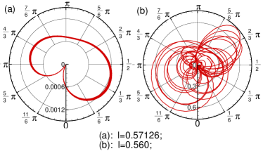
Figure 3: (Color online) The phase-charge diagram. It shows the absolute value of the charge on the first superconducting layer (radial coordinate), versus the phase difference across the first junction at two values of bias current: (a) $I=0.57126$ and (b) $I=0.56000$.

This is a Lissajous figure, showing that the motion at $I=0.57126$ is qualitatively different from that at $I=0.560$, thus providing additional evidence of chaos in this part of the CVCs.

IV Effect of the number of junctions in the stack

We next study the behavior of the stacks as a function of the number of junctions. To clarify this effect, we first discuss the parametric resonance features in the stacks with even and odd numbers of JJs.

In the stacks with an even number of junctions and periodic BCs, at $\beta=0.2$, a LPW with wave number $k=\pi$ ($\pi$-mode) is created, so that its wavelength $\lambda=2d$ satisfies the commensurability condition $L=n\lambda$.smp-prb07 Here $L=Nd$ is the length of the stack, and $d$ is the period of the lattice. In this case a fine structure in the BPR is absent and the transition from the outermost branch to another one is observed after a sharp (exponential) increase of charge in S-layers. Also, the value of the breakpoint current is the same for all stacks with an even number of junctions. The sharp increase of charge in the S-layers happens in a very narrow interval of the bias current. For example, in a simulation of the CVC in a stack with $N=10$ and a current step of $10^{-4}$, the interval is (0.5771, 0.5767) in which the increase of charge is of about 7 orders of magnitude.

In the stacks with an odd number of junctions the wave number of the LPW is $k=(N-1)\pi/(Nd)$ which approaches $k=\pi/d$ as $N$ increases. The value of the BP current is limited by its value at $k=\pi$, and the width of the BPR decreases with increasing $N$.smp-prb07 With an odd number of junctions in the stack, the sharp increase of the charge accompanies the BP but then, before transition to another branch, a wide BPR exists.sms-prb08 The origin of it is explained by the fact that the wavelength of LPW does not satisfy the commensurability condition. The fine structure is related to the character of the charge oscillations in the superconducting layers sms-prb08 . A part of BPR reflects the chaotic behavior of the system, which is the main subject of our paper. Next we look at how $N$ affects the structure of BPR. As mentioned above, the study of the correlation of charge on neighboring S-layers is a powerful tool to investigate the dynamics of charge in coupled JJs, within the BPR.shk-prb09 Here we use it to demonstrate the effect of the number of junctions on the structure of the BPR.

For the periodic BCs the number assigned to a junction is merely a label. However, in order to compare the correlation functions between stacks with different numbers of junctions, in different simulations, it is useful to use a specific layer as reference. In the parametric resonance region the phase dynamics in the coupled system of JJs singles out such specific layers, namely, if a node of the charge standing wave coincides with the layer, then the charge on that layer is close to zero. Therefore we number the correlation functions according to their distance from such specific layers, as shown in Fig. 4.

Figure 4: (Color online) Formation of the charge correlation functions in a periodic stack of 9 IJJs. The numbers count the layers in the stack.

To reflect the symmetry of the correlation function relative to the chosen specific layer, we introduce the subscripts $+$ and $-$ on the correlation functions, as shown in Fig. 4. In this case the specific layer is number 4, and we have $C^{c}_{1+}=C^{c}_{4,5}$ and $C^{c}_{1-}=C^{c}_{3,4}$ and so on.

Figure 5 shows the part of the outermost branch of CVC in the BPR together with two correlation functions $C^{c}_{2+}$ and $C^{c}_{2-}$ for the stacks with 7, 9, 11 and 13 JJs with periodic BCs, at $\beta=0.2$.

Figure 5: (Color online) The CVC of the outermost branch in BPR together with correlation functions $C^{c}_{2+}$ and $C^{c}_{2-}$ for periodic stacks with different numbers of IJJs: (a) $N=7$; (b) $N=9$; (c) $N=11$; (d) $N=13$.

In each case the part around $B_{c}$ corresponds to the maximal increase of charge in the S-layers (c.f. the beginning of charge dependence in Fig. 2) and is characterized by a LPW frequency $\omega_{LPW}$. To distinguish different parts of BPR, we introduce the notation: $B$ for the beginning of the parametric resonance, $B_{c}$ for the BP of the CVC, $T$ and $W$ to indicate the appearance of low frequency charge modulations, and $C_{1}$ to separate the chaotic part of the BPR. The loops that are seen in the correlation functions to the left of $B_{c}$ (very clearly manifested for $N=13$), correspond to the charge dynamics on the specific layer in the regular part of the BPR and were discussed in Ref. shk-prb09, .

In the part $T-Y$ a modulation of the charge oscillations with low frequency appears.sms-prb08 The part $Y-C_{1}$ is the transition region between regular and chaotic behavior where a second low frequency is observed. The features in the transition region $Y-C_{1}$ relate to the specific behavior of the LPW with $k=(N-1)\pi/(Nd)$ in the stacks with different $N$. We found that the region after $C_{1}$ demonstrates the chaotic behavior of coupled system of Josephson junctions.

From Fig. 5 one can draw the following conclusion: The increase in $N$ increases the value of the breakpoint current, shifting the position of the BPR and decreasing the width of the BPR. As one can see, the increase in $N$ retains the main features of the BPR structure for the stacks with 7, 9, 11 and 13 junctions. Simulation of the time dependence of the charge in S-layers in these regions confirms the same character of the charge oscillations for all these stacks. The detailed features seen in the fine structure of the correlation functions, for the stacks with different numbers of junctions, and hence also different lengths, are related to the specific behavior of LPWs with different wave numbers. As will be discussed in Sec. VI, transitions from chaotic to regular and back can be observed clearly in, for example, Fig. 5(a), at $I\approx 0.556$.

Although the width of the BPR decreases with increasing $N$, the width corresponding to the chaotic behavior increases with increasing $N$. This fact is demonstrated in Fig. 6, where the LE as a function of $I$ is presented for stacks consisting of different numbers of junctions.

Figure 6: (Color online) Maximal Lyapunov exponents for periodic stacks with odd numbers of junctions $N$. Double arrows emphasize the increase in width of the chaotic region, relative to the BPR, as $N$ changes from $5$ to $15$.

We see that the chaotic part of the CVC with five junctions is significantly smaller that for $15$ junctions. This fact has been stressed by the double arrows shown in Fig. 6.

V Proximity effect

Contact of the stack of superconducting layers with a normal metal (electrodes) leads to the proximity effect: the superconducting regions are expected to penetrate into the electrodes. Due to the proximity the effective thicknesses of the superconducting layers at the edges of the stack, $s_{0}$ and $s_{N}$, are larger than the thicknesses, $s$, of the middle layers. As mentioned in connection with Eq. (3), this effect can be taken into account by variation of the parameter $\gamma$ in the nonperiodic BCs.matsumoto99 Therefore, in this section, we consider briefly the influence of $\gamma$ on the chaotic behavior of the CVC and correlation functions.

The CVC and correlation function, $C^{c}_{5}=C^{c}_{5,6}(I)=\left<Q_{5}(t)Q_{6}(t)\right>(I)$, at $\gamma=0,0.5\mbox{ and }1$ are presented in Fig. 7 for a stack of 9 junctions. In this case, the LPW with $k=(N-1)\pi/N$ is created at the breakpoint for all stacks, with an even and odd number of junctions and with $\beta=0.2$.smp-prb07 Figure 7(a) shows the case $\gamma=0$. As we see, the main features of the CVC and the correlation functions are coincident. Within the chaotic region there appears to be some regions with regular oscillations, marked by arrows. Figure 7(b) clearly shows two such regions in CVC and in the correlation function at $\gamma=0.5$.

Figure 7: (Color online) The CVC and correlation function ${C^{c}}_{5}$ in the BPR for the stack with 9 IJJ at (a) $\gamma=0$; (b) $\gamma=0.5$; (c) $\gamma=1$. Inset to (c) shows an enlarged view of the encircled area near the BP.

With increasing $\gamma$ the width of the BPR is decreased, especially the $B_{c}-T$ region, which becomes very small by the time $\gamma=1$. An enlarged view of this small region is shown in the inset to Fig. 7(c).

Taking into account the proximity effect further emphasizes the influence of the number of junctions in the stack. In particular, for $\gamma=1$, the entire BPR becomes chaotic as $N$ increases beyond about 15. This result is presented in Fig. 8, where the CVC of the outermost branch together with LE are compared for $N=7$ and $N=15$.

Figure 8: (Color online) CVC of the outermost branch for stacks with (a) $N=7$ and (b) $N=15$ JJs together with the LE at $\gamma=1$.

We see that in the case $N=15$, the LE becomes positive practically just after the breakpoint. In view of these results we predict that the proximity effect will have a strong influence on the fine structure of the BPR in the CVC of real junctions.

VI Intermittency in CVC and correlation functions

As we have seen in Fig. 7, there are some regular regions within the chaotic parts of the CVC and correlation functions, and so transitions exist from chaotic to regular behavior and back. This is known as intermittency in dynamical systems with chaotic dynamics.roberto85 ; strogatz94 Now, for the first time, we demonstrate such intermittency for the resonance related chaos in systems of coupled JJs. Many such transitions can be seen in Fig. 9, where we present results of a high precision calculation of the LE together with the CVC for a stack of 9 junctions, using nonperiodic BCs, at $\gamma=0.5$. In this calculation $T_{i}=50$, $T_{f}=250000$, $m=5\times 10^{6}$ and ${\rm d}I=10^{-5}$.

Figure 9: (Color online) Intermittency is shown by windows of $LE=0$ inside the chaotic dynamics for a stack of 9 JJs with nonperiodic BCs. Arrows point to the respective scales for each curve and the dashed line shows the $LE=0$ axis. Double arrows show the correspondence between features of the CVC and the LE.

The regular regions seen in the CVC coinciding with $LE=0$. In particular the two largest intervals with $LE=0$ correspond to the current intervals $(0.5598,0.5600)$ and $(0.5573,0.5575)$, shown by double arrows. To better understand the nature of these transitions, the charge time dependencies in these regions should be considered. In future work it would also be of interest to calculate the full spectrum of Lyapunov exponents, which would allow one to distinguish between chaotic behavior (one positive exponent) and hyperchaotic behavior (more than one positive exponent).

To gain more information about the transitions we investigate the dependence of all the charge-charge correlation functions and the LE, on the bias current in the BPR. As the LE shows in Fig. 10, the absence of the charge correlations in different S-layers is a signature of the chaotic behavior. Since we are interested in the chaotic features, we have not labeled each curve by its corresponding correlation function. In Fig. 10 we see a restoration of correlations in the middle of the chaotic region for a stack with 13 JJs. All presented characteristics (Cc, CVC and LE) reflect this transition from the chaotic behavior to regular and back.

Figure 10: (Color online) Demonstration of the intermittency within the interval of bias current $0.5659<I<0.5565$ (shown by a double arrow) for the charge-charge correlation functions (Cc) and LE for a periodic stack of 13 junctions.

To stress the agreement between the correlation functions and LE, vertical dashed lines have been drawn in Fig. 10. We see that changes in the LE (small peaks on the LE curve) correspond exactly to changes in the charge correlations.

We have characterized one such transition from the chaotic to regular behavior as corresponding to a charge traveling wave state.sh-zhetp-l-12 As shown in Fig. 11, a transition from chaos to the traveling wave branch (TWB, dashed line) exists for the stack with 7 junctions, at $\beta=0.2$. This transition is encircled in the figure.

Figure 11: (Color online) Transition in the outermost branch (OB) to the traveling wave branch (TWB) in the CVC of the stack with 7 JJ. Inset above the curve demonstrates charge vs. time for S-layer at the transition point. Inset below the curve shows the charge-charge diagram for the neighbor S-layers in the chaotic region of the OB and in TWB.

We can see in the upper inset that the time dependence of charge in this region demonstrates a changing of character of the charge oscillations in S-layer. In the other inset (bottom right of Fig. 11) we have shown the Lissajous charge-charge diagram in the chaotic state and in the TWB. The diagram demonstrate the variation in time of the charges in two neighboring layers. The charge in the first S-layer, $Q_{1}$, is plotted along the $x$-axis, and the charge in the second S-layer, $Q_{2}$, is plotted along the $y$-axis. As we can see, the Lissajous charge-charge diagram presents an open trajectory for the chaotic region and a closed one for the TWB. Chaos in systems of coupled JJs can also be transformed to regular behavior by external irradiation. This is effected by adding a time dependent current to $I$ to the right hand side of Eq. (1), through the additional term, $A\sin(\omega_{R}t)$, where $A$ and $\omega_{R}$ are the amplitude and frequency of the microwave radiation. This result paves the way for experimental testing of the observed transitions from chaotic to regular traveling wave behavior. Detailed investigations of the effects of radiation on IJJs will be made in a future study.

VII Linearized Equation: Parametric Resonance

In this section we show that the linearized equation for the Fourier component $\delta_{k}$ of the phase difference $\delta_{l}=\varphi_{l+1}-\varphi_{l}$ can determine the region of instability of the coupled JJ states, and that together with calculation of the Lyapunov exponent, in the framework of the same equation, we can arrive at some important conclusions concerning the dynamics of this system. In particular, there is a region of parameter values corresponding to the parametric resonance without transition to the chaotic state. This conclusion is supported by the results of the investigation of the temporal dependence of the electric charge in S-layers and the correlation functions.

To investigate the instability region of coupled JJ states, corresponding to the outermost branch, we use the following linearized equation.sm-sust07 ; smp-prb07 ; sm-prl07 It can be obtained from Eq. (2) as,

$$\ddot{\delta}_{l}+(1-\alpha\nabla^{(2)})(\cos(\varphi)\delta_{l}+\beta\dot{\delta}_{l})=0,$$ (9)

by using the linear approximation $\sin(\varphi_{l+1})-\sin(\varphi_{l})\approx\delta_{l}\cos(\varphi)$, where $\varphi\simeq\Omega t=Vt/N$, $\Omega=V/N$ is the Josephson frequency, and $V$ is the total voltage across the stack. Use of the Fourier expansion $\delta_{l}(t)=\sum_{k}\delta_{k}e^{ikl}$, produces

$$\ddot{\delta_{k}}+\beta(k)\dot{\delta_{k}}+\cos(\Omega(k)t)\delta_{k}=0,$$ (10)

where $t$ is normalized to $\omega^{-1}_{p}(k)$, with $\omega_{p}(k)=\omega_{p}C_{\alpha}$, $\beta(k)=\beta C_{\alpha}$, $\Omega(k)=\Omega/C_{\alpha}$ and $C_{\alpha}=\sqrt{1+2\alpha(1-\cos(k))}$. In Eq. (9), we have used the discrete Laplacian $\nabla^{(2)}f_{l}=f_{l+1}+f_{l-1}-2f_{l}$.

The linearized equation  (10) demonstrates the instability region on the $\beta(k)-\Omega(k)$ diagram, which characterizes the parametric resonance in the coupled JJ.sm-prl07 This linear equation is similar to a damped Mathieu type equation, with its periodic coefficient, demonstrating parametric instability (resonance).mathieu

We calculate the LE for the dynamics dictated by the linearized equation (10), by the method described above, for the same system considered in Fig. 1. Three-dimensional results are presented in Fig. 12. In our calculations we have taken $m=300000$, $d\Omega(k)=0.005$ and $d\beta(k)=0.005$. Below, we consider different cross sections of this figure. The LE has positive values at small values of $\Omega(k)$ and $\beta(k)$) and is negative for large $\Omega(k)$ and $\beta(k)$). We also show the boundary between these regimes by the curve denoting $LE=0$, in Fig 13.

Figure 12: (Color online) Three dimensional picture of dependence of Lyapunov exponent versus $\Omega(k)$ and $\beta(k)$ given by equation (7). (a) The dependence of LE on $\Omega(k)$ at fixed $\beta(k)$; (b) The dependence of LE on $\beta(k)$ at fixed $\Omega(k)$.

To clarify the results presented in Fig. 12, we demonstrate two cross sections of it in the insets (a) and (b). Inset (a) shows the LE at constant value of dissipation parameter $\beta(k)=0.7$ as a function of $\Omega(k)$. We note that the $\Omega(k)$ is related to the voltage by Josephson relation $\Omega(k)={V}/{(NC(k))}$, i.e. $\Omega(k)$ is proportional to voltage. The dashed line shows $LE=0$. For large enough $\Omega(k)$, the LE is negative which points to regular dynamics in the system. For lower values of $\Omega(k)$ the behavior of the system is chaotic. Inset (b) shows the LE at constant value of voltage $\Omega(k)=0.7$ as a function of $\beta(k)$.

In Fig. 13 we show the cross section of Fig. 12 with $LE=0$ plane (solid line) together with the instability region (dashed line). Above the curve $LE=0$, the behavior of the system is regular, and below it, chaotic. The border of the instability region is related to the parametric resonance in the system. The region between these two curves determines the regular behavior showing parametric resonance.

Figure 13: (Color online) Lyapunov exponent (solid) and resonance region (dashed) in $\Omega(k)$-$\beta(k)$ plane. $\varepsilon$ denotes the width of regular region in direction of $\Omega(k)$ axis. The horizontal double dashed dotted line corresponds to the value $\beta(k)=0.9772$. A system with this value of $\beta(k)$ doesn’t touch the chaotic region. Below we demonstrate that chaotic part of BPR does not appear for this value of $\beta(k)$ (see Fig. 15).

Comparison of the Fig. 13 and Fig. 1 allows us to estimate the width of the regular region at fixed $\beta(k)$, and check the accuracy of linearization and approximations we have used to derive Eq. (10). From our definition of $\Omega(k)$, we have $\Delta V=NC_{k}\varepsilon$, where $\varepsilon=\Delta\Omega(k)$ denotes the width of regular region in direction of $\Omega(k)$ axis (see Fig. 13). In the case $k={8\pi}/{9}$ (the corresponding BPR in CVC for the 9 coupled JJs with $\beta=0.2$ is shown in Fig. 1) we find $C_{\alpha}=\sqrt{1+2\alpha(1-\cos(k))}=2.2$. Then $\beta(k)=\beta C_{\alpha}=0.44$. From Fig. 13 for this $\beta(k)$ we have $\varepsilon=0.071$ and $\Delta V=NC_{k}\varepsilon\approx 1.4$. As we can estimate from Fig. 1 the width of regular region is $\Delta V\approx 1.6$. So, the linearization and approximations used are accurate enough and there is a good agreement between results presented in Figs. 13 and 1.

VIII Parametric resonance region without chaotic behavior: case $\beta=0.6$

Let us now discuss in more detail the prediction which follows from Fig. 13; namely, that there is an interval of $\beta(k)$ values for each fixed $\Omega(k)$ corresponding to the BPR without chaotic behavior. To find $\beta$ which corresponds to a $\beta(k)$ in the discussed interval, we should know the wave number of the created LPW. We take an arbitrary value of $\beta(k)=0.9772$ in this interval. To determine the corresponding value of $\beta$ we first find the wave number of LPW which is created in this case at the resonance point. For this purpose we investigate, in Fig. 14, the $\beta$-dependence of the breakpoint current $I_{bp}$ (see details in Ref. sm-prl07, ) in Fig. 14. Inset shows the enlarged part of the figure where changes of the wave number $k$ of the LPW happen. We see that the value of $\beta=0.6$ corresponds to $k=4\pi/9$.

Figure 14: (Color online) Breakpoint current $I_{BP}$ and the jump current $I_{J}$ (where transition to another CVC branch occurs) versus $\beta$. Inset shows the enlarged part where changes of the wave number of LPW happen.

We examine our idea at $\beta=0.6$ to check if for the stack with 9 coupled JJ a chaotic region is absent, and to see the character of charge oscillations in the S-layers. According to the relation $\beta(k)=\beta C_{\alpha}$, the value of $\beta=0.6$ follows from that chosen in Fig. 13, namely $\beta(k)=0.9772$ and the LPW wave number $k={4\pi}/{9}$ because $C_{\alpha}=\sqrt{1+2\alpha(1-\cos(k))}=1.6287$.

In Fig. 15 we show the outermost branch in CVC of a stack of $N=9$ coupled JJs with periodic BCs, at $\beta=0.6$. Inset (a) to this figure shows the enlarged BPR. In this inset we see that the chaotic part of BPR does not appear. To stress the absence of the chaotic part in the BPR we also show the results for a system without noise ($I_{n}=0$) in Fig. 15. In this case the system behaves like a single JJ without a BPR in CVC. The curves before the parametric resonance region coincide.

Figure 15: (Color online) CVC of the stack with N=9 Josephson junctions at $\beta=0.6$ and periodic BC. Inset (a) demonstrates the enlarged part of BPR. Inset (b) shows electric charge on layers versus time.

To see the dynamics of the electric charge in the S-layers, we show the time variation of charge on one layer of a stack with 9 JJs with $\beta=0.6$ and periodic BCs in the inset (b) to Fig. 15. We see absolutely regular oscillations.

Finally, we look at the charge correlations in neighboring S-layers in a system without chaotic behavior in the parametric resonance region. As we know such a study is a powerful tool for the investigation of the dynamics of coupled JJsshk-prb09 . Results of calculations are presented in Fig. 16 which demonstrates the charge-charge correlation function (as defined in Sec. III) versus the bias current for neighboring layers in the stack with 9 coupled JJs at $\beta=0.6$. Here we are comparing the correlations within a specific stack, and so we use the usual notation for the correlation functions, i.e. $C^{c}_{l,l+1}\equiv\{l,l+1\}$.

Figure 16: (Color online) (a) Charge-charge correlation functions versus bias current for the stack with 9 junctions for $\beta=0.6$. Inset shows the charge distribution on S-layers at $I=0.845$. (b) Demonstration of correlation function pairing shown in (a).

We see that the behavior of the correlation functions reflects the behavior of the CVC in the BPR shown in Fig. 15, and corresponds to regular dynamics in the coupled JJs. The correlations in the oscillations of the charge in S-layers persist up to the transition to another branch in CVC. The inset to Fig. 16(a) shows the charge distribution on S-layers at $I=0.845$ and for the wave number $k={4\pi}/{9}$. In Fig. 16(b) we see that the correlation functions form pairs corresponding to the standing LPW. This pairing is demonstrated in Fig. 16(b), from which one can conclude that the 6th S-layer plays the role of the specific layer. In this case the charge on the 6th layer is non-zero, because the wavelength of the LPW is $\lambda=4.5d$ (not shown in Fig. 16(b)). Thus, the above analysis is a proof of concept for the existence of parameters leading to a BPR without chaos.

IX Conclusions

Physical properties of intrinsic Josephson junctions in high temperature superconductors continue to attract much attention due to the prospects they offer for superconducting electronics, in particular, as high power sources of coherent electromagnetic radiation in the THz region and high precision voltage standards. Applications would depend strongly on the chaotic properties such systems. Observed radiation spectra from IJJs are very complex and are temperature dependent. Transition of any junction in the stack to the chaotic state would lead to a loss of synchronization and coherent emission from the stack. The dissipation parameter (McCumber parameter) is itself temperature dependent, and this has to be taken into account when predicting the transition to the chaotic state in real systems.

Here we have studied chaotic features of coupled intrinsic Josephson junctions which might impact on their possible applications. Different manifestations of the chaotic behavior were seen in the temporal dependence of the electric charge in the superconducting layers, phase-charge and charge-charge Lissajous diagrams, Lyapunov exponent and correlation functions. We demonstrated that the number of junctions in the stack and the boundary conditions do influence on the chaotic part in the breakpoint region. Experimental testing of the above features may therefore expedite progress in their potential applications. The chaotic part of BPR increases with the number of junctions in the stack, relative to the regular part of the BPR, at nonperiodic BCs. Transitions between chaotic and regular behavior inside of the chaotic part of the breakpoint region were seen. It is anticipated that future developments in this direction of research may uncover new chaotic aspects in coupled JJs.

Our analysis of the general features of the system has uncovered the conditions and parameters that produce a breakpoint region without chaos. We have shown that for high enough values of dissipation parameter $\beta$ the chaotic part of breakpoint region does not exist. This is reminiscent of a single overdamped junction which lacks chaotic dynamics.gitterman10 We also arrived at the important prediction that the proximity effect should be expected to have a strong influence on the fine structure of the breakpoint region.

In order to better understand the nature of the intermittency in coupled JJs the charge time dependencies in these regions should be considered in future work. It may also be of interest to calculate the full spectrum of Lyapunov exponents, rather than only the maximal exponent, in order to distinguish between chaotic and (possibly) hyperchaotic behavior in these systems.

Presently there is renewed interest in phenomena related to the switching from the outermost branch to inner branches and transitions between inner branches. Recently, for example, powerful coherent THz radiation was observed experimentally and was associated with a “bump” structure in the same part of the CVC where the BPR was found.kadowaki ; benseman The recently observed broadly tunable sub-terahertz emission from internal branches of the CVCskadowaki stresses the importance of further investigations of the chaos related to these inner branches.

X Acknowledgments

Yu.M.S. thanks Paul Seidel, Elena Zemlyanaya and Ilhom Rahmonov for stimulating discussions and V. V. Voronov, V. A. Osipov for supporting this work. Support from the South Africa-JINR collaboration is also acknowledged. M. R. Kolahchi acknowledges support from the Institute for Advanced Studies in Basic Sciences, Zanjan, Iran. A.E.B. acknowledges that this work is based upon research supported by the National Research Foundation of South Africa.

References

- (1) R. Kleiner, F. Steinmeyer, G. Kunkel, and P. Muller, Phys. Rev. Lett. 68, 2394 (1992).
- (2) M. Tsujimoto et al., Phys. Rev. Lett. 108, 107006 (2012).
- (3) V. M. Krasnov, Phys. Rev. B 83, 174517 (2011).
- (4) S. Savel’ev, V. A. Yampol’skii, A. L. Rakhmanov, and F. Nori, Rep. Prog. Phys. 73, 026501 (2010).
- (5) L. Ozyuzer et al., Science 318, 1291 (2007).
- (6) M. Tachiki, S. Fukuya, and T. Koyama, Phys. Rev. Lett. 102, 127002 (2009).
- (7) H. B. Wang et al., Phys. Rev. Lett. 105, 057002 (2010).
- (8) S.-Z. Lin, X. Hu, and L. Bulaevskii, Phys. Rev. B 84, 104501 (2011).
- (9) A. E. Koshelev, Phys. Rev. B 82, 174512 (2010).
- (10) Yu. M. Shukrinov and M. A. Gaafar, Phys. Rev. B 84, 094514 (2011).
- (11) Yu. M. Shukrinov, F. Mahfouzi, Phys. Rev. Lett. 98, 157001 (2007).
- (12) Yu. M. Shukrinov, F. Mahfouzi, M. Suzuki, Phys. Rev. B 78, 134521 (2008).
- (13) Yu. M. Shukrinov, F. Mahfouzi, Supercond. Sci. Technol., 19, S38-S42 (2007).
- (14) A. Irie, Yu. M. Shukrinov, and G. Oya, Appl. Phys. Lett. 93, 152510 (2008).
- (15) M. Machida, T. Koyama, and M. Tachiki, Phys. Rev. Lett. 83, 4618 1999.
- (16) S. Watanabe, S. H. Strogatz et al., Phys. Rev. Lett. 74, 379 (1995).
- (17) T. M. Benseman et al., Phys. Rev. B 84, 064523 (2011).
- (18) F. Turkoglu et al., Appl. Phys. Lett.; communicated.
- (19) B. A. Huberman, J. P. Crutchfield, and N. H. Packard, Appl. Phys. Lett. 37, 750 (1980).
- (20) R. L. Kautz, J. Appl. Phys. 52, 6241 (1981).
- (21) R. L. Kautz and R. Monaco, J. Appl. Phys. 57, 875 (1985).
- (22) R. L. Kautz, J. Appl. Phys. 58, 424 (1985).
- (23) N. F. Pedersen and A. Davidson, Appl. Phys. Lett. 39, 830 (1981).
- (24) A. Irie, Y. Kurosu, and G. Oya, IEEE Trans. Appl. Supercond. 13, 908 (2003)
- (25) J. Scherbel et al., Phys. Rev. B 70, 104507 (2004).
- (26) T. Bohr, P. Bak, and M. H. Jensen, Phys. Rev. A 30, 1970 (1984).
- (27) M. H. Jensen, P. Bak, and T. Bohr, Phys. Rev. A, 30, 1960 (1984).
- (28) P. H. Borcherds and G. P. McCauley, J. Phys. C 20, 261 (1987).
- (29) E. Ben-Jacob, I. Goldhirsch, Y. Imry, and S. Fishman, Phys. Rev. Lett. 49, 1599 (1982).
- (30) G. V. Osipov, A. S. Pikovsky and J. Kurths, Phys. Rev. Lett. 88, 054102 (2002).
- (31) C. B. Whan and C. J. Lobb, Phys. Rev. E 53, 405 (1996).
- (32) Y. L. Feng, X. H. Zhang, Z. G. Jiang and K. Shen, Int. J. Mod. Phys. B 24, 5675 (2010).
- (33) I. Ri, Y. L. Feng, Z. H. Yao, J. Fan, Chin. Phys. B 20, 120504 (2011).
- (34) T. G. Zhou, J. Mao, T. S. Liu, Y. Lai and S. L. Yan, Chin. Phys. Lett. 26, 077401 (2009).
- (35) M. Basler, W. Krech and K. Y. Platov, Phys. Rev. B 52, 7504 (1995).
- (36) J. Hassel, L. Gronberg, P. Helisto and H. Seppa, Appl. Phys. Lett. 89, 072503 (2006).
- (37) R. Bhagavatula, C. Ebner and C. Jayaprakash, Phys. Rev. B 50, 9376 (1994).
- (38) A. A. Chernikov and G. Schmidt, Phys. Rev. E 50, 3436 (1994).
- (39) T. Koyama and M. Tachiki, Phys. Rev. B 54, 16183 (1996).
- (40) W. Buckel and R. Kleiner, Superconductivity: Fundamentals and Applications (Wiley-VCH, 2004).
- (41) M. Machida, T. Koyama, A. Tanaka and M. Tachiki, Physica C 330, 85 (2000).
- (42) Yu. M. Shukrinov, F. Mahfouzi, P. Seidel. Physica C 449, 62 (2006).
- (43) D. A. Ryndyk, Phys. Rev. Lett. 80, 3376 (1998).
- (44) J. Pfeiffer et al., Phys.Rev.Lett, 96, 034103 (2006).
- (45) J. Pfeiffer et al., Phys.Rev.B, 77, 024511 (2008).
- (46) H. Matsumoto, S. Sakamoto, F. Wajima, T. Koyama, and M. Machida, Phys. Rev. B 60, 3666 (1999).
- (47) Yu. M. Shukrinov, M. Hamdipour, M. R. Kolahchi, Phys. Rev. B 80, 014512 (2009).
- (48) Yu. M. Shukrinov, F. Mahfouzi, N. F. Pedersen, Phys. Rev. B 75, 104508 (2007).
- (49) J. C. Sprott, Chaos and Time-Series Analysis (Oxford University Press, 2003).
- (50) H. Kantz, Phys. Lett. A 185, 77 (1994).
- (51) M. T. Rosenstein, J. J. Collins and C. J. De Luca, Physica D 65, 117 (1993).
- (52) B. Roberto et al., J. Phys.: Math. Gen. 18, 2157 (1985).
- (53) S. H. Strogatz, Nonlinear Dynamics and Chaos (Addison-Wesley, 1994).
- (54) Yu. M. Shukrinov and M. Hamdipour, JETP Lett. 95, 336 (2012).
- (55) L. D. Landau, E. M. Lifshitz, Mechanics (Butterworth-Heinemann, Vol. 1, 3rd ed., 1976).
- (56) M. Gitterman, The Chaotic Pendulum (Wold Scientific, 2010).