A Study of “Churn” in Tweets and Real-Time Search Queries
(Extended Version)

Abstract

The real-time nature of Twitter means that term distributions in tweets and in search queries change rapidly: the most frequent terms in one hour may look very different from those in the next. Informally, we call this phenomenon “churn”. Our interest in analyzing churn stems from the perspective of real-time search. Nearly all ranking functions, machine-learned or otherwise, depend on term statistics such as term frequency, document frequency, as well as query frequencies. In the real-time context, how do we compute these statistics, considering that the underlying distributions change rapidly? In this paper, we present an analysis of tweet and query churn on Twitter, as a first step to answering this question. Analyses reveal interesting insights on the temporal dynamics of term distributions on Twitter and hold implications for the design of search systems.

This is an extended version of a similarly-titled paper at the 6th International AAAI Conference on Weblogs and Social Media (ICWSM 2012).

Introduction

Twitter is a communications platform through which millions of users around the world send short, 140-character tweets to their followers. Particularly salient is the real-time nature of these global conversations, which rapidly evolve to reflect breaking events such as major earthquakes (e.g., Japan, March 2011), deaths of prominent figures (e.g., Steve Jobs, October 2011), or just memes that idiosyncratically propagate across the internet. This paper presents an analysis of the temporal dynamics of tweets and real-time search queries. We focus specifically on the notion of “churn”, informally characterized as the process by which terms and queries become prevalent and then “drop out of the limelight”. To our knowledge, this is the first large-scale study of this phenomenon.

We are interested in churn primarily from the perspective of real-time search. A defining property of search in this context is the speed at which relevance signals change, and thus a proper understanding and treatment of this phenomenon is instrumental to search and derived tasks (event tracking, query spelling correction, and so on).

Collection statistics such as tf (term frequency) and df (document frequency) lie at the heart of any retrieval model more complex then simple boolean retrieval. BM25 (?), language modeling (?), as well as a myriad of other approaches can be viewed as functional compositions of these basic statistics. A modern learning-to-rank approach (?) typically uses dozens to hundreds or more of query-document features derived from basic term statistics (e.g., BM25 of specific index fields, incorporating term proximity features, etc.), along with features capturing query statistics (e.g., frequency of query n-grams within a query log), as well as query independent (i.e., document) features. However, in real-time search, various collection and query statistics can change rapidly—frequencies might increase or decrease orders of magnitude within a very short time. What is the proper “context” to consider when trying to compute term statistics for, say, BM25 or the language modeling Dirichlet score? Computing term statistics across the entire collection, as most retrieval models implicitly assume, does not seem to be the proper treatment. The same problem manifests with query features: what should be the basis for computing query frequencies from a search log? Finally, terms (both in tweets and in queries) are constantly being introduced on Twitter (e.g., #hashtags), some of which rise to prominence within a short amount of time—this creates an out-of-vocabulary problem when trying to compute various term statistics.

This paper falls short of delivering solutions to the above problems, but presents a characterization of the phenomenon. We present analyses of churn on both tweets and real-time search queries submitted to Twitter, with the hope that these results will serve as the basis for tackling the search problem and that these observations will be useful to the research community for other purposes as well.

Methods

Metrics

Let us begin with more precise definitions of the metrics we use to quantify churn. We define a very simple measure of churn at rank $r$ as the fraction of terms in the top $r$ terms (as ordered by frequency) at time interval $t_{i}$ that are no longer in the top $r$ at time $t_{j}$. From this definition, churn at rank $r$ of $0$ indicates the top $r$ terms are exactly the same (but may be in different relative order), whereas at the opposite end of the spectrum churn at rank $r$ of $1$ indicates that none of the top $r$ terms are in common between the two time periods.

In our analyses, we consider different intervals (daily and hourly) and different references points: in one set of experiments, we consider interval-over-interval changes ($t_{1}$ vs. $t_{2}$, $t_{2}$ vs. $t_{3}$, $t_{3}$ vs. $t_{4}$, etc.); in another set of experiments, we consider changes with respect to a fixed reference interval ($t_{1}$ vs. $t_{2}$, $t_{1}$ vs. $t_{3}$, $t_{1}$ vs. $t_{4}$, etc.).

This definition of churn does not capture changes in rank within $r$, or the actual term frequencies. To better characterize differences between term distributions represented by successive time intervals, we use Kullback-Leibler (KL) divergence, defined as follows:

$$D_{KL}(P||Q)=\sum_{i}P(i)\frac{P(i)}{Q(i)}$$

Since KL divergence is not a symmetric measure, to be precise, for the interval-over-interval condition, we compute $D_{KL}(S_{t+1}||S_{t})$, where $S_{t}$ and $S_{t+1}$ are the term distributions at time interval $t$ and $t+1$, respectively. For the fixed reference condition, we compute $D_{KL}(S_{t}||S_{r})$, where $S_{r}$ corresponds to the reference interval. Following most information retrieval applications, we use base 2 for the log, resulting in an interpretation of the value as the expected number of extra bits required to code samples from $P$ when using a code based on $Q$, rather than using a code based on $P$.

To prevent the problem of zero probabilities (e.g., from out-of-vocabulary terms), we smooth the maximum likelihood estimate term probabilities using Bayesian smoothing with Dirichlet priors, as follows:

$$P(w)=\frac{\textrm{c}(w)+\mu\cdot P_{bg}(w)}{\sum_{t}\textrm{c}(w)+\mu}$$

where $\textrm{c}(w)$ is the count of term $w$ in the appropriate window, $P_{bg}(w)$ is the background model, defined in our case as the average of the distributions from the two intervals in question. Finally, $\mu$ is a smoothing hyperparameter (arbitrarily set to 10,000). A consequence of this arbitrary setting is that absolute KL divergence values are less meaningful than comparisons across different settings, since absolute values are dependent on amount of smoothing applied.

Finally, to quantify the impact of previously unseen terms, we compute an out-of-vocabulary (OOV) rate, also defined in terms of a rank $r$. An OOV rate at $r$ is the fraction of terms in the top $r$ (sorted by frequency) from time interval $t_{i}$ that is not observed in the top $r$ during time interval $t_{j}$. An OOV rate of 0 means that all top $r$ terms have been previously observed (hence, collection statistics exist for them). A non-zero OOV rate means that a retrieval engine must explicitly handle query terms that may not exist in the collection (smoothing, backoff, defaults, etc.); otherwise, the retrieval model may produce non-sensical results.

Data and Processing

Our analyses span the entire month of October 2011, both at the daily and hourly level (all times are provided in UTC). We consider all tweets created during that time, as well as all search queries submitted to the twitter.com site. Since October has 31 days, this corresponds to 30 different data points for the day-over-day analysis and 743 data points for the hour-over-hour analysis. In the fixed reference condition, we computed all statistics on a daily basis with respect to the first day (30 data points) and on an hourly basis with respect to the first hour in the first day (743 data points). Unfortunately, we are unable to provide exact statistics on the size of our complete dataset, except to note that according to publicly available figures (as of Fall 2011), Twitter users create approximately a quarter of a billion tweets a day, and Twitter search serves over two billion queries a day (although this figure includes API requests).

For processing, Twitter’s Hadoop-based analytics platform was used to compute each distribution using Pig, a parallel dataflow language that simplifies processing of large datasets (?). For the interested reader, a recent paper provides details about Twitter’s analytics stack (?). The resulting distributions generated by Pig were fed into a custom program to compute the various metrics described above.

Twitter’s Trending Topics

To highlight newsworthy topics gathering attention in tweets, Twitter introduced Trending Topics: a short list of algorithmically-identified emerging trends and topics of discussion (both worldwide, and limited to certain geographic regions). At its core, Twitter’s trending topics algorithm is based on term statistics: evidence for a term’s recent prominence (e.g., appearances in recent tweets, URLs, and so on) is continuously collected and compared with longer-term statistics about the term. Terms (including hashtags and phrases) that are significantly more prevalent in recent data, compared with past data, are marked as trending topics and surfaced. Note that, critically, phrases or hashtags become trending topics primarily as a result of velocity (i.e., the rate of change in prevalence), not sheer volume.

Trending topics are featured prominently both on the twitter.com site and on Twitter clients, and a click on a trend leads to a Twitter search for tweets containing the trend. This results in significantly elevated query volumes for these terms and phrases during the time they were trending. Often, during this period, these terms become top-searched queries. Once they fall out of the list of top trends, due to a shift in interest to other topics, their search volume declines rapidly and they drop out of the list of top searches. Since this affects our query churn observations, we repeat our analyses twice: once using all queries, and once using all queries except those issued by clicking on a trend.

Churn in Web Queries

To provide some context and to highlight differences in churn between a real-time search engine and a general-purpose one, our results should be compared to similar numbers obtained from web search logs (from the same time period). Unfortunately, large-scale collections of web search queries are generally not available for research purposes, with the exception of the AOL query set (?). As a point of comparison, this corpus is far from ideal: it is relatively old (2006); a sample of the full search stream; and drawn from a search engine that no longer had dominant market position at the time the data was collected. For completeness, we report churn and OOV figures on this dataset, but alert the reader to these caveats. Note that OOV rates on sampled data are especially unreliable. We omit the hourly analyses from this source as the query frequencies are too low for meaningful analysis (the top hourly terms are observed only a handful of times).

Results

Figure 1: Day-over-day KL divergence of tweets (top), queries (middle), and query unigrams (bottom). Middle and bottom graphs include analysis without trends (thick blue line) and with trends (thin red line).

Figure 2: Hour-over-hour KL divergence of tweets (top), queries (middle), and query unigrams (bottom). Middle and bottom graphs include analysis without trends (thick blue line) and with trends (thin red line).

	Churn Rate				OOV Rate
	10	100	1000	10000	10	100	1000	10000
Tweets	0.0167	0.0233	0.0407	0.0682	0.0000	0.0000	0.0008	0.0012
Queries	0.8067	0.8180	0.6413	0.3199	0.4500	0.4073	0.2678	0.0702
Queries ($-$T)	0.4433	0.3807	0.3166	0.2722	0.0400	0.0450	0.0317	0.0313
Q. Unigrams	0.8067	0.6937	0.4105	0.1754	0.1633	0.0960	0.0732	0.0297
Q. Unigrams ($-$T)	0.2500	0.1360	0.1254	0.1319	0.0100	0.0043	0.0051	0.0070
Web Queries	0.1107	0.2139	0.3670	0.7584	0.0000	0.0000	0.0290	0.5402
Web Q. Unigrams	0.0410	0.1608	0.1740	0.3401	0.0000	0.0000	0.0570	0.1641

Table 1: Results of day-over-day analysis, showing query churn (left half of the table) and OOV rate (right half of the table) at various ranks $r$ for: tweets, all queries, all queries minus trends, all query unigrams, all query unigrams minus trends, and web queries from the AOL dataset.

	Churn Rate				OOV Rate
	10	100	1000	10000	10	100	1000	10000
Tweets	0.0349	0.0349	0.0653	0.1004	0.0000	0.0000	0.0000	0.0015
Queries	0.3055	0.3094	0.2880	0.2880	0.0424	0.0967	0.0452	0.2479
Queries ($-$T)	0.2899	0.2768	0.3336	0.5281	0.0096	0.0158	0.0329	0.2599
Q. Unigrams	0.3257	0.2930	0.1687	0.3059	0.0073	0.0302	0.0137	0.0598
Q. Unigrams ($-$T)	0.1783	0.1639	0.1657	0.3144	0.0027	0.0019	0.0032	0.0622

Table 2: Results of hour-over-hour analysis, showing query churn (left half of the table) and OOV rate (right half of the table) at various ranks $r$ for: tweets, all queries, all queries minus trends, all query unigrams, all query unigrams minus trends.

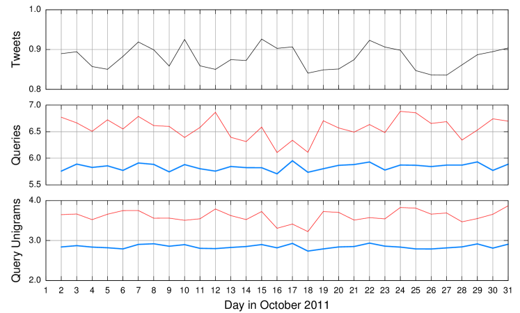
The day-over-day analysis in terms of KL divergence is shown in Figure 1. The figure is broken into three graphs: results over tweets (top), queries (middle), and query unigrams (bottom). The difference between the last two is worth explaining: for analysis in terms of queries, we consider the entire query string (which might consist of multiple terms) as a distinct event. This would, for example, consider “steve jobs” and “jobs” distinct events. For analysis in terms of query unigrams, all queries are tokenized into individual terms, and we consider the multinomial distribution over the term space. Both analyses are useful: when building a query model, for example (?), or extracting query-level features for learning to rank, estimates over the event space of queries would yield more signal, although due to sparsity, one would typically need to back off to unigram statistics. For both the middle and bottom graphs in Figure 1, we further break down analysis in terms of all queries (thin red line) and with trends discarded (thick blue line). We make a few observations: First, there does not appear to be cyclic patterns in day-over-day churn (e.g., day of week effects). Second, eliminating trend queries reduces KL divergence, i.e., successive distributions appear more “similar”—this makes complete sense given the nature of trending topics.

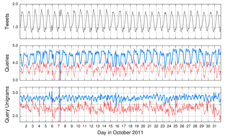
The hour-over-hour analysis in term of KL divergence is shown in Figure 2: this graph is organized in exactly the same way as Figure 1. For tweets and queries, but not query unigrams, we observe strong daily cyclic affects. This is driven by a combination of the rhythm of users’ daily activities and the international nature of Twitter: for example, as users in the United States go to bed and users in Japan wake up, the composition of tweets and queries naturally changes, resulting in churn. Interestingly, we observe that removing trends actually increases churn, i.e., we observe higher KL divergence values. This suggests that the typical lifespan of a trending topic is longer than an hour, i.e., trending topics churn “naturally” at a rate that is slower than hourly, such that removing those events from the distribution increases overall churn. The time that a particular topic trends is a function of many factors: for news, factors include significance of the news event and interactions with competing stories; for internet memes, the lifespan of a particular hashtag is often idiosyncratic. Although not in the Twitter context, see (?) for a quantitative analysis of this “news cycle”.

Table 1 presents churn rates and OOV rates at rank $r=\{10,100,1000,10000\}$ for the day-over-day analysis, averaged across the entire month, for all five experimental conditions: tweets, queries, and query unigrams ($\pm$ trends for the last two). Table 2 shows similar results for the hour-over-hour analysis.

From the search perspective, the OOV rates are interesting, in that they highlight a challenge that real-time search engines must contend with. Take, for example, the day-over-day query unigram OOV rate at rank 1000: results tell us that 7.32% of query terms were not observed in the previous day. This means that for a non-trivial fraction of query unigrams, we have no query-level features: query frequency, clickthrough data to learn from, etc. This is the result at rank 1000, which represents queries pretty close to the head of the distribution. Of course, this particular analysis includes trends (and removing trends reduces the OOV rate substantially), but trend queries remain an important class of queries for which we would like to return high quality results.

Figure 3: KL divergence with respect to first day of October of tweets (top), queries (middle), and query unigrams (bottom). Middle and bottom graphs include analysis without trends (thick blue line) and with trends (thin red line).

Figure 4: KL divergence with respect to first hour in October of tweets (top), queries (middle), and query unigrams (bottom). Middle and bottom graphs include analysis without trends (thick blue line) and with trends (thin red line).

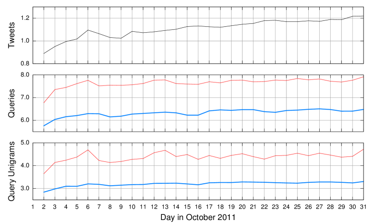
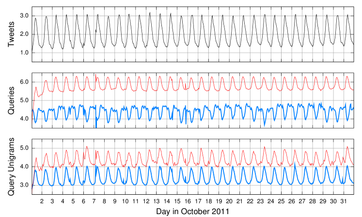
In addition to the interval-over-interval analysis, we repeated the same exact set of experiments with respect to a fixed reference. Figure 3 shows KL divergence of every day in October with respect to the first day. Figure 4 shows KL divergence of every hour in October with respect to the first hour. In the daily condition, we observe weak cyclic effects (i.e., day of week cycles). In Figure 3, for most of the plots we observe a “trough” approximately a week after the initial day. In the hourly condition, we observe strong cyclic affects, as we would expect.

Zooming In

In the context of term churn, rapidly-unfolding events such as natural disasters or political unrest are of particular interest. In such scenarios term frequencies may change significantly over short periods of time as the discussion evolves. Our next analysis examines one such event, the death of Steve Jobs, the co-founder and CEO of Apple, in the afternoon hours of October 5th (around midnight UTC).

Figure 5 shows the KL divergence at 5-minute intervals over a period of 12 hours surrounding the event (thick blue line), contrasting it with the 5-minute KL divergence values over the same hours in the previous day (thin red line). Note the sharp drop in divergence as the real-time query stream focuses on the event. A few hours later, divergence converges to a pattern close to the previous day, although actual values are around 10% less, as significant portions of the query stream continue to discuss the event.

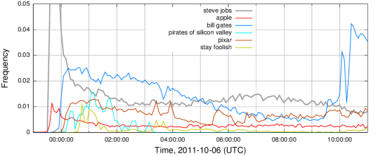
However, even within a particular event, churn of individual queries and terms vary. Figure 6 shows the frequency of several queries related to the event over the same time period, in 5-minute intervals. Note that the patterns do not necessarily correlate in timespan or shape, displaying a range of exponential, linear, and irregular decays over time. One possible conclusion from this data is that a simple approach to account for changes in term frequency over time, such as applying a decay function over the frequency, may not be sufficient. Additionally, it is clear that, at least during major events, sub-hour updates to various collection and query term statistics are essential.

Figure 5: KL divergence of the query stream, in intervals of 5 minutes, over a 12 hour period during a major event (in blue, thick line); the overlay (red, thin) shows the 5-minute KL divergence during the same hours in the preceding day, for reference.

Figure 6: Frequencies of queries related to Steve Jobs’ death over a 12 hour period in 5-minute intervals, normalized to the total number of queries in the interval. At its peak, the query “steve jobs” reaches 0.15 (15% of the query stream); for readability of the other query frequencies, the scale is not stretched to include this point.

	Tweets		Queries
Date	Term	Frequency Ratio	Term	Frequency Ratio
2011-10-03	sunday	3.61	knox	3.45
2011-10-04	weekend	1.62	iphone	4.66
2011-10-05	iphone	1.48	iphone	1.62
2011-10-06	steve	8.28	#stevejobs	7.84
2011-10-09	sunday	3.46	barlow	2.82
2011-10-13	blackberry	3.57	guetta	8.77

Table 3: A sample of top churning terms in tweets (left) and the query stream (right). For each term, the date it was a top term is shown (UTC), as well as the ratio between its frequency on a that day and on the following one.

Churning Terms

Finally, we briefly examine the terms that cause high churn rates in tweets and in the query stream. Table 3 shows unigrams taken from the set of terms that were among the top 500 terms in tweets and queries on one day, and not in the top 2000 terms in the following day; for each day sampled, we show the top non-stopword term.

One interesting observation from an anecdotal examination of the data is that term churn in tweets appears more cyclic and predictable than that in the query stream. While churn levels are high in both, in the case of the query stream this is largely driven by news events, whereas in tweets this is driven by a combination of shifting cyclical interests (e.g., weekends) and news. This suggests that while both tweets and queries experience large amounts of churn, they are qualitatively different. For example, terms like “weekend” and “party” in tweets have frequencies that rise and fall predictably, whereas variations in query frequencies appear to be far less predictable.

Related Work

In the domain of temporal information retrieval, a large body of work on timestamped corpora was driven by TDT—the Topic Detection and Tracking initiative (?). Among the findings relevant to our work is the demonstration that document retrieval benefits from incorporating temporal aspects of the collection into the ranking, e.g., via a language model (?) or by utilizing additional statistics about term frequencies over time, rather than just a global weight (?). Retrieval can also be improved by taking into account the temporal distribution of results and modeling the “burstiness” of events (?).

A body of recent work focuses on the temporal dynamics of Twitter content (rather than search queries). For example, Petrović et al. (?) apply a TDT task—first story detection—to Twitter data, while Wu et al. (?) develop predictors for term churn in tweets.

In the context of web search, Beitzel et al. (?) track the relative popularity of queries throughout the day, as well as the hourly overlap between queries. While exact figures vary by query category, they observe relatively high correlations between the queries of a given hour and the hour following it, with few exceptions related to breaking news. A later study by Kulkarni et al. (?) groups queries by the shape of their popularity over time, showing significant differences over time. However, they focus on a small set of manually-selected queries rather than examining properties of the full query stream.

Of particular interest to us is the work of Teevan et al. (?), who analyze several aspects of Twitter queries and compare them to the web query stream. Interestingly, they observe a lower churn rate on Twitter than on the web. This is counter-intuitive, and may be attributed to the relatively limited amount of data analyzed (our collection is several orders of magnitude larger, as well as annotated for the presence of trends, cleaned of spam, and so on).

Also related to our study is the extensive analysis of modifications to web documents over time, presented in (?). The types of change patterns we observe appear very different from the patterns the authors identify on web pages (e.g., “hockey stick” curves), which naturally makes sense given the context.

Conclusions

This paper examines changes to term distributions on Twitter over time, focusing on the query stream and the implications for ranking in a real-time search system. Our observations can be summarized as follows:

• Churn. Term distributions change rapidly—significantly faster than in web search for the head of the distribution. Even after discounting trending terms promoted by the platform, churn rates of top real-time queries are up to four times higher than those of web searches. For the tail of the distribution, churn drops quickly, and appears to be lower than that observed in web queries.

• Unobserved terms. Similarly, rates of out-of-vocabulary words are higher for top Twitter queries, but lower at the tail of the distribution. This translates to rapid changes in the top user interests, but relative stability in the topics for which users seek real-time results.

• Update frequency. Although query churn is consistently high, during major events it can further increase dramatically, as queries change minute by minute. In fact, to maintain accurate collection statistics requires frequent term count updates—in intervals of 5 minutes or less, according to our data.

• Churn patterns. The time period in which a query remains a top one varies, as does its decay pattern; naïve approaches such as fixed term frequency decays may not be able to correctly model frequency changes over time.

• Predictability. Anecdotal evidence suggests that some query churn may be predicted from past observations, providing a potential source for addressing this issue.

The growing importance of real-time search brings with it several information retrieval challenges; this paper frames one such challenge, that of rapid changes to term distributions, particularly for queries. In follow-up work we plan to evaluate techniques for handling the volatility of the real-time search stream and the limited collection statistics that exist for new queries.

References

- [Adar et al. 2009] Adar, E.; Teevan, J.; Dumais, S.; and Elsas, J. 2009. The web changes everything: understanding the dynamics of web content. WSDM.
- [Allan 2002] Allan, J., ed. 2002. Topic detection and tracking: event-based information organization. Kluwer.
- [Beitzel et al. 2004] Beitzel, S.; Jensen, E.; Chowdhury, A.; Grossman, D.; and Frieder, O. 2004. Hourly analysis of a very large topically categorized web query log. SIGIR.
- [Efron 2010] Efron, M. 2010. Linear time series models for term weighting in information retrieval. JASIST 61:1299–1312.
- [Jones and Diaz 2007] Jones, R., and Diaz, F. 2007. Temporal profiles of queries. TOIS.
- [Kulkarni et al. 2011] Kulkarni, A.; Teevan, J.; Svore, K.; and Dumais, S. 2011. Understanding temporal query dynamics. WSDM.
- [Leskovec, Backstrom, and Kleinberg 2009] Leskovec, J.; Backstrom, L.; and Kleinberg, J. 2009. Meme-tracking and the dynamics of the news cycle. KDD.
- [Li and Croft 2003] Li, X., and Croft, W. 2003. Time-based language models. CIKM.
- [Li 2011] Li, H. 2011. Learning to Rank for Information Retrieval and Natural Language Processing. Morgan & Claypool.
- [Lin, Ryaboy, and Weil 2011] Lin, J.; Ryaboy, D.; and Weil, K. 2011. Full-text indexing for optimizing selection operations in large-scale data analytics. MAPREDUCE Workshop.
- [Olston et al. 2008] Olston, C.; Reed, B.; Srivastava, U.; Kumar, R.; and Tomkins, A. 2008. Pig Latin: A not-so-foreign language for data processing. SIGMOD.
- [Pass, Chowdhury, and Torgeson 2006] Pass, G.; Chowdhury, A.; and Torgeson, C. 2006. A picture of search. InfoScale.
- [Petrović, Osborne, and Lavrenko 2010] Petrović, S.; Osborne, M.; and Lavrenko, V. 2010. Streaming first story detection with application to Twitter. HLT.
- [Ponte and Croft 1998] Ponte, J., and Croft, W. 1998. A language modeling approach to information retrieval. SIGIR.
- [Robertson et al. 1994] Robertson, S. E.; Walker, S.; Jones, S.; Hancock-Beaulieu, M.; and Gatford, M. 1994. Okapi at TREC-3. TREC.
- [Teevan, Ramage, and Morris 2011] Teevan, J.; Ramage, D.; and Morris, M. R. 2011. #TwitterSearch: a comparison of microblog search and web search. WSDM.
- [Wu et al. 2011] Wu, S.; Tan, C.; Kleinberg, J.; and Macy, M. 2011. Does bad news go away faster? ICWSM.
- [Zhai and Lafferty 2002] Zhai, C., and Lafferty, J. 2002. Two-stage language models for information retrieval. SIGIR.