Abstract

The presence of new matter fields charged under the Standard Model gauge group at intermediate scales below the Grand Unification scale modifies the renormalization group evolution of the gauge couplings. This can in turn significantly change the running of the Minimal Supersymmetric Standard Model parameters, in particular the gaugino and the scalar masses. In the absence of new large Yukawa couplings we can parameterise all the intermediate scale models in terms of only two parameters controlling the size of the unified gauge coupling. As a consequence of the modified running, the low energy spectrum can be strongly affected with interesting phenomenological consequences. In particular, we show that scalar over gaugino mass ratios tend to increase and the regions of the parameter space with neutralino Dark Matter compatible with cosmological observations get drastically modified. Moreover, we discuss some observables that can be used to test the intermediate scale physics at the LHC in a wide class of models.

1 Introduction

The apparent unification of the Standard Model (SM) gauge couplings can be regarded as a major achievement of the Minimal Supersymmetric Standard Model (MSSM). Indeed, gauge couplings unification represents the most convincing hint of a Grand Unified Theory (GUT) at very high energy scales. Typically, unification is achieved by assuming the absence of new physics between the electroweak (EW) (or supersymmetric (SUSY)) scale and the GUT scale, $M_{\rm GUT}\approx 10^{16}$ GeV. In fact, the presence of fields charged under the SM gauge group at intermediate scales below $M_{\rm GUT}$ modifies the renormalization group (RG) evolution of the gauge couplings and in general spoils the successful gauge coupling unification. On the other hand, the presence of “oases” of new physics in the “big desert” between 1 TeV and $M_{\rm GUT}$ is a natural prediction of many extensions of the MSSM. For instance, neutrino masses point towards a lepton number breaking scale some orders of magnitude below $M_{\rm GUT}$. The fields associated with such new scale can be charged under the SM gauge group, as in the case of the so-called type-II [1] or type-III [2, 3] seesaw models. Also, the dynamical generation of the SM flavour hierarchy typically requires heavy vectorlike quarks or Higgs fields as mediators of the flavour symmetry breaking [4] (for a recent discussion see [5]). Finally, intermediate scales are present in models where the breaking of the GUT symmetry to the SM one is achieved via intermediate steps, such as Pati-Salam models [6] or left-right symmetric models [7].

Gauge coupling unification can be maintained by appropriately choosing the masses of the new fields or by embedding them in particular sets (the simplest ones being complete multiplets of a GUT group, but more general choices are also possible [8]). Nevertheless, the value of the unified coupling is modified by the presence of the new fields. This can in turn significantly change the RG running of the MSSM parameters, in particular the gaugino and the scalar masses (if the SUSY breaking occurs at scales higher than the intermediate scale). Therefore, one can expect a potentially observable impact of the intermediate-scale physics on the low-energy SUSY spectrum and phenomenology. Recently, the possible consequences of intermediate scales have been discussed in a variety of specific models [9]-[15].

In this work we are going to discuss the phenomenological consequences of the intermediate scale, due to the modified running of the MSSM parameters. We assume that the SUSY breaking scale is equal or larger than $M_{\rm GUT}$, such that the running of the SUSY breaking masses is indeed affected by the presence of the intermediate scale. Without restricting to a specific model, we consider generic sets of new matter fields (i.e. chiral superfields) in vectorlike representations of the SM gauge group, forming approximately degenerate multiplets of a GUT group. This allows us to highlight the common features and the possible observable consequences of this kind of models, as it ensures that gauge coupling unification is maintained independently of the intermediate scale and $M_{\rm GUT}$ is the same as in the ordinary MSSM. These properties are in general not satisfied in the case of multiple step breaking of the GUT symmetry to the SM, i.e. in the presence of new gauge bosons (vector superfields) below $M_{\rm GUT}$ (see however [8]). Therefore, we assume the gauge group to be $SU(3)\times SU(2)\times U(1)$ up to the GUT scale. However, as we will see, the effects we are going to discuss mainly depends on the fact that, in the presence of new matter, the SM gauge couplings unify at a common value that is larger than in the “big desert” scenario. As a consequence, we expect that our findings qualitatively occur in broader classes of models, whenever the latter feature is realised.

The rest of the paper is organised as follows: in section 2 we discuss the main effect, i.e. the modification of the running of the MSSM parameters in the presence of new fields at intermediate scales. In section 3 we discuss a few observables that can be used to test the intermediate scale at the LHC, while in sections 4 and 5 we analyse the consequences for the neutralino relic density and the proton decay, respectively. Finally, in section 6 we conclude. Details on analytical solutions of the one loop running and a discussion on the impact of two loop RGEs are given in the two appendices.

2 MSSM running with an intermediate scale

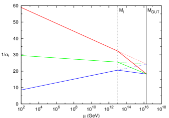
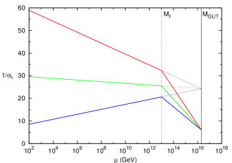
Figure 1: Modification of the gauge couplings running in the presence of matter at the intermediate scale $M_{I}=10^{13}$ GeV. In the left panel we take $\Delta b=5$ (corresponding e.g. to a single $\bf 24$ representation of $SU(5)$), in the right panel we take $\Delta b=15$ (e.g. $3\times{\bf 24}$).

Our starting assumption is the presence of a set of chiral superfields in complete vectorlike representations of SU(5) at an intermediate scale $M_{I}<M_{\rm GUT}$. This choice does not spoil the successful, one loop, gauge coupling unification of the MSSM, as the running of the three couplings gets deflected in the same way. In other words, the successful prediction for $\alpha_{3}(M_{Z})$ (and $M_{\rm GUT}$) is not modified. However, it is well known that the fields at $M_{I}$ make the running above this scale “stronger” and the gauge couplings finally unify at a value $\alpha_{U}$ larger than in the MSSM. This effect can be seen by solving the one loop RGEs:

$$\frac{1}{\alpha_{U}}=\frac{1}{\alpha_{i}(M_{Z})}-\frac{b^{SM}_{i}}{2\pi}\ln\frac{M_{S}}{M_{Z}}-\frac{b^{0}_{i}}{2\pi}\ln\frac{M_{\rm GUT}}{M_{S}}-\frac{\Delta b}{2\pi}\ln\frac{M_{\rm GUT}}{M_{I}}\equiv\frac{1}{\alpha^{0}_{U}}-\frac{\Delta b}{2\pi}\ln\frac{M_{\rm GUT}}{M_{I}}\,,$$ (1)

where $\alpha^{0}_{U}$ is the unified coupling in the MSSM without intermediate scale ($\alpha^{0}_{U}\simeq 1/25$), $b_{i}^{SM}=(41/10,-19/6,-7)$ and $b^{0}_{i}=(33/5,1,-3)$ are respectively the SM and MSSM $\beta$-function coefficients for $\alpha_{i}$ ($i=1,2,3$), $\Delta b$ is the universal contribution of the additional fields at $M_{I}$ and $M_{S}$ is the typical low-energy SUSY scale. $\Delta b$ is given by the sum of the Dynkin indexes of the SU(5) representations of the fields at $M_{I}$. From Eq. (1), we see that, since $\Delta b\geq 0$ for chiral superfields, the unified coupling $\alpha_{U}$ is in general larger than the MSSM one, $\alpha_{U}\geq\alpha^{0}_{U}$. This effect is exemplified in Fig. 1, for $M_{I}=10^{13}$ GeV and $\Delta b=5,~{}15$. The dashed lines represent the ordinary MSSM running.

Clearly, for a given $\Delta b$, Eq. (1) will give a lower bound on the scale $M_{I}$ by requiring perturbativity of the gauge couplings up to the GUT scale. We can see the perturbativity bound in Fig. 2, where contours for $1/\alpha_{U}$ are plotted on the $M_{I}$-$\Delta b$ plane. The white area in the plot is excluded since it corresponds to $1/\alpha_{U}<0$, i.e. to a Landau pole below the GUT scale. Looking at the left panel, where results obtained using Eq. (1) are shown, we see for instance that with $\Delta b=15$ (e.g. corresponding to $3\times{\bf 24}$), the intermediate scale is constrained to be $M_{I}\gtrsim 10^{12}$ GeV, while in case of the type-II seesaw ($\Delta b=7$) we have $M_{I}\gtrsim 10^{7}$ GeV. On the other hand, it is remarkable that $M_{I}$ can be as low as the TeV scale, provided that $\Delta b\lesssim 5$.

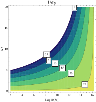
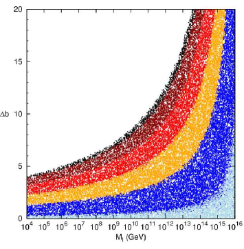
Figure 2: Contours on the plane $M_{I}$-$\Delta b$ of the inverse of the unified gauge coupling $1/\alpha_{U}$ (considering one loop RGEs in the left panel, two loops in the right one). The white region is excluded from the requirement of perturbativity of the couplings up to the GUT scale. In the right panel light blue corresponds to $1/\alpha_{U}>25$, blue to $>20$, yellow to $>15$, red to $>10$, brown to $>5$ and black to $>0$. We refer to Appendix B for details on the meaning of $\Delta b$ in the two loop case.

We thus observe that already with this simple requirement, we can exclude a large part of the parameter space.

The figure in the left panel was derived using Eq. (1) but does not qualitatively change considering two loops RGEs, as can be seen in the right panel of Fig. 2. Notice, in particular, that the region far from the Landau pole is practically unaltered, while large modifications appear for $\alpha_{U}\gtrsim 0.2$. It is evident from this plot that constraints derived at one loop are then conservative. Details on two loops RGEs will be given in Appendix B.

As we will see in the following, the main effects we are going to discuss are linked to the larger values of $\alpha_{U}$ induced by the intermediate scale physics and therefore can be conveniently illustrated in terms of two additional parameters only, $M_{I}$ and $\Delta b$.

2.1 Running of gaugino masses

Let us now move to consider the effect of intermediate-scale physics on the gaugino mass running. As we know, the $\beta$-functions of the gaugino masses are related to those of the corresponding gauge coupling, hence the modification of the running of the gauge couplings above $M_{I}$ will affect the running of the gaugino mass parameters, $M_{i}$ ($i=1,2,3$), as well. This effect can be easily related to the increase of the unified gauge coupling $\alpha_{U}$. We can see this from the usual one loop relation among gaugino masses and gauge couplings, which is not modified in our scenario:

$$M_{i}(\mu)=M_{i}(M_{\rm GUT})\,\frac{\alpha_{i}(\mu)}{\alpha_{U}}\,,$$ (2)

where $\mu$ is the renormalization scale. Obviously, the low-energy gaugino mass ratios ($M_{1}:M_{2}:M_{3}\approx 1:2:6$ in the case of gaugino mass unification) are then not modified by the presence of the intermediate scale. However, for given initial values $M_{i}(M_{\rm GUT})$, the low-energy gaugino masses result smaller than in the MSSM, since $\alpha_{U}$ is larger. This effect is depicted in Fig. 3 for the same choices of $M_{I}$ and $\Delta b$ of Fig. 1, assuming gaugino mass unification with $M_{i}(M_{\rm GUT})=M_{1/2}$.

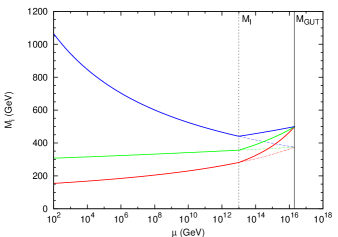
Figure 3: Running of gaugino masses for $\Delta b=5$ (left), $\Delta b=15$ (right). Solid lines correspond to the running with new matter at the intermediate scale $M_{I}=10^{13}$ GeV, while dashed lines represent the ordinary MSSM running, corresponding to the same values for $M_{i}$ at low energy.

Above the scale $M_{I}$, gaugino masses can have a very strong running, while below the usual MSSM evolution is clearly recovered. The dashed lines in the plots represent the ordinary MSSM running, giving the same gaugino mass spectrum at low energy. It is clear from Eq. (2) that, in order to obtain the same gaugino masses at low energy, the starting unified mass $M^{0}_{1/2}$ in absence of the intermediate scale must be smaller than $M_{1/2}$:

$$M^{0}_{1/2}=M_{1/2}\,\frac{\alpha_{U}^{0}}{\alpha_{U}}=M_{1/2}\left(1-\alpha_{U}^{0}\frac{\Delta b}{2\pi}\ln\frac{M_{\rm GUT}}{M_{I}}\right)\,.$$ (3)

At this stage, this might be seen as a trivial rescaling of $M_{1/2}$, i.e. a larger value at $M_{\rm GUT}$ than in the MSSM is required to reproduce a given gaugino spectrum in the presence of the intermediate scale. However, this affects non-trivially the running of other MSSM parameters, in particular scalar masses, as we are going to discuss in the following.

2.2 Running of scalar masses

In order to see the effect on the evolution of the scalar masses, let us recall the form of the one loop RGEs for the soft SUSY breaking mass terms. Denoting sfermion and Higgs fields as $\phi$, we schematically have:

$$\frac{d}{dt}m^{2}_{\phi}=-\frac{2}{\pi}\sum_{i}C_{i}(r_{\phi})\alpha_{i}(t)|M_{i}(t)|^{2}+\frac{1}{16\pi^{2}}(Y^{2}m^{2}_{\phi^{\prime}}+A^{2})\,,$$ (4)

where we can choose $t=\ln(\mu/M_{\rm GUT})$ and $C_{i}(r_{\phi})$ is the quadratic Casimir of the representation $r_{\phi}$ of the field $\phi$. $Y^{2}$ generically denotes Yukawa couplings (with $m^{2}_{\phi^{\prime}}$ we indicate that soft masses of different scalars can appear) and similarly $A^{2}$ schematically refers to contributions proportional to the A-terms. From Eq. (4), we can see the well known behaviour in the scalar masses evolution: in the running from $M_{\rm GUT}$ to low energies the gauge part of the $\beta$-function ($\propto\alpha_{i}(t)|M_{i}(t)|^{2}$) tends to increase the scalar mass $m^{2}_{\phi}$, while the terms proportional to the Yukawa and the trilinear couplings have the opposite effect and tend to decrease it. This latter effect can be however sizeable only if large third generation Yukawas and A-terms are involved (such as in the case of the stop and $H_{u}$ masses, where these terms are proportional to $y_{t}^{2}$). Therefore for what concerns 1st and 2nd generation sfermion masses, we can consider only the gauge term in the $\beta$-functions and obtain simple analytical solutions of the one loop RGEs (see Appendix A).

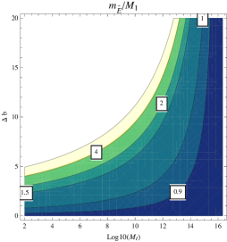
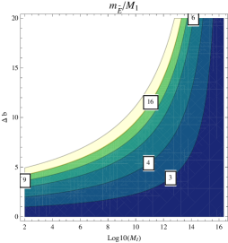
Figure 4: Ratio of the 1st or 2nd generation RH sleptons over the bino mass $M_{1}$ for $m_{\tilde{E}}/M_{1}=0,\,1,\,2$ at $M_{\rm GUT}$.

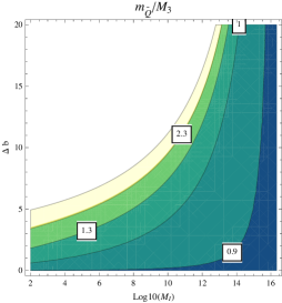
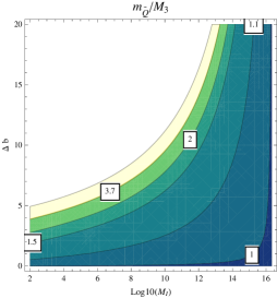
Figure 5: Ratio of the 1st or 2nd generation LH squarks over the gluino mass $M_{3}$ for $m_{\tilde{Q}}/M_{3}=0,\,1,\,2$ at $M_{\rm GUT}$.

How is the running of scalar masses affected by the intermediate scale fields? As we have seen in Figs. 1 and 3, $\alpha_{i}$ and $M_{i}$ run to larger values above $M_{I}$. Starting with the same scalar and gaugino masses at $M_{\rm GUT}$ and running down to the EW scale, in the presence of the intermediate scales, scalar masses will grow less than in the MSSM case, because of the fast decrease of gaugino masses shown in Fig. 3. But while considering only gaugino masses the MSSM spectrum could be recovered just by rescaling the GUT values $M_{i}(M_{\rm GUT})$, this is not any longer true if scalars are also taken into account. In other words, the intermediate scale has low-energy consequences in form of a distortion of the SUSY spectrum. In fact, for the same values of low-energy gaugino masses as in the MSSM, scalar masses feel an enhancement of the gauge part of the $\beta$-function in Eq. (4) in the first stage of the running, between $M_{\rm GUT}$ and $M_{I}$, due to larger couplings and heavier gauginos at high energy. This means that the scalar masses run to larger values, or, more precisely, the presence of intermediate-scale fields tends to increase the scalar over gaugino mass ratios, $m_{\phi}/M_{i}$. Notice that here, in order to restrict our analysis to model independent effects, we are assuming no large (i.e. $\mathcal{O}(1)$) Yukawa couplings among the MSSM fields and the new matter. In that case the scalar masses would receive a further negative contribution, as shown in Eq. 4. Such an assumption is also motivated by the protection from new large flavour violating effects: for instance in type II or III seesaw models the new Yukawas are typically constrained to values that have a negligible impact on the SUSY spectrum ($\lesssim(0.1)$) by the bounds on lepton flavour violating processes [10, 11, 16].

The effect sketched above can be seen by looking at the RGE of such mass ratios. In particular, let us consider the ratio of the right-handed (RH) selectron and Bino masses, ${m^{2}_{\tilde{E}}}/{M_{1}^{2}}$:

$$\frac{d}{dt}\left(\frac{m^{2}_{\tilde{E}}}{M_{1}^{2}}\right)=-\frac{6}{5\pi}\alpha_{1}-\left(\frac{m^{2}_{\tilde{E}}}{M_{1}^{2}}\right)\frac{b_{1}}{\pi}\alpha_{1}\,.$$ (5)

Given the minus sign in the $\beta$-function, the ratio increases in the running from high to low scale and, in the presence of intermediate scale physics, it increases more, due to a larger gauge coupling in the high-energy part of the running. This can be also shown by means of the one loop formulae of the Appendix A. From Eqs. (28, A), we get:

$$\frac{m^{2}_{\tilde{E}}}{M_{1}^{2}}(M_{S})= \frac{m^{2}_{\tilde{E}}(M_{\rm GUT})}{M_{1}^{2}(M_{S})}+\frac{6}{5b^{0}_{1}}\left[\frac{b^{0}_{1}}{b^{0}_{1}+\Delta b}\frac{\alpha_{U}^{2}}{\alpha_{1}^{2}(M_{S})}+\frac{\Delta b}{b^{0}_{1}+\Delta b}\frac{\alpha_{1}^{2}(M_{I})}{\alpha_{1}^{2}(M_{S})}-1\right]\,.$$ (6)

For a given low-energy value for $M_{1}(M_{S})$ and a given high-energy starting value $m_{\tilde{E}}(M_{\rm GUT})$, the ratio above tends to grow in the presence of the intermediate scale (i.e. increasing $\Delta b$ and/or decreasing $M_{I}$), since ${\alpha_{U}^{2}}/{\alpha_{1}^{2}(M_{S})}$ strongly grows, according to Eq. (1).

The effect exemplified above is general for all scalar masses. This is the main point of our discussion and it is represented in Figs. 4-5, where the low-energy ratios of the 1st or 2nd generation RH sleptons, $m_{\tilde{E}}$, over the Bino mass $M_{1}$ and the 1st or 2nd generation left-handed (LH) squarks, $m_{\tilde{Q}}$, over the gluino mass $M_{3}$ are plotted for different GUT values of, respectively, $m_{\tilde{E}}/M_{1}$ and $m_{\tilde{Q}}/M_{3}$. Again, we made use of the analytical formulae given in the Appendix A. As in Fig. 1, the white area corresponds to a Landau pole occurring below the GUT scale. The fact that low-energy mass ratios increase by introducing new matter at the intermediate scale (i.e. with increasing $\alpha_{U}$) leads to potentially observable consequences at the LHC and affects DM phenomenology, as we will discuss in the following sections.

2.3 Higgs soft masses and EWSB

Apart from scalar and gaugino masses, the presence of intermediate scale clearly affects the running of the Higgs mass parameters $m^{2}_{H_{u}}$ and $m^{2}_{H_{d}}$ too, and thus affects the EWSB and the higgsino mass $\mu$. Once correct EWSB is imposed, $\mu$ is given (at tree level) by the well-known expression:

$$|\mu|^{2}=-m^{2}_{H_{u}}-\frac{M_{Z}^{2}}{2}+\mathcal{O}(m^{2}_{H_{u,d}}/(\tan\beta)^{2})\,.$$ (7)

The higgsino mass $\mu$ enters the neutralino mass matrix and it is thus crucial to determine the composition of the lightest neutralino and whether it can be a good dark matter (DM) candidate.

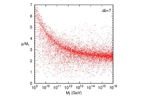
Figure 6: Ratio $\mu/M_{1}$ vs. $M_{I}$ for a numerical scan of the parameter space with $\Delta b$=7.

In the usual MSSM $m_{H_{u}}$ runs to negative values at low energy due to the terms in the $\beta-$function proportional to $y_{t}^{2}$, the top Yukawa coupling. In spite of the fact that $y_{t}$ at high energy is somewhat smaller when an intermediate scale is present, the increase of the scalar over gaugino mass ratio turns out to be the dominant effect. Since stop masses enter the terms $\propto y_{t}^{2}$ in the RGEs, the net effect is that the ratio $m_{H_{u}}/M_{i}$ tends to run to even more negative values when new physics at intermediate scale is present and thus $\mu/M_{i}$ gets increased (cf. Eq. (7)). This effect in shown Fig. 6 for the illustrative case of $\Delta b$=7 and universal boundary conditions at the GUT scale.

The clear tendency shown in the figure generically tells us that: (i) intermediate scale models tend to worsen the fine-tuning problem of the MSSM, (ii) the lightest neutralino $\tilde{\chi}_{1}^{0}$ tends to be more and more $\tilde{B}$-like. However, independently of how strong is the effect of the intermediate scale, this does not rule out configurations in the parameter space that give $\mu\approx M_{1}$, i.e. with low fine-tuning and a neutralino relic density in agreement with WMAP observations, due to the sizable higgsino component of $\tilde{\chi}_{1}^{0}$ [19]. Furthermore, non-universal Higgs boundary conditions at the high scale can affect this result.

3 LHC observables

As we discussed above, intermediate scale physics can leave a clear imprint on the low-energy SUSY spectrum. The question is whether this can be observed at the LHC. In order to isolate the effect of the intermediate scale, we need observables that are as much independent as possible of high-scale scalar and gaugino masses. For instance, even if the low-energy scalar over gaugino mass ratios grow in the presence of intermediate scale fields, as shown in Figs. 4 and 5, there is also a strong dependence on the high-energy initial conditions, hence it seems hard to disentangle the two effects. However, even at this stage, we can see that SUSY searches at the LHC can be affected by the intermediate scale. Let us consider, for instance, the first panel of Fig. 5, that corresponds to the case of vanishing squark masses at the GUT scale. If we do not allow $m^{2}_{\tilde{Q}}(M_{\rm GUT})<0$, such configuration clearly gives the least possible ratio $(m_{\tilde{Q}}/M_{3})^{\rm min}$ at low energy . While in the ordinary MSSM $(m_{\tilde{Q}}/M_{3})^{\rm min}\approx 1$, we see that the intermediate scale can easily push the minimum ratio to values larger than 2. This means that the configuration $M_{\tilde{g}}\approx m_{\tilde{Q}}$ that gives the highest sensitivity in the LHC SUSY searches (see e.g. [20]) would not be theoretically accessible and, independently of the starting values for the soft masses at high energy, only the case $M_{\tilde{g}}<m_{\tilde{Q}}$ (or even $M_{\tilde{g}}\ll m_{\tilde{Q}}$) would be possible. On the other hand, observing the case $M_{\tilde{g}}\approx m_{\tilde{Q}}$ at the LHC would give an upper bound to $\alpha_{U}$ and thus strongly constrain the $\Delta b$ and $M_{I}$ parameters.

In the following we will describe other quantities that are to large extent model-independent and can be used to constrain the presence of new physics at intermediate scales.

3.1 Mass Invariants

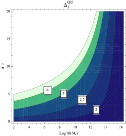
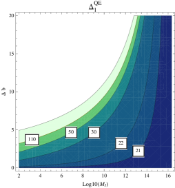
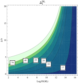
Figure 7: Contours for the mass invariants $\Delta^{QU}_{1}$, $\Delta^{QE}_{1}$, $\Delta^{DL}_{1}$, defined in Eq. (11), for M${}_{S}=1$ TeV.

If we assume gaugino mass unification, the gaugino and first generations sfermion masses can be written (at one loop) in the form:

$$M_{i}(M_{S}) = A_{i}(M_{S},\Delta b,M_{I})\,M_{1/2}$$ (8)

$$m^{2}_{\tilde{f}}(M_{S}) = m_{\tilde{f}}^{2}(M_{\rm GUT})+B_{\tilde{f}}(M_{S},\Delta b,M_{I})\,M_{1/2}^{2}\,,$$ (9)

where the coefficients $A_{i}$ and $B_{\tilde{f}}$, as functions of $\Delta b$ and $M_{I}$, can be read in Eqs. (26) and (28, A).

It is clear that in the combination

$$\Delta^{ff^{\prime}}_{i}\equiv\frac{m^{2}_{\tilde{f}}-m^{2}_{\tilde{f^{\prime}}}}{M_{i}^{2}}$$ (10)

the explicit dependence on the GUT-scale parameters drops, if $m_{\tilde{f}^{\prime}}^{2}(M_{\rm GUT})=m_{\tilde{f}}^{2}(M_{\rm GUT})\equiv m_{0}^{2}$ as in CMSSM-like scenarios or, more in general, in the case of GUT-symmetric initial conditions (a well-motivated assumption in our setup, as we are requiring unification). Notice, however, that $A_{i}$ and $B_{\tilde{f}}$ do not depend on $\Delta b$ and $M_{I}$ only, but logarithmically on the SUSY mass-scale $M_{S}$ as well. This induces a residual dependence of the parameters $\Delta^{ff^{\prime}}_{i}$ on the initial conditions $m_{0}$ and $M_{1/2}$ that can be relevant, as we are going to show in the following.

In Ref. [9], it has been pointed out that mass invariants of the kind of Eq. (10) are very sensitive to intermediate scale fields and can be thus useful to discriminate among different SUSY seesaw models (see also [12, 13]). Here we want to generalise that result and study these invariants for generic values of $M_{I}$-$\Delta b$. As in Ref. [9], we consider the SU(5)-inspired combinations:

$$\Delta^{QU}_{1}\equiv\frac{m^{2}_{\tilde{Q}}-m^{2}_{\tilde{U}}}{M_{1}^{2}},\quad\quad\Delta^{QE}_{1}\equiv\frac{m^{2}_{\tilde{Q}}-m^{2}_{\tilde{E}}}{M_{1}^{2}},\quad\quad\Delta^{DL}_{1}\equiv\frac{m^{2}_{\tilde{D}}-m^{2}_{\tilde{L}}}{M_{1}^{2}}.$$ (11)

Contours for these quantities on the $M_{I}-\Delta b$ plane are shown in Fig. 7 (taking $M_{S}=1$ TeV). As we can see, the invariants rapidly grow for increasing $\alpha_{U}$. This is a further consequence of the effect described in the previous section: $m^{2}_{\tilde{Q}}/M_{1}^{2}$ increases with $\alpha_{U}$ and does it more than $m^{2}_{\tilde{U}}/M_{1}^{2}$ that does not feel the contribution of SU(2) gauginos, thus $\Delta^{QU}_{1}$ grows too. An analogous effect occurs for the other invariants. Measurements of the SUSY spectrum at the LHC can be then potentially used to derive precise information on the nature of the new physics possibly present at intermediate scales. If the invariants of Eqs. (11) will be measured to differ significantly from the MSSM values ($\Delta^{QU}_{1}\approx 2$, $\Delta^{QE}_{1}\approx 21$, $\Delta^{DL}_{1}\approx 17$ for $M_{S}=1$ TeV), this might be a hint of new physics below the GUT scale (that can provide information on the scale and nature of it), or simply a signal that soft masses are not universal at the GUT scale. In principle, it should be still possible to identify the first case by reconstructing more than one invariant, since the three invariants exhibit robust correlations, as Fig. 7 shows.

As in the case of $\alpha_{U}$, the above effect is strengthened at two loops, especially in the vicinity of the Landau pole. The typical correction is however $\lesssim$ 10% (see Appendix B) and hence the plots of Fig. 7 still give a good estimate of the impact of the intermediate scale on these quantities.

As we mentioned above, the numerical values of the invariants still depend on the SUSY scale. For instance, in the range $M_{Z}\leq M_{S}\leq 3$ TeV, we observe a variation of $\Delta^{ff^{\prime}}_{i}$ up to $60\%$, which of course might spoil any attempt to constrain intermediate scale with them. Even if it is true that once the sparticle masses will be measured, also the SUSY scale can be set, we look for mass invariants which are more independent on the SUSY scale.

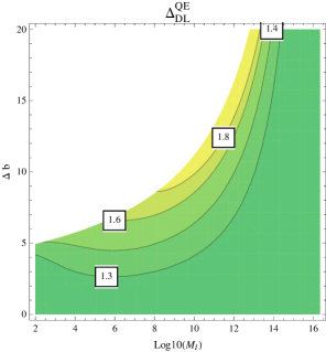
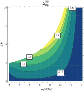
Figure 8: Contours for the mass invariants $\Delta^{QE}_{DL}$, $\Delta^{QU}_{DL}$, defined in Eq. (12), for M${}_{S}=1$ TeV.

We consider ratios of the above invariants, i.e. simply ratios of scalar mass differences:

$$\Delta^{f_{1}f_{2}}_{f_{3}f_{4}}\equiv\frac{m^{2}_{\tilde{f}_{1}}-m^{2}_{\tilde{f}_{2}}}{m^{2}_{\tilde{f}_{3}}-m^{2}_{\tilde{f}_{4}}}\,.$$ (12)

Compared to the quantities in Eq. (11), these ones have a much milder dependence on $M_{S}$. This is true in particular for $\Delta^{QE}_{DL}=(m^{2}_{\tilde{Q}}-m^{2}_{\tilde{E}})/(m^{2}_{\tilde{D}}-m^{2}_{\tilde{L}})$, where the variation in the range $M_{Z}\leq M_{S}\leq 3$ TeV is just of a few percent. Countour plots for these invariants are shown in Fig. 8. Besides using the analytical one loop expressions, we numerically computed the invariants including two loops contributions. The results are shown in Appendix B. The effect of the intermediate scale is again stronger than at one loop and deviates from Fig. 8 quite sizeably close to the Landau pole.

We have shown that mass invariants can in principle give information and strong constraints on $\Delta b$ and $M_{I}$. They might even exclude, if observed to be close to the CMSSM predictions, the presence of fields charged under the SM gauge group at scales below $M_{\rm GUT}$. However, it is difficult to say whether all the SUSY masses entering these invariants can be measured with sufficient precision at the LHC. Clearly this question depends on the actual mass-scale of the SUSY particles, as well as on some features of the spectrum, and is beyond the purposes of the present discussion. Let us only notice that, if the slepton masses can be reconstructed from cascade decays of heavier particles (see the next section), the invariants involving squark and slepton mass differences should not be difficult to obtain, given the typical hierarchy between coloured and uncoloured sfermions. Moreover, Figs. 7 and 8 show that, even in presence of uncertainties as large as 10%, the invariants can provide very useful information on the intermediate scale and discriminate among different scenarios. It might be much more difficult to resolve experimentally squark mass differences like $m^{2}_{\tilde{Q}}-m^{2}_{\tilde{U}}$. However, we notice that intermediate scale physics might help in this sense. In fact, the relative mass-splitting $(m_{\tilde{Q}}-m_{\tilde{U}})/m_{\tilde{Q}}$ (that can at most be $\approx 5$% in the CMSSM) increases with $\alpha_{U}$ too and can reach values larger than 10%.

3.2 Kinematic Edges in Cascade Decays

Let us now investigate whether the distortion of the spectrum can be studied by means of kinematic observables potentially measurable at the LHC experiments. We consider the typical cascade decay depicted in Fig. 9.

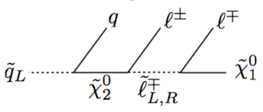
Figure 9: An example of a cascade decay.

The intermediate particles are real if the following condition is fulfilled:

$$m_{\tilde{Q}}>m_{{\tilde{\chi}}^{0}_{2}}>m_{\tilde{\ell}_{L,R}}>m_{{\tilde{\chi}}^{0}_{1}}\,.$$ (13)

Consequently, the invariant-mass distributions of the outgoing SM particles (jets and isolated leptons) exhibit sharp kinematic end-points [21]. Notice that, depending on the spectrum, zero, one or two sharp edges can be present. Indeed, if for example both $m_{\tilde{\ell}_{L}}$ and $m_{\tilde{\ell}_{R}}$ satisfy the above inequality, then two edges could be observed, while only one will be there if only one of the two –typically $m_{\tilde{l}_{R}}$– satisfies it. The position of the end-points of the distributions can be expressed as a function of the SUSY masses:

$$m_{\ell\ell}^{\rm max} = \sqrt{\frac{(m^{2}_{{\tilde{\chi}}^{0}_{2}}-m^{2}_{\tilde{\ell}})(m^{2}_{\tilde{\ell}}-m^{2}_{{\tilde{\chi}}^{0}_{1}})}{m^{2}_{\tilde{\ell}}}}$$ (14)

$$m_{\ell j}^{\rm max} = \sqrt{\frac{(m_{\tilde{q}}^{2}-m^{2}_{{\tilde{\chi}}^{0}_{2}})(m^{2}_{{\tilde{\chi}}^{0}_{2}}-m_{\tilde{\ell}}^{2})}{m^{2}_{{\tilde{\chi}}^{0}_{2}}}}$$ (15)

$$m_{\ell\ell j}^{\rm max} = \sqrt{\frac{(m_{\tilde{q}}^{2}-m^{2}_{{\tilde{\chi}}^{0}_{2}})(m^{2}_{{\tilde{\chi}}^{0}_{2}}-m^{2}_{{\tilde{\chi}}^{0}_{1}})}{m^{2}_{{\tilde{\chi}}^{0}_{2}}}}\,,$$ (16)

and can therefore be used to reconstruct the SUSY spectrum [21]. As any combination of SUSY masses, these observables are also modified in the presence of the intermediate scale.

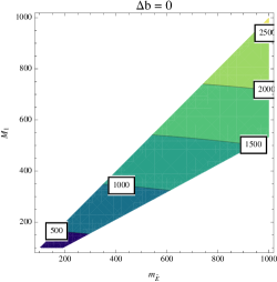
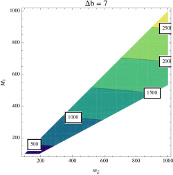
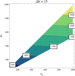
Figure 10: Value of the kinematic edge $m_{\ell\ell j}^{\rm max}$ in the cascade decay of Fig. 9 on the plane $(m_{\tilde{E}},M_{1})$ for $\Delta b=0,7,15$ at $M_{I}=10^{13}$ GeV, respectively.

As an example, in Fig. 10 we plot contours for $m_{\ell\ell j}^{\rm max}$ in the plane of the physical masses $(m_{\tilde{E}},\,M_{1}\approx m_{{\tilde{\chi}}^{0}_{1}})$ for three different choices of $\Delta b$ and a fixed $M_{I}$. As expected, the value of the edge changes with the intermediate scale. Again, if it is possible to independently measure the RH slepton and the neutralino masses (e.g. from $m_{\ell\ell}^{\rm max}$ and $m_{\ell j}^{\rm max}$ together with jets and missing $E_{T}$ distributions) and the edge of $m_{\ell\ell j}$, this could provide a further way to test intermediate scale physics.

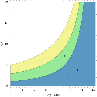
Figure 11: Maximum number of edges in the cascade decay of Fig. 9 on the plane $(M_{I},\Delta b)$.

As we have mentioned above, depending on the spectrum (in particular whether the sleptons are lighter than the second neutralino) the number of edges can vary. Indeed, as we have extensively discussed, the effect of the intermediate scale is precisely that of increasing the ratio of the scalar over gaugino masses and thus making the condition of Eq. (13) more difficult to be satisfied. In order to illustrate this point, we have obtained the maximum number of possible edges in the $m_{\ell\ell}$ and $m_{\ell j}$ invariant mass distributions as a function of $(M_{I},\Delta b)$. This quantity is independent of the details of the spectrum. The result is shown in Fig. 11. As we can see, the effect of the intermediate scale can be such that the cascade decay of Fig. 9 is never kinematically allowed (in other words $m_{\tilde{\ell}_{L,R}}>m_{{\tilde{\chi}}^{0}_{2}}$ always) or just for the lighter sleptons for any choice of sfermion and gaugino masses at high energy. It is then clear that, if for instance two clear edges will be observed in di-electron or di-muon distributions, we will be able to exclude a large portion of the $(M_{I},\Delta b)$ parameter space. On the other hand, if no edges are observed at all, intermediate scale physics would remain unconstrained as it is always possible to choose high-energy initial conditions such that $m_{\tilde{\ell}_{L,R}}>m_{{\tilde{\chi}}^{0}_{2}}$ .

4 Neutralino Dark Matter

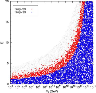
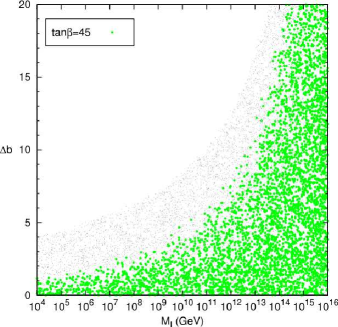
Figure 12: Left: region on the $(M_{I},\Delta b)$ plane where the correct relic density for $\tilde{\chi}^{0}_{1}$ is obtained via $\tilde{\tau}$ coannihilation (blue points corresponds to $\tan\beta=10$, red to $\tan\beta=30$). Right: the same for the A-funnel region. The grey dots in the background mark the region consistent with the perturbativity bounds.

The modification of the SUSY spectrum described in the previous sections can destabilise the regions of the parameter space where precise relations among the parameters are required in order to fulfill the WMAP bound on DM relic abundance.

It is well known that the lightest neutralino of the MSSM, $\tilde{\chi}^{0}_{1}$, typically $\tilde{B}$-like (i.e. $m_{\tilde{\chi}^{0}_{1}}\simeq M_{1}$), is overproduced in the early universe, unless the neutralino (co)annihilation cross-section is enhanced by particular conditions. Such conditions define few regions of the parameter space where the WMAP bound is satisfied: (i) the $\tilde{\tau}$ coannihilation region, where the correct relic density is achieved thanks to an efficient $\tilde{\tau}$-$\tilde{\chi}^{0}_{1}$ coannihilation, which requires $m_{\tilde{\tau}_{1}}\approx m_{\tilde{\chi}^{0}_{1}}$ [22]; (ii) the “focus-point” region, where the Higgsino-component of $\tilde{\chi}^{0}_{1}$ is sizable, i.e. $\mu\approx M_{1}$ [19]; (iii) the A-funnel region, where the neutralino annihilation is enhanced by a resonant s-channel CP-odd Higgs exchange, if $m_{A}\simeq 2\times m_{\tilde{\chi}^{0}_{1}}$ [23].

Let us consider first the $\tilde{\tau}$ coannihilation region. In the CMSSM, such a region is usually a thin strip which runs along the border of a wide region of the parameter space excluded because it gives a $\tilde{\tau}$ as the lightest SUSY particle (LSP) ($m_{\tilde{\tau}_{1}}<m_{\tilde{\chi}^{0}_{1}}$). As we have seen, the modification of the running due to the additional fields tends to increase the scalar masses compared to the gauginos. The lightest $\tilde{\tau}$ mass is approximately given (under the conditions $m^{2}_{\tilde{\tau}_{L}}\gg m^{2}_{\tilde{\tau}_{R}},~{}\mu\,m_{\tau}\tan\beta$) by:

$$m^{2}_{\tilde{\tau}_{1}}\approx m^{2}_{\tilde{\tau}_{R}}-\frac{(\mu\,m_{\tau}\tan\beta)^{2}}{m^{2}_{\tilde{\tau}_{L}}}\,.$$ (17)

As we have seen, the ratio $m^{2}_{\tilde{\tau}_{R}}/M^{2}_{1}$ can be strongly increased by the intermediate scale. In particular, it can become larger than one, even for vanishing $m^{2}_{\tilde{\tau}_{R}}$ at $M_{\rm GUT}$ (see Fig. 4). As a consequence, the region with a $\tilde{\tau}$ LSP tends to be reduced and can even disappear. In fact, even though the second term of Eq. (17) tends to decrease $m^{2}_{\tilde{\tau}_{1}}$, the intermediate scale can easily make the condition $m_{\tilde{\tau}_{1}}<m_{\tilde{\chi}^{0}_{1}}$ impossible to obtain for any choice of the SUSY parameters at the GUT scale. This has been observed in Ref. [24] for a qualitatively similar scenario, where the SU(5) RG evolution from a universality scale above $M_{\rm GUT}$ have been considered. For the reasons explained above, this is a general consequence of models with intermediate scales. Clearly the coannihilation strip gets modified as well: it can be distorted or it can even disappear (in the case of a too large increase of $m_{\tilde{\tau}_{R}}/M_{1}$ such that the condition $m_{\tilde{\tau}_{1}}\simeq m_{\tilde{\chi}^{0}_{1}}$ cannot be achieved anymore). This has been discussed in Ref. [25] again in the context of SU(5) RG running. In Ref. [10] the same effect has been studied in a well-motivated case of intermediate-scale physics: a type I+III seesaw model, achieved with a single SU(5) adjoint representation, ${\bf 24}$ (corresponding to $\Delta b=5$). It was shown that, for certain choices of the parameters, the resulting coannihilation region is bounded from above (i.e. neutralino DM is only possible in a limited range of the neutralino mass).

Now let us generalise these observations to generic sets of intermediate-scale fields. In the left panel of Fig. 12, we show the regions on the plane $(M_{I},\Delta b)$ where the coannihilation can take place. The plot was done solving the RGEs numerically at two loops with CMSSM-like boundary conditions. The blue points correspond to $\tan\beta=10$, the red ones to $\tan\beta=30$ (the grey dots in the background mark the region consistent with the perturbativity bounds). Comparing Fig. 12 with Fig. 2, we see that already values of $\alpha_{U}$ as large as $1/15\div 1/10$ are enough to off-set completely the $\tilde{\tau}$ coannihilation condition, since $m_{\tilde{\tau}_{1}}$ results consistently larger than $m_{\tilde{\chi}^{0}_{1}}$ everywhere in the parameter space. The effect can be partially relaxed in the case of very large $\tan\beta$ (and large A-terms) but intermediate scales configurations corresponding to $\alpha_{U}\gtrsim{O}(0.1)$ will still make the coannihilation region disappear. Dropping the universality assumption at $M_{\rm GUT}$, one can still find corners of the parameter space where the coannihilation is possible (e.g. with $m_{H_{d}}(M_{\rm GUT})\gg m_{{\tilde{\tau}}_{R}}$ and large $\tan\beta$).

The A-funnel region can face a similar fate. In fact, the condition $m_{A}\simeq 2\times m_{\tilde{\chi}^{0}_{1}}$ can be made theoretically unaccessible. At tree level the CP-odd Higgs mass is approximately

$$m^{2}_{A}\approx m^{2}_{H_{d}}-m^{2}_{H_{u}},$$ (18)

As we have seen in section 2.3, the ratios $|m^{2}_{H_{u,d}}|/M_{1}$ grow with $\alpha_{U}$, so that $m_{A}/M_{1}$ gets increased too. The result is depicted in the right panel of Fig. 12, where we show the region of the plane $(M_{I},\Delta b)$ where the A-funnel can be obtained for $\tan\beta=45$. Again, if $\alpha_{U}$ is too large the condition $m_{A}\simeq 2\times m_{\tilde{\chi}^{0}_{1}}$ can be never realised. We notice, however, that the funnel region can be restored by choosing proper non-universal values for $m_{H_{u,d}}$ at the GUT scale, as $m_{A}$ and $\mu$ then become free parameter.

Finally, let us comment about the focus point region. As we discussed in section 2.3, the ratio $\mu/M_{1}$ tends to increase as well, however Fig. 6 shows that it is always possible to find configurations with $\mu\approx M_{1}$, such that the Higgsino component of $\tilde{\chi}^{0}_{1}$ is sufficiently large to give a sizeable annihilation cross-section. The focus point region is therefore the only DM branch which is not destabilised by the intermediate scale, if CMSSM-like boundary conditions are assumed. Let us remark that this true under our assumption that the new fields do not have large Yukawa couplings with the MSSM fields. On the contrary, if this occurs, the focus point region is drastically affected and can even disappear [25].

5 Proton decay

In SUSY GUTs proton decay is typically induced by dimension five operators generated by the exchange of coloured Higgs triplets. Once a mechanism to suppress it is added, the model is safe, since the contribution of the dimension six operators from the gauge bosons associated to the unified gauge group is typically below the current experimental bound set by SuperKamiokande: $\tau(p\to e^{+}\pi^{0})>1.29\times 10^{34}$ yrs at 90% confidence level [26]. However, when intermediate scale physics is present, the enhancement of the unified gauge coupling increases the proton decay rate induced by the GUT gauge bosons to values close to the current bounds [15, 27]. This can thus be used to set further constraints on the intermediate scale.

The partial decay width of the dominant decay mode is given by [27]:

$$\Gamma(p\rightarrow\pi^{0}e^{+})=\frac{\pi}{4}\frac{\alpha_{U}^{2}}{M_{X}^{4}}\frac{m_{p}}{f_{\pi}^{2}}\alpha_{\rm H}^{2}|1+D+F|^{2}\biggl{(}1-\frac{m_{\pi}^{2}}{m_{p}^{2}}\biggr{)}^{2}\bigl{[}\bigl{(}A^{(1)}_{R}\bigr{)}^{2}+\bigl{(}A^{(2)}_{R}\bigr{)}^{2}(1+|V_{ud}|^{2})^{2}\bigr{]}\,.$$ (19)

Here $\alpha_{H}=-0.0112$, $D=0.80$ and $F=0.47$ are parameters related to the hadronic matrix elements and $M_{X}$ is the mass of the gauge bosons of the unified gauge group, which we will take equal to $M_{\rm GUT}$ in our evaluations. $A_{R}^{(i)}$ are the renormalization factors given by $A_{R}^{(i)}=A_{L}\cdot A_{S}^{(i)}$ with the long distance factor $A_{L}=1.25$ [27] and the short distance factors

$$A_{S}^{(i)}= \biggl{[}\frac{\alpha_{3}(M_{Z})}{\alpha_{3}(M_{S})}\biggr{]}^{-\frac{3\gamma_{3}}{2b_{3}^{SM}}}\biggl{[}\frac{\alpha_{2}(M_{Z})}{\alpha_{2}(M_{S})}\biggr{]}^{-\frac{3\gamma_{2}}{2b_{2}^{SM}}}\biggl{[}\frac{\alpha_{1}(M_{Z})}{\alpha_{1}(M_{S})}\biggr{]}^{-\frac{3\gamma_{1}^{(i)}}{2b_{1}^{SM}}}$$

$$\biggl{[}\frac{\alpha_{3}(M_{S})}{\alpha_{3}(M_{I})}\biggr{]}^{-\frac{\gamma_{3}}{b_{3}^{0}}}\biggl{[}\frac{\alpha_{2}(M_{S})}{\alpha_{2}(M_{I})}\biggr{]}^{-\frac{\gamma_{2}}{b_{2}^{0}}}\biggl{[}\frac{\alpha_{1}(M_{S})}{\alpha_{1}(M_{I})}\biggr{]}^{-\frac{\gamma_{1}^{(i)}}{b_{1}^{0}}}$$

$$\biggl{[}\frac{\alpha_{3}(M_{I})}{\alpha_{3}(M_{\rm GUT})}\biggr{]}^{-\frac{\gamma_{3}}{b_{3}^{0}+\Delta b}}\biggl{[}\frac{\alpha_{2}(M_{I})}{\alpha_{2}(M_{\rm GUT})}\biggr{]}^{-\frac{\gamma_{2}}{b_{2}^{0}+\Delta b}}\biggl{[}\frac{\alpha_{1}(M_{I})}{\alpha_{1}(M_{\rm GUT})}\biggr{]}^{-\frac{\gamma_{1}^{(i)}}{b_{1}^{0}+\Delta b}}\,,$$ (20)

with $\gamma_{3}=\frac{4}{3}$, $\gamma_{2}=\frac{3}{2}$, $\gamma_{1}^{(1)}=\frac{11}{30}$, $\gamma_{1}^{(2)}=\frac{23}{30}$. The above expressions can be used to estimate the proton life time:

$$\tau(p\rightarrow\pi^{0}e^{+})\simeq 2.2\times 10^{36}~{}{\rm yrs}~{}\left(\frac{1/25}{\alpha_{U}}\right)^{2}\left(\frac{M_{X}}{2\times 10^{16}\,{\rm GeV}}\right)^{4}.$$ (21)

From this expression we see that the experimental bound $\tau(p\to e^{+}\pi^{0})>1.29\times 10^{34}$ yrs is satisfied unless the unified coupling is very large $\alpha_{U}\approx 0.5$.

In Fig. 13 we use Eqs. (19, 20) to plot the proton lifetime on the $M_{I}$-$\Delta b$ plane. The grey area corresponds to the current exclusion limit. As expected from the above estimate, we see that the present experimental bound only excludes a small portion of the parameter space, close to the Landau pole. On the other hand, $\mathcal{O}(1)$ variations of the GUT vector bosons mass $M_{X}$ drastically affect the predicted $\tau(p\rightarrow\pi^{0}e^{+})$, as the estimate of Eq. (21) shows. Therefore, a proton life time in the reach of the future experimental sensitivity can be easily obtained for large ranges of the parameters if new fields at intermediate scales are present.

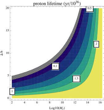
Figure 13: Proton lifetime with gauge boson mass $M_{X}=M_{\rm GUT}\simeq 2\cdot 10^{16}$ GeV. The grey region corresponds to the current exclusion limit.

6 Conclusions

In this paper we have studied the phenomenological consequences of the presence of new physics at a scale intermediate between the EW and the GUT scale in a SUSY theory. We have assumed that the new physics consists only of chiral superfields in complete GUT multiplets, such to maintain gauge coupling unification.

The main effect, which drives all the others, is the increment of the value of the unified gauge coupling. The simple requirement that it remains perturbative up to the GUT scale is already enough to exclude a large portion of the parameter space, as we have shown in Fig. 2. As a consequence of this increase, the entire low energy spectrum is modified with respect to the MSSM one and, in particular, the ratio of scalar over gaugino masses is enhanced. This has interesting consequences both for what concerns the collider phenomenology and the neutralino dark matter.

We have analysed two main sets of collider observables that can give hints of the presence of the intermediate scale or, on the contrary, can be used to constrain it: the mass invariants defined in Eqs. (10)-(12) and the edges in cascade decays. By measuring the sparticle masses at the LHC and building the invariants, one can in principle disentangle if we are in the presence of a CMSSM-like spectrum or if intermediate scales are present or if high energy boundary conditions are not universal. The same can be done if independent measurements of sparticle masses and the position of the edges in the invariant masses in cascade decays are available. Still, if this is not the case, we have shown that the maximum number of edges in these decays can give uncontroversial information that can be used to constrain the intermediate scale physics.

On the other hand, the generic increase of the ratio of scalar over gaugino masses tends to destabilise the regions of the parameters space where the correct DM relic density is obtained thanks to an efficient (co)annihilation of the lightest neutralino. This is the case for the $\tilde{\tau}$-coannihilation region or the A-funnel one: we have shown that the presence of the intermediate scale can render impossible to realise the precise relations among the masses of the involved particles necessary to enhance the (co)annihilation cross section. On the contrary, in spite of the presence of the intermediate scale, we found that it is always possible to find regions in the parameter space where the Higgsino-component of the neutralino is enough to increase the annihilation cross section and obtain the correct relic density (“focus-point” region).

Finally, we have observed that the increment of the unified gauge coupling can reduce the proton lifetime if the decay is driven by the GUT gauge bosons. We have shown that, for gauge boson masses equal to the GUT scale, the actual bound can be used to exclude a small part of the parameter space.

Appendix A Analytical one-loop formulae

In this section we collect analytical formulae that can be used to illustrate the effect of the intermediate scale on the renormalization group evolution of the MSSM parameters (see Sections 2). Aiming at compact and simply readable expressions, we consider, besides gauge couplings and gaugino masses, only first generations sfermion masses, for which Yukawa couplings can be neglected. Even though it is possible to obtain analytical solutions of the stop and Higgs masses as well, they result quite involved, hence we prefer to study these parameters numerically.

We first write the solution of the (one loop) gauge coupling RGEs in presence of fields at $M_{I}$ giving a contribution $\Delta b=\sum_{i}n_{i}$ (with $n_{i}$ being the Dynkin index of the SU(5) representation of the $i$-th field) to the $\beta$-function coefficients:

$$\frac{1}{\alpha_{i}(\mu)}=\left\{\begin{array}[]{lr}\frac{1}{\alpha_{U}}-\frac{b_{i}}{2\pi}\ln\frac{\mu}{M_{\rm GUT}}\,,&~{}~{}\mu>M_{I}\\ \frac{1}{\alpha_{U}}-\frac{\Delta b}{2\pi}\ln\frac{M_{I}}{M_{\rm GUT}}-\frac{b^{0}_{i}}{2\pi}\ln\frac{\mu}{M_{\rm GUT}}\,,&~{}~{}\mu<M_{I}\end{array}\right.$$ (22)

where $b^{0}_{i}$ are the ordinary MSSM coefficients

$$(b^{0}_{1},b^{0}_{2},b^{0}_{3})=(33/5,1,-3),~{}~{}~{}b_{i}=b_{i}^{0}+\Delta b\,,$$ (23)

and

$$\frac{1}{\alpha_{U}}=\frac{1}{\alpha_{i}(M_{S})}-\frac{b^{0}_{i}}{2\pi}\ln\frac{M_{\rm GUT}}{M_{S}}-\frac{\Delta b}{2\pi}\ln\frac{M_{\rm GUT}}{M_{I}}\,,$$ (24)

$$\ln\frac{M_{\rm GUT}}{M_{S}}=\frac{2\pi}{b^{0}_{i}-b^{0}_{j}}\left(\frac{1}{\alpha_{i}(M_{S})}-\frac{1}{\alpha_{j}(M_{S})}\right)\,.$$ (25)

Analogously for the gaugino masses we have:

$$M_{i}(\mu)=\left\{\begin{array}[]{lr}M_{i}(M_{\rm GUT})/\left(1-\frac{b_{i}}{2\pi}\alpha_{U}\ln\frac{\mu}{M_{\rm GUT}}\right)\,,&~{}~{}\mu>M_{I}\\ M_{i}(M_{\rm GUT})/\left(1-\frac{\Delta b}{2\pi}\alpha_{U}\ln\frac{M_{I}}{M_{\rm GUT}}-\frac{b^{0}_{i}}{2\pi}\alpha_{U}\ln\frac{\mu}{M_{\rm GUT}}\right)\,,&~{}~{}\mu<M_{I}\end{array}\right.$$ (26)

In particular, we have:

$$M_{i}(M_{S})= \frac{M_{i}(M_{\rm GUT})}{\alpha_{U}}\,\alpha_{i}(M_{S})$$

$$= M_{i}(M_{\rm GUT})\left(1-\frac{b^{0}_{i}}{2\pi}\alpha_{i}(M_{S})\ln\frac{M_{\rm GUT}}{M_{S}}-\frac{\Delta b}{2\pi}\alpha_{i}(M_{S})\ln\frac{M_{\rm GUT}}{M_{I}}\right)\,.$$ (27)

For the scalar masses, if we neglect Yukawa and A-term contributions, the solution in general looks like:

$$m^{2}_{\phi}(\mu)=m^{2}_{\phi}(M_{\rm GUT})+K_{1}(\mu)+K_{2}(\mu)+K_{3}(\mu)\,,$$ (28)

with

$$K_{i}(\mu)=C_{i}\frac{2}{\pi}\int_{\mu}^{M_{\rm GUT}}\alpha_{i}(\mu^{\prime})|M_{i}(\mu^{\prime})|^{2}d\mu^{\prime}\,,$$ (29)

and for the quadratic Casimirs $C_{i}$ we have: $C_{1}=3/5\,\mathcal{Y}_{\phi}^{2}$, with $\mathcal{Y}_{\phi}$ the hypercharge of $\phi$, $C_{2}=3/4~{}(0)$ for SU(2) doublets (singlets), $C_{3}=4/3~{}(0)$ for SU(3) triplets (singlets).

Using Eqs. (22, 26), we can easily solve the integrals and we get for $\mu<M_{I}$ (in particular $\mu=M_{S}$):

$$K_{i}(\mu)= 2C_{i}~{}M_{i}^{2}(M_{\rm GUT})~{}\left[\frac{1}{b_{i}}\left(1-\frac{1}{\left(1-\frac{b_{i}}{2\pi}\alpha_{U}\ln\frac{M_{I}}{M_{\rm GUT}}\right)^{2}}\right)+\right.$$

$$\left.\frac{1}{b^{0}_{i}}\left(\frac{1}{\left(1-\frac{b_{i}}{2\pi}\alpha_{U}\ln\frac{M_{I}}{M_{\rm GUT}}\right)^{2}}-\frac{1}{\left(1-\frac{\Delta b}{2\pi}\alpha_{U}\ln\frac{M_{I}}{M_{\rm GUT}}-\frac{b_{i}^{0}}{2\pi}\alpha_{U}\ln\frac{\mu}{M_{\rm GUT}}\right)^{2}}\right)\right]$$

$$= \frac{2C_{i}}{b^{0}_{i}}\left[\frac{b^{0}_{i}}{b_{i}}M_{i}^{2}(M_{\rm GUT})+\frac{\Delta b}{b_{i}}M_{i}^{2}(M_{I})-M_{i}^{2}(\mu)\right]\,.$$ (30)

Appendix B Effect of two-loop RGEs

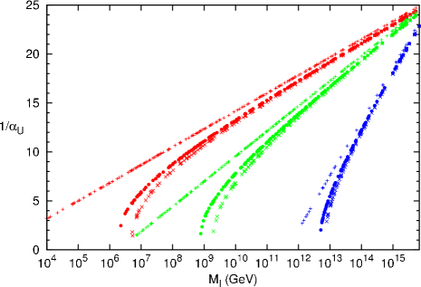
Figure 14: Effect of two loop running on $1/\alpha_{U}$. The red points correspond to $\Delta b=5$, the green ones to $\Delta b=7$ and the blue ones to $\Delta b=15$. In the three cases, the crosses correspond to one loop results, the diagonal crosses correspond to the two loop result with $n_{24}=1$ (red), $n_{15}=1$ (green) and $n_{24}=3$ (blue) and the dots show the two loop result considering only an appropriate number of ${\bf 5+\overline{5}}$.

At two loops, the RGE for the gauge couplings read:

$$\frac{d}{dt}g_{i}=\frac{g_{i}^{3}}{(4\pi)^{2}}\,b_{i}+\frac{g_{i}^{3}}{(4\pi)^{4}}\,\left(\sum_{i}b^{(2)}_{ij}\,g_{j}^{2}-\sum_{x}C_{i}^{x}y_{x}^{2}\right),$$ (31)

where the two loop $\beta$-function coefficients for the MSSM can be found, for instance, in Ref. [28]. Unlike in the one loop case, the new contribution depends in principle on the exact field content at the intermediate scale. For instance, we have:

$$\Delta b^{(2)}=$$ (32)

$$\left(\begin{array}[]{ccc}\frac{7}{15}n_{5}+\frac{23}{5}n_{10}+\frac{181}{15}n_{15}+\frac{25}{3}n_{24}&\frac{9}{5}n_{5}+\frac{3}{5}n_{10}+\frac{147}{5}n_{15}+15n_{24}&\frac{32}{15}n_{5}+\frac{48}{5}n_{10}+\frac{656}{15}n_{15}+\frac{80}{3}n_{24}\\ \frac{3}{5}n_{5}+\frac{1}{5}n_{10}+\frac{49}{5}n_{15}+5n_{24}&7n_{5}+21n_{10}+69n_{15}+45n_{24}&16n_{10}+16n_{15}+16n_{24}\\ \frac{4}{15}n_{5}+\frac{6}{5}n_{10}+\frac{82}{15}n_{15}+\frac{10}{3}n_{24}&6n_{10}+6n_{15}+6n_{24}&\frac{34}{3}n_{5}+34n_{10}+\frac{358}{3}n_{15}+\frac{230}{3}n_{24}\end{array}\right)\,,$$ (36)

where $n_{x}$ ($x=5,10,15,24$) denotes the number of ${\bf 5+\overline{5}}$, ${\bf 10+\overline{10}}$, ${\bf 15+\overline{15}}$ and ${\bf 24}$ representations at $M_{I}$, respectively.

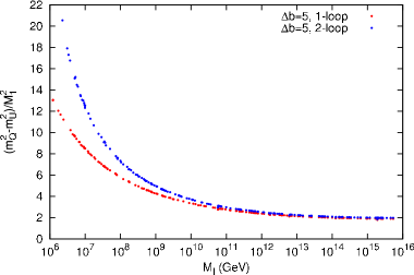
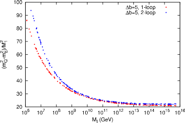
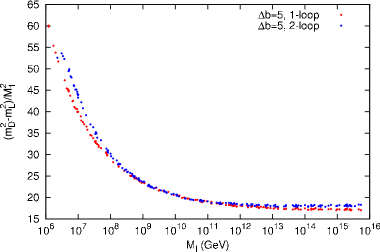
Figure 15: Effect of two loop running on the invariants $\Delta^{QU}$, $\Delta^{QE}$, $\Delta^{DL}$ for $\Delta b=5$ and $M_{S}=1$ TeV. The red points correspond to one loop RGEs, while the blue ones to two loops.

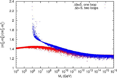
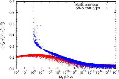
Figure 16: Effect of two loop running on the invariants $\Delta^{QE}_{DL}$ and $\Delta^{QU}_{DL}$ for $\Delta b=5$ with variable $M_{S}$. The red points correspond to one loop RGEs, while the blue ones to two loops.

The effect of two loop RGEs is illustrated in Fig. 14, where the cases $\Delta b=5$ (red), $\Delta b=7$ (green) and $\Delta b=15$ (blue) are compared. In the three cases, the crosses correspond to $1/\alpha_{U}$ vs. $M_{I}$ at one loop. The diagonal crosses correspond to the two loop result with the following field contents: $n_{24}=1$ (red), $n_{15}=1$ (green) and $n_{24}=3$ (blue). Finally, the dots show the two loop result considering only an appropriate number of $\bf 5+\overline{5}$, i.e. $n_{5}=\Delta b$. As we can see, the difference between “one loop equivalent” field contents (e.g. $1\times{\bf 24}$ and $5\times({\bf 5+\overline{5}})$) is appreciable only close to the Landau pole. Therefore, the two loop effects are to a very good approximation independent of the exact field content and we are going to implement the two loop RGEs taking always $n_{5}=\Delta b$.

In the second panel of Fig. 2, $1/\alpha_{U}$ is shown in the $\Delta b-M_{I}$ plane. We can see that $\alpha_{U}$ increases with respect to the one loop case. Therefore, we expect all the effects discussed in the paper to be further enhanced at two loops. For illustration, we show in Fig. 15 a comparison between the one loop and the two loops results for the mass invariants $\Delta_{i}^{ff^{\prime}}$ discussed in section 3 for $\Delta b=5$ and $M_{S}=1$ TeV. The two loop correction is mild (typically $\lesssim 10\%$) and grows close the Landau pole as expected. The two loop effect can be much more dramatic in the case of the quantities $\Delta_{f_{3}f_{4}}^{f_{1}f_{2}}$ defined in Eq. (12). This is depicted in Fig. 16 again for $\Delta b=5$ and a variation of the SUSY scale $M_{S}\lesssim 2$ TeV. While $M_{S}$ has no strong impact on the mass invariants (contrary to $\Delta_{i}^{ff^{\prime}}$), the two loop contribution can largely increase the effect of the intermediate scale on the quantities $\Delta_{f_{3}f_{4}}^{f_{1}f_{2}}$. Therefore the one loop expressions used for Fig. 8 just provide a (conservative) estimate in the regimes where the effect is mild and two loop RGEs should be taken into account for precise quantitative studies of this kind of observables.

References

- [1] M. Magg and C. Wetterich, Phys. Lett. B 94, 61 (1980); J. Schechter and J. W. F. Valle, Phys. Rev. D 23 (1981) 1666; C. Wetterich, Nucl. Phys. B 187, 343 (1981); G. Lazarides, Q. Shafi and C. Wetterich, Nucl. Phys. B 181, 287 (1981); R. N. Mohapatra and G. Senjanovic, Phys. Rev. D 23, 165 (1981).
- [2] R. Foot, H. Lew, X. G. He and G. C. Joshi, Z. Phys. C 44, 441 (1989).
- [3] A review on the three types of tree-level seesaw can be found in A. Abada, C. Biggio, F. Bonnet, M. B. Gavela and T. Hambye, 061 [arXiv:0707.4058 [hep-ph]].
- [4] C. D. Froggatt and H. B. Nielsen, Nucl. Phys. B 147 (1979) 277; M. Leurer, Y. Nir, N. Seiberg, Nucl. Phys. B398 (1993) 319-342 [hep-ph/9212278]; M. Leurer, Y. Nir, N. Seiberg, Nucl. Phys. B420, 468-504 (1994) [hep-ph/9310320].
- [5] L. Calibbi, Z. Lalak, S. Pokorski and R. Ziegler, arXiv:1203.1489 [hep-ph].
- [6] J. C. Pati and A. Salam, Phys. Rev. D 10 (1974) 275 [Erratum-ibid. D 11 (1975) 703].
- [7] R. N. Mohapatra and J. C. Pati, Phys. Rev. D 11 (1975) 2558; G. Senjanovic and R. N. Mohapatra, Phys. Rev. D 12 (1975) 1502.
- [8] L. Calibbi, L. Ferretti, A. Romanino, R. Ziegler, Phys. Lett. B672, 152-157 (2009) [arXiv:0812.0342 [hep-ph]].
- [9] M. R. Buckley and H. Murayama, Phys. Rev. Lett. 97 (2006) 231801 [hep-ph/0606088].
- [10] C. Biggio and L. Calibbi, JHEP 1010 (2010) 037 [arXiv:1007.3750 [hep-ph]].
- [11] J. N. Esteves, J. C. Romao, M. Hirsch, F. Staub and W. Porod, Phys. Rev. D 83 (2011) 013003 [arXiv:1010.6000 [hep-ph]].
- [12] V. De Romeri, M. Hirsch and M. Malinsky, Phys. Rev. D 84 (2011) 053012 [arXiv:1107.3412 [hep-ph]].
- [13] J. N. Esteves, J. C. Romao, M. Hirsch, W. Porod, F. Staub and A. Vicente, arXiv:1109.6478 [hep-ph].
- [14] J. N. Esteves, S. Kaneko, J. C. Romao, M. Hirsch and W. Porod, Phys. Rev. D 80 (2009) 095003 [arXiv:0907.5090 [hep-ph]].
- [15] L. Calibbi, M. Frigerio, S. Lavignac and A. Romanino, JHEP 0912 (2009) 057 [arXiv:0910.0377 [hep-ph]].
- [16] A. Rossi, Phys. Rev. D 66, 075003 (2002) [arXiv:hep-ph/0207006].
- [17] P. Fileviez Perez, Phys. Rev. D 76, 071701 (2007) [arXiv:0705.3589 [hep-ph]].
- [18] G. F. Giudice and R. Rattazzi, Phys. Rept. 322 (1999) 419 [hep-ph/9801271].
- [19] K. L. Chan, U. Chattopadhyay and P. Nath, Phys. Rev. D 58, 096004 (1998) [arXiv:hep-ph/9710473]; J. L. Feng, K. T. Matchev and T. Moroi, Phys. Rev. Lett. 84, 2322 (2000) [arXiv:hep-ph/9908309]; J. L. Feng, K. T. Matchev and F. Wilczek, Phys. Lett. B 482, 388 (2000) [arXiv:hep-ph/0004043].
- [20] H. Baer, V. Barger, A. Lessa, X. Tata, JHEP 1006, 102 (2010). [arXiv:1004.3594 [hep-ph]].
- [21] I. Hinchliffe, F. E. Paige, M. D. Shapiro, J. Soderqvist and W. Yao, Phys. Rev. D 55 (1997) 5520 [hep-ph/9610544]; H. Bachacou, I. Hinchliffe and F. E. Paige, Phys. Rev. D 62, 015009 (2000) [arXiv:hep-ph/9907518].
- [22] J. R. Ellis, T. Falk and K. A. Olive, Phys. Lett. B 444, 367 (1998) [arXiv:hep-ph/9810360]; J. R. Ellis, T. Falk, K. A. Olive and M. Srednicki, Astropart. Phys. 13, 181 (2000) [Erratum-ibid. 15, 413 (2001)] [arXiv:hep-ph/9905481].
- [23] M. Drees and M. M. Nojiri, Phys. Rev. D 47, 376 (1993) [arXiv:hep-ph/9207234].
- [24] L. Calibbi, A. Faccia, A. Masiero and S. K. Vempati, Phys. Rev. D 74 (2006) 116002 [hep-ph/0605139].
- [25] L. Calibbi, Y. Mambrini and S. K. Vempati, JHEP 0709 (2007) 081 [arXiv:0704.3518 [hep-ph]].
- [26] H. Nishino, K. Abe, Y. Hayato, T. Iida, M. Ikeda, J. Kameda, Y. Koshio and M. Miura et al., arXiv:1203.4030 [hep-ex].
- [27] J. Hisano, D. Kobayashi and N. Nagata, arXiv:1204.6274 [hep-ph].
- [28] S. P. Martin and M. T. Vaughn, Phys. Rev. D 50 (1994) 2282 [Erratum-ibid. D 78 (2008) 039903] [hep-ph/9311340].