The , , and mesons in a double pole QCD Sum Rule
Abstract
We use the method of double pole QCD sum rule which is basically a fit with two exponentials of the correlation function, where we can extract the masses and decay constants of mesons as a function of the Borel mass. We apply this method to study the mesons: , , and . We also present predictions for the toponiuns masses of and .
pacs:
14.40.Pq, 13.20.GdI Introduction
In 1977, Shifman, Vainshtein, Zakharov, Novikov, Okun and Voloshin Novikov:1977dq ; Novikov:1977cm ; Shifman:1978bx ; Shifman:1978zq created the successful method of QCD sum rules (QCDSR), which is widely used nowadays. With this method, we can calculate many hadron parameters such as: mass of the hadron, decay constant, coupling constant and form factors in terms of the QCD parameters as for example: quark masses, the strong coupling and non-perturbative parameters like quark condensate and gluon condensate. The main point of this method is that the quantum numbers and content of quarks in hadron are represented by an interpolating current, where the correlation function of this current is introduced in the framework of the operator product expansion (OPE). To determine the mass and the decay constant of the ground state of the hadron, we use the two point correlation function. On the QCD side, the correlation function can be written in terms of a dispersion relation and on the phenomenological side can be written in terms of the ground state and several excited states. The usual QCDSR method uses an ansatz that the phenomenological spectral density can be represented by a form pole plus continuum, where is assumed that the phenomenological and QCD spectral density coincides with each other above the continuum threshold. The continuum is represented by an extra parameter called, , as being correlated with the onset of excited states Colangelo:2000dp . In general, the resonance activity occurs with lower than the mass of the first excited state.
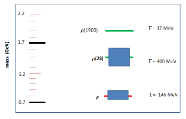
For the meson spectrum, Fig.(1), the purpose of pole plus continuum is a good approach, due to the large decay width of the or , that allow to approximate the excited states as a continuum.
For the meson Reinders:1984sr the value of that best fit the mass and the decay constant is GeV and for the meson the value is . We note that the values quoted above for are of about 250 MeV below of the poles of and . One interpretation of this result, it is due to the effect of the large decay width of these mesons.
The pioneering work on charmonium sum rule, Novikov et al. Novikov:1977dq considered the phenomenological side with double pole and GeV, where is double pole continuum parameter. This value is correlated with the threshold of pair production of charmed mesons. Using this value of and Moment Sum Rule at , they presented the first estimate for the gluon condensate and a nice prediction of the mass of 3.0 GeV, while the experimental results in 1977 reported a mass of 2.83 GeV Novikov:1977dq ; Novikov:1977cm ; Shifman:1978zq .
In single pole sum rule for and , the best values of that fit the masses are GeV Reinders:1984sr , where the minimum value of is 100 MeV below of the mass. As the decay width of the is about 0.3 MeV, so it is approximate to associate the parameter with some activity of excited states.
In principle the value of can be fixed by setting the mass of the ground state, on the other hand, in the case where the mass of the ground state is unknown as in the case of tetraquarks, there are studies that extract the lower limit of , since the pole dominance and OPE convergence is controlled Bracco:2008jj .
In double pole QCDSR Shifman:1978zq , we expect that a reliable sum rule should provide that the ground state decay constant is larger than the excited state decay constant and provides an upper limit of , as we can see in our results. This condition is directly related with the expression of decay constant obtained from potential models Zakharov:1975ku ; Segovia:2014mca ; Lakhina:2006vg is proportional to the meson wave function at the origin. As the meson radius increases with excitation, the probability of finding its quarks at the origin declines with the excitation Leinweber:1994gt . This condition was used by Shifman Shifman:1978zq to predict the mass of the and this condition agrees with the experimental data from the spectrum of and up to pdg.2012 . For is observed a violation in this behavior, where the decay constant of is larger than . This result is not predicted by potential models and the authors of Ref.Segovia:2014mca suggest that the could be a tetraquark or molecule state.
In QCDSR, the excited states are studied in: pole-pole plus continuum in Moment Sum Rule at Novikov:1977dq ; Novikov:1977cm , the spectral sum rules with pole-pole-pole plus continuum Singh:2006ii , the Maximum Entropy Method Gubler:2010cf and Gaussian Sum Rule with pole-pole plus continuum ansatz Harnett:2008cw . There are studies on the mesons Gubler:2010cf ; Bakulev:1998pf ; Pimikov:2013usa , nucleons Singh:2006ii ; Ohtani:2011yy , mesons Novikov:1977cm , mesons Novikov:1977dq ; Gubler:2011ua and mesons Suzuki:2012ze . In Gaussian Sum Rule is studied the mixed states of the glueballs and scalar mesons. In lattice QCD, there are studies on the mesons McNeile:2006qy , mesons excited states Burch:2004he ; Yamazaki:2001er , charmonium Dudek:2006ej ; Dudek:2007wv ; Liu:2011rn , nucleons excited states Mathur:2003zf ; Edwards:2011jj ; Leinweber:1994gt ; Guadagnoli:2004wm and exotic charmonium spectrum Liu:2012ze . In addition, the excited states have been studied recently by several approaches like: QCD Bethe-Salpeter equation Qin:2011xq for and , light-front quark model Peng:2012tr ; Arndt:1999wx for , , and the bottomonium analogous. The has been studied in QCDSR as a hybrid meson Kisslinger:2009pw using the pole plus continuum ansatz.
The method pole-pole plus continuum ansatz was used in lattice QCD for nucleons Leinweber:1994gt . The authors have shown a problem in which the ground state coupling strength is lower than the excited state coupling strength.
There are many motivations to study the excited states that belong the charmonium spectrum. New charmonium-like states Y(4260) and Y(4660) are an example of the importance of excited states. When considering theories that Y(4260) has been proposed as a bound state of MartinezTorres:2009xb and Y(4660) has been interpreted as a bound state of , Wang:2009hi ; Albuquerque:2011ix ; Guo:2008zg , where we can speculate that Y(4660) is an excited state of Y(4260). Another point is that could be an excited state of and could be an excited state of Navarra:2011xa .
In this paper, we study the excited state using the pole-pole plus continuum ansatz in QCD sum rules and we apply in four cases: the , , and mesons and we calculate their masses and decay constants.
II The Sum Rule
In the determination of the mass and the decay constant with QCDSR, we use the two point correlation function Shifman:1978bx ,
| (1) |
where on the QCD point of view, the current of vector mesons has the form:
| (2) |
Inserting this current in the correlation function, Eq.(1), are obtained the operators expansion, OPE, which can be written in terms of a dispersion relation which depends on the QCD parameters, then the correlator can be written in the form:
| (3) |
with:
| (4) |
where and the parameter is the minimum value of to have an imaginary part of the perturbative term and the correlator is the contribution of the condensates.
On the phenomenological side, we use:
| (5) |
| (6) |
We can write the invariant part of the correlator of the Eq.(6) in the form:
| (7) |
with
| (8) |
and .
When comparing the Eq.(3) with Eq.(7) the simplest way to perform the sum rule is choosing an invariant structure and equating both sides of the sum rule, so we have:
| (9) |
Finally, we obtain the sum rule:
| (10) |
To improve the equivalence between the two sides of the sum rule is convenient to use the Borel transformation Shifman:1978bx :
| (11) |
with and , where M is Borel mass.
For the sum rule of meson we use and are given by Shifman:1978bx ; Reinders:1984sr ; Colangelo:2000dp :
| (12) |
| (13) |
where is the strong coupling constant, is light quark mass, is gluon condensate, is quark condensate, and . We use these parameters at GeV renormalization scale Colangelo:2000dp .
For the sum rules of and mesons we use and are given by Reinders:1984sr ; Novikov:1977dq .
| (14) |
where,
| (15) |
| (16) |
with and m is off-shell heavy quark mass and .
For the gluon condensate we apply the Borel transform of the expression was given by Reinders et al. Reinders:1984sr , where we have:
| (17) |
III The Method
To implement our method, we consider the following spectral density on the phenomenological side:
| (18) |
where is the mass of the ground state and is the mass of the first excited state, coupling strength is the decay constant for the ground state and is the decay constant for the first excited state and mark the onset of the continuum states. Inserting Eq.(18) on the left hand side of Eq.(11), we get the expressions:
| (19) |
On the right hand side of Eq.(11), we get:
| (20) |
Equating Eq.(19) with Eq.(20) and using the quark hadron duality, where we assume that for , so we get the double pole QCD sum rule,
| (21) |
where,
| (22) |
The contribution of the resonances is given by:
| (23) |
As usually done in QCDSR, the obtaining mass of the hadron, we take the derivative of Eq.(21) with respect to and we get the new equation:
| (24) |
| (25) |
| (26) |
Solving the equation system Eq.(21) and Eq.(24) writings in terms of the functions and , we easily get:
| (27) |
| (28) |
where we use the notation
| (29) |
To eliminate the dependence of the coupling in Eq.(27), we take a derivative of this equation with respect of and divide the result by Eq.(27). The result of this procedure is given by the Eq.(30). The procedure to eliminate coupling is analogous that used above and the result is given by the Eq.(31).
| (30) |
| (31) |
In the first view the Eq.(30) and Eq.(31) suggest a system for the masses and , that could be extracted the masses. On the other hand, using Eq.(30) to obtain a expression, it reproduces the same result has given in Eq.(31). To solve this problem of cannot decouple the masses and , we will take the derivative of equation Eq.(28) twice in the form:
| (32) |
Dividing by equation Eq.(28) we have a new mass formula, is given by:
| (33) |
| (34) |
where , , and .
For obtaining , we can do the same procedure as above and obeys the same equation Eq.(34). Thus, we easily solved this equation in which the mass of the ground state and the excited state are given by:
| (35) |
| (36) |
IV Results
In this work we use the following parameters for meson: , , at GeV renormalization scale Colangelo:2000dp . For , we use the , and for , we use the , .
In addition to the above mentioned parameters, the sum rule depends of the others two parameters: the continuum threshold and the Borel mass, M.
As explained in the introduction, we expect that is a value closes to (3S) meson mass, however, in cases where the 3S state is unknown or has large decay width, the value of is limited by the condition that the decay constant of 2S meson should be smaller than 1S meson and the lowest limit of is considered as m(2S) + 100 MeV.
Using a value of , the range of Borel mass is chosen on the assumption that the ratio of the double pole Eq.(21) and the total contribution pole-pole plus the resonances, Eq.(23), should be higher than .
IV.1 Sum Rule
Using the mass of meson of , Fig.(1), we test , but in this case the decay constant of excited state is larger than the of the ground state, so the sum rule fails.
The maximum value of is 1.66 GeV, where in this case the decay constant of excited state is slightly below of the decay constant of ground state. The minimum value of is 1.56 GeV, because - m(2S) reaches the value of 100 MeV.
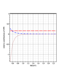
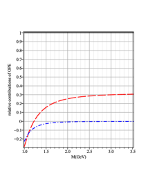
In Fig.(2) the contribution of the OPE terms are ordered relative to the first order perturbative term of Eq.(12) in Eq.(22). The solid line is the contribution of the first order perturbation term is adopted as 1, long-dashed line is the radiative correction, dashed-dot line is the dimension 4 of Eq.(13) and dot is the dimension 6 of Eq.(13). We note that the convergence of OPE is controlled and at M=1 GeV, the contributions of the dimension 4 is 1.82% and dimension 6 is 2.26% of the first order perturbation term. For M=2 GeV, these condensates contribute with 300 MeV in the mass of and 100 MeV for the mass of .
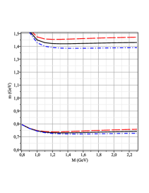
We study the behavior of the masses and decay constants of the mesons and as a function of Borel mass for three values : solid line for , dashed-dot line for and long-dashed line for . We can see in Fig.(3) that all masses are stable and at M=1.2 GeV, the long-dashed line gives a value compatible with the experimental value for the mass of 1454 MeV and for the the long-dashed line gives a mass of 740 MeV.
For the calculation of the decay constant, we use the experimental values GeV and GeV. In Fig.(4), we show the decay constant of the and mesons. Considering the value for of 1.61 GeV (solid line), the value of the meson decay constant has a plateau on value 203 MeV and has a plateau on the value 186 MeV. Considering uncertainty with respect to parameter at M= 2 GeV, we get:
| (37) |
| (38) |
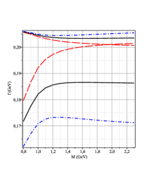
The value of is 17 MeV lower than the experimental value of MeV pdg.2012 obtained from decay width considering .
It is interesting to note that in Ref. Becirevic:2003pn show another way to extract the experimental decay constant of the from semileptonic decay, . Using the PDG pdg.2012 , we get:
| (39) |
IV.2 Sum Rule
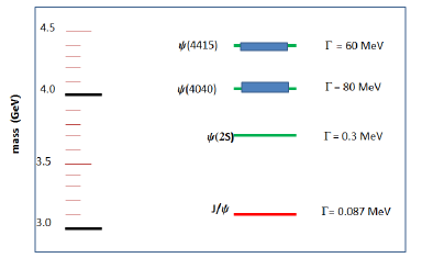
Using the mass of meson of , Fig.(1), we consider , but in this case the decay constant of the excited state is larger than the ground state decay constant, so the sum rule fails.
The maximum value of is 3.9 GeV, where in this case the decay constant of the excited state is slightly below the decay of ground. The minimum value of is 3.7 GeV, because - m(2S) reaches the value of 100 MeV.
It is also interesting that the mass of the (1S) state is almost independent on the value of in stable Borel range, even varying 3.3 GeV to , furthermore mass (2S) state increases with the increasing of , but assumes a maximum value of 4.1 GeV.
In Fig.(5), the contribution of the OPE terms are ordered relative to the first order perturbative term of Eq.(14) in Eq.(22). The solid line is the contribution of the first order perturbation term is adopted as 1, long-dash line is the radiative correction, dash-dot line is the gluon condensate of Eq.(17). We note that the convergence of OPE is controlled and the contribution of the gluon condensate is 6% of the first order perturbation term at M=1.4 GeV, the same order of radiative corrections. At M=2 GeV its contribution reduces to only 1% of the first order perturbation term.
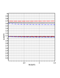
We study the behavior of the mass of meson and as a function of Borel mass for three values . We have in Fig.(6), solid line for , dashed-dot line for and long-dashed line for .
We can see in Fig.(6) that all masses are stable at GeV and the solid line is for the mass of 3.07 GeV and mass of 3.64 GeV.
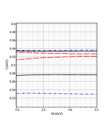
For the calculation of the decay constant, we use the experimental values and . In Fig.(7) we can see that the decay constants are stable GeV. Considering uncertainty with respect to parameter at GeV, we get:
| (40) |
and for meson decay constant, we get: .
The result for the decay constant of is in agreement with the experimental value of of MeV pdg.2012 obtained from decay width considering . For , the decay constant is 82 MeV lower than the experimental value of of MeV.
IV.3 Sum Rule
Using the mass of meson of , Fig.(1), we consider .
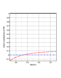
In Fig.(8), the contribution of the OPE terms are ordered relative to the first order perturbative term of Eq.(14) in Eq.(22). The solid line is the contribution of the first order perturbation term is adopted as 1, long-dashed line is the radiative correction, dashed-dot line is the gluon condensate of Eq.(17). We note that the convergence of OPE is controlled and the contribution of the gluon condensate is only 0.05% of the first order perturbation term at M=5 GeV and 0.01% at M=7 GeV.
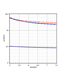
We study the behavior of the mass of and as a function of Borel mass for three values of . We can see in Fig.(9), solid line for , dashed-dot line for and longer dashed line for .
We can see in Fig.(9) that all masses are stable at GeV. At M=6.5 GeV, the mass obtained for is 9.46 GeV and is 200 MeV above of the experimental value.
For the calculation of the decay constant, we use the experimental values , . In Fig.(10) we see that the values for the decay constant have good stability for a Borel mass above 6 GeV.
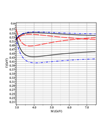
Considering uncertainty with respect to parameter at GeV, we get:
| (41) |
For the meson decay constant, we get: .
IV.4 toponium meson Sum Rule
In this case, we show how to use our method to predict particles not yet discovered as compound of top quark. One problem of this sum rule is that correction O() is important, making this sum rule less reliable than the . There are papers that are against the existence of the toponium Fabiano:1993vx and papers in favor Ref.Kiyo:2002rr ; Goncharov:2008fh where they have predicted a mass of and with a mass of 347.4 GeV.
In this case is chosen to satisfy ordering of decay constants and the condition is of about 100 MeV. However, we prefer to relax this condition to , due the variation of m(2S) as Borel mass in the scale of 1 GeV. We also consider the value of pdg.2012 , , where this value is close to the results of the Refs.KOKKAS:2014fla ; Abdallah:2004xe and the maximum value of the gluon condensate.
Initially, we attempt a value to as is shown in the first column of Tab.1, where the Borel window is limited between and , where the pole contribution is above 40% of total correlator and OPE convergence is controlled. The masses are calculated in distinct Borel windows. The decay constants are calculated at the midpoint . In the first attempt, we can see that the value led to a violation in the ordering of the decay constants, which leads us in the next attempt to use values of smaller than 1 TeV. Only in the third attempt, was obtained the ordering. Now we improve the gap between and m(2S) with a value of about 1 GeV, that is obtained in the final attempt.
Thus, we get the following results for the masses of of and .
| attempt 1 | attempt 2 | attempt 3 | attempt 4 | |
|---|---|---|---|---|
| 1000 | 450 | 376 | 375 | |
| 2000 | 200 | 100 | 100 | |
| 10000 | 1000 | 300 | 300 | |
| 540 | 364 | 357 | 357 | |
| 903 | 430 | 374 | 374 | |
| 103 | 27 | 18.9 | 18.7 | |
| 109 | 32 | 7.6 | 7.1 |
Finally, we collect all the results from the decay constant have obtained in this section in Tab.(2). In the column “this work” refers to the extraction of decay constants on the same Borel window. The “column experiment” refers to the average values of PDG pdg.2012 , to the process , considering .
| This work | Ref.Arndt:1999wx | Ref.Qin:2011xq | Ref.Peng:2012tr | lattice | lattice | experiment | |
|---|---|---|---|---|---|---|---|
| () | Ref.Yamazaki:2001er ; Dudek:2006ej | Ref.Jansen:2009hr ; Becirevic:2013bsa | Ref.pdg.2012 | ||||
| 216.37 | 268 | - | |||||
| 128 | 155 | - | - | - | |||
| - | - | - | |||||
| - | - | 371 | - | ||||
| - | - | 546.6 | - | - | |||
| - | - | 583.2 | - | - |
V Conclusions
In this work we have presented a method to QCD sum rule with double pole which is basically a fit with two exponentials of the correlation function, where we can extract the masses and decay constants of mesons as a function of the Borel mass. We study the mesons: , and , where we know their masses and decay constants from the experimental data, except the decay constant. We also study the hypothetica meson called toponium as an example how to use our method to predict new hadrons.
Using the experimental values for the meson masses, the decay constants have a good stability as Borel mass and we have shown a prediction for the decay constant of MeV.
In addition, the decay constants of and have value lower than the experimental values.
We finish with an application of this method to study the hypothetical particle called toponium. In this case, we start with an initial tentative value for the continuum threshold using a very high initial value of 1 TeV and we note that the ordering of the decay constants is violated, which led us naturally to reduce the continuum threshold up to the minimum value of m(2S)+ 1 GeV. We use the lowest value of the continuum threshold to get the toponiuns masses of and .
VI Acknowledgements
We would like to thank Prof. Francisco de Assis de Brito for fruitful discussions. This work has been partially supported by CAPES.
References
- (1) V. A. Novikov, L. B. Okun, M. A. Shifman, A. I. Vainshtein, M. B. Voloshin and V. I. Zakharov, Phys. Rept. 41, 1 (1978).
- (2) V. A. Novikov, L. B. Okun, M. A. Shifman, A. I. Vainshtein, M. B. Voloshin and V. I. Zakharov, Phys. Lett. B 67, 409 (1977).
- (3) M. A. Shifman, A. I. Vainshtein and V. I. Zakharov, Nucl. Phys. B 147, 385 (1979).
- (4) M. A. Shifman, A. I. Vainshtein, M. B. Voloshin and V. I. Zakharov, Phys. Lett. B 77, 80 (1978).
- (5) P. Colangelo and A. Khodjamirian, In *Shifman, M. (ed.): At the frontier of particle physics, vol. 3* 1495-1576 [hep-ph/0010175].
- (6) B. Aubert et al. [BaBar Collaboration], Phys. Rev. D 77, 092002 (2008) [arXiv:0710.4451 [hep-ex]].
- (7) L. J. Reinders, H. Rubinstein and S. Yazaki, Phys. Rept. 127, 1 (1985).
- (8) M. E. Bracco, S. H. Lee, M. Nielsen and R. Rodrigues da Silva, Phys. Lett. B 671, 240 (2009) [arXiv:0807.3275 [hep-ph]].
- (9) W. Chen and S. L. Zhu, Phys. Rev. D 83, 034010 (2011) [arXiv:1010.3397 [hep-ph]].
- (10) V. I. Zakharov, B. L. Ioffe and L. B. Okun, Sov. Phys. Usp. 18, 757 (1975) [Usp. Fiz. Nauk 117, 227 (1975)].
- (11) J. Segovia, D. R. Entem and F. Fernandez, arXiv:1409.7079 [hep-ph].
- (12) O. Lakhina and E. S. Swanson, Phys. Rev. D 74 (2006) 014012 [hep-ph/0603164].
- (13) D. B. Leinweber, Phys. Rev. D 51, 6369 (1995) [nucl-th/9405002].
- (14) J. Beringer et al. (Particle Data Group), Phys. Rev. D 86, 010001 (2012).
- (15) J. P. Singh and F. X. Lee, Phys. Rev. C 76, 065210 (2007) [nucl-th/0612059].
- (16) P. Gubler and M. Oka, Prog. Theor. Phys. 124, 995 (2010) [arXiv:1005.2459 [hep-ph]].
- (17) D. Harnett, R. T. Kleiv, K. Moats and T. G. Steele, Nucl. Phys. A 850, 110 (2011) [arXiv:0804.2195 [hep-ph]].
- (18) A. P. Bakulev and S. V. Mikhailov, Phys. Lett. B 436, 351 (1998) [hep-ph/9803298].
- (19) A. V. Pimikov, S. V. Mikhailov and N. G. Stefanis, arXiv:1312.2776 [hep-ph].
- (20) K. Ohtani, P. Gubler and M. Oka, AIP Conf. Proc. 1343, 343 (2011) [arXiv:1104.5577 [hep-ph]].
- (21) P. Gubler, K. Morita and M. Oka, Phys. Rev. Lett. 107, 092003 (2011) [arXiv:1104.4436 [hep-ph]].
- (22) K. Suzuki, P. Gubler, K. Morita and M. Oka, arXiv:1204.1173 [hep-ph].
- (23) C. McNeile et al. [UKQCD Collaboration], Phys. Lett. B 642, 244 (2006) [hep-lat/0607032].
- (24) T. Burch et al. [Bern-Graz-Regensburg Collaboration], Phys. Rev. D 70, 054502 (2004) [hep-lat/0405006].
- (25) T. Yamazaki et al. [CP-PACS Collaboration], Phys. Rev. D 65, 014501 (2002) [hep-lat/0105030].
- (26) J. J. Dudek, R. G. Edwards and D. G. Richards, Phys. Rev. D 73, 074507 (2006) [hep-ph/0601137].
- (27) J. J. Dudek, R. G. Edwards, N. Mathur and D. G. Richards, Phys. Rev. D 77, 034501 (2008) [arXiv:0707.4162 [hep-lat]].
- (28) L. Liu, S. M. Ryan, M. Peardon, G. Moir and P. Vilaseca, arXiv:1112.1358 [hep-lat].
- (29) N. Mathur, Y. Chen, S. J. Dong, T. Draper, I. Horvath, F. X. Lee, K. F. Liu and J. B. Zhang, Phys. Lett. B 605, 137 (2005) [hep-ph/0306199].
- (30) R. G. Edwards, J. J. Dudek, D. G. Richards and S. J. Wallace, Phys. Rev. D 84, 074508 (2011) [arXiv:1104.5152 [hep-ph]].
- (31) D. Guadagnoli, M. Papinutto and S. Simula, Phys. Lett. B 604, 74 (2004) [hep-lat/0409011].
- (32) L. Liu, G. Moir, M. Peardon, S. M. Ryan, C. E. Thomas, P. Vilaseca, J. J. Dudek and R. G. Edwards et al., arXiv:1204.5425 [hep-ph].
- (33) S. -x. Qin, L. Chang, Y. -x. Liu, C. D. Roberts and D. J. Wilson, Phys. Rev. C 85, 035202 (2012) [arXiv:1109.3459 [nucl-th]].
- (34) T. Peng and B. -Q. Ma, arXiv:1204.0863 [hep-ph].
- (35) D. Arndt and C. -R. Ji, Phys. Rev. D 60, 094020 (1999) [hep-ph/9905360].
- (36) L. S. Kisslinger, Phys. Rev. D 79 (2009) 114026 [arXiv:0903.1120 [hep-ph]].
- (37) A. Martinez Torres, K. P. Khemchandani, D. Gamermann and E. Oset, Phys. Rev. D 80, 094012 (2009) [arXiv:0906.5333 [nucl-th]].
- (38) Z. G. Wang and X. H. Zhang, Commun. Theor. Phys. 54, 323 (2010) [arXiv:0905.3784 [hep-ph]].
- (39) R. M. Albuquerque, M. Nielsen and R. R. da Silva, Phys. Rev. D 84 (2011) 116004 [arXiv:1110.2113 [hep-ph]].
- (40) F. -K. Guo, C. Hanhart and U. -G. Meissner, Phys. Lett. B 665, 26 (2008) [arXiv:0803.1392 [hep-ph]].
- (41) F. S. Navarra, M. Nielsen and J. -M. Richard, J. Phys. Conf. Ser. 348, 012007 (2012) [arXiv:1108.1230 [hep-ph]].
- (42) S. Godfrey and N. Isgur, Phys. Rev. D 32, 189 (1985).
- (43) D. Ebert, R. N. Faustov and V. O. Galkin, Phys. Rev. D 79, 114029 (2009) [arXiv:0903.5183 [hep-ph]].
- (44) K. Morita and S. H. Lee, Phys. Rev. D 82, 054008 (2010) [arXiv:0908.2856 [hep-ph]].
- (45) T. DeGrand, Z. Liu and S. Schaefer, Phys. Rev. D 74, 094504 (2006) [Erratum-ibid. D 74, 099904 (2006)] [hep-lat/0608019].
- (46) T. Hambye, S. Peris and E. de Rafael, JHEP 0305, 027 (2003) [hep-ph/0305104]. Leupold:1997dg
- (47) S. Leupold, W. Peters and U. Mosel, Nucl. Phys. A 628, 311 (1998) [nucl-th/9708016].
- (48) D. Becirevic, V. Lubicz, F. Mescia and C. Tarantino, JHEP 0305, 007 (2003) [hep-lat/0301020].
- (49) C. McNeile, C. T. H. Davies, E. Follana, K. Hornbostel and G. P. Lepage, Phys. Rev. D 86, 074503 (2012) [arXiv:1207.0994 [hep-lat]].
- (50) J. Erler, Phys. Rev. D 59, 054008 (1999) [hep-ph/9803453].
- (51) S. Bodenstein, C. A. Dominguez, K. Schilcher and H. Spiesberger, Phys. Rev. D 86, 093013 (2012) [arXiv:1209.4802 [hep-ph]].
- (52) F. Klingl, N. Kaiser and W. Weise, Z. Phys. A 356, 193 (1996) [hep-ph/9607431].
- (53) N. Brambilla et al. [Quarkonium Working Group Collaboration], hep-ph/0412158.
- (54) P. Ruiz-Femenia and A. Pich, Phys. Rev. D 64, 053001 (2001) [hep-ph/0103259].
- (55) G. Abbiendi et al. [OPAL Collaboration], Eur. Phys. J. C 45, 1 (2006) [hep-ex/0505072].
- (56) N. Fabiano, A. Grau and G. Pancheri, Phys. Rev. D 50, 3173 (1994).
- (57) Y. Kiyo and Y. Sumino, Phys. Rev. D 67, 071501 (2003) [hep-ph/0211299].
- (58) Y. P. Goncharov, Nucl. Phys. A 808, 73 (2008) [arXiv:0806.4747 [hep-ph]].
- (59) P. Kokkas [CMS Collaboration], PoS EPS -HEP2013, 436 (2013).
- (60) J. Abdallah et al. [DELPHI Collaboration], Eur. Phys. J. C 37, 1 (2004) [hep-ex/0406011].
- (61) K. Jansen et al. [ETM Collaboration], Phys. Rev. D 80, 054510 (2009) [arXiv:0906.4720 [hep-lat]].
- (62) D. Becirevic, G. Duplancic, B. Klajn, B. Melic and F. Sanfilippo, Nucl. Phys. B 883, 306 (2014) [arXiv:1312.2858 [hep-ph]].