Probing for Invisible Higgs Decays with Global Fits
Abstract
We demonstrate by performing a global fit on Higgs signal strength data that large invisible branching ratios () for a Standard Model (SM) Higgs particle are currently consistent with the experimental hints of a scalar resonance with mass . For this mass, we find ( CL) from a global fit to individual channel signal strengths supplied by ATLAS, CMS and the Tevatron collaborations. Novel tests that can be used to improve the prospects of experimentally discovering the existence of a with future data are proposed. These tests are based on the combination of all visible channel Higgs signal strengths, and allow us to examine the required reduction in experimental and theoretical errors in this data that would allow a more significantly bounded invisible branching ratio to be experimentally supported. We examine in some detail how our conclusions and method are affected when a scalar resonance at this mass scale has couplings deviating from the SM ones.
I Introduction
Two outstanding questions of importance that the LHC should shed light on are the origin of electroweak symmetry breaking (EWSB), and the relationship of the mechanism of EWSB to new states beyond the Standard Model (SM).
There is strong indirect evidence for the EWSB sector being described by a theory that includes a particle that (at least) approximately has the properties of the SM Higgs boson. This evidence follows from many observables in flavour physics, from electroweak precision data (EWPD), LEP, the Tevatron and now the LHC. The SM Higgs is consistent with the results of these experimental probes in its pattern of breaking custodial symmetry () Susskind:1978ms ; Weinberg:1979bn ; Sikivie:1980hm as well as in the manner by which it sources the experimentally established pattern of flavour violation. In light of these results, there is substantial indirect evidence that a scalar field involved in EWSB will also be SM Higgs like in that the soft Higgs theorems of Refs. Shifman:1979eb ; Vainshtein:1980ea will be approximately respected, i.e. the scalar field will couple to the SM fields with a strength that is proportional to the mass of the corresponding SM particle.
Directly, LEP, the Tevatron and LHC have jointly excluded large regions of possible Higgs masses in the SM. The upper bound (in the low mass region) for the SM Higgs is now restricted to by ATLAS atlasnote2012019 and by CMS CMSnote12008 at CL, with a suggestive clustering of possible signal events around . However, in spite of these results, the Higgs hypothesis is not yet established. In particular, there remains a significant freedom in the allowed couplings of a scalar effective field to the SM gauge bosons and fermions - so long as such a resonance has the approximate symmetries and properties discussed above Carmi:2012yp ; Azatov:2012bz ; Espinosa:2012ir .111For other model independent approaches to Higgs couplings determination see Lafaye:2009vr ; Englert:2011aa ; Klute:2012pu . Such deviations in the properties of a scalar field from the SM Higgs can be interpreted as following from the Higgs boson emerging from a strongly interacting sector as a pseudo-Goldstone boson, or as the leading effect in the effective theory of more massive states that are integrated out.
In light of this experimental situation, attempting to use current (and future) Higgs signal strength parameters to establish relationships between the EWSB sector and beyond the SM states is speculative. This is certainly the current status, as the suggestive clustering of signal excesses at has not risen to the level of experimental evidence for a scalar resonance. Nevertheless, in this paper we will assume that future data will support the discovery of a scalar resonance at approximately this mass scale. Further, we will consider current signal strength measurements as indicative of the properties that such a scalar resonance has when performing global fits. In anticipation of such a discovery, it is of interest to consider how to efficiently extract evidence of yet other states coupled to such a scalar field.
The gauge invariant mass operator of the scalar degrees of freedom, being of dimension two, is expected to couple generally to all degrees of freedom. It is difficult to forbid a coupling of this operator at the renormalizable (or non-renormalizable) level to new states. As such, the measurement of the decay width of a new scalar resonance to states that do not directly lead to significant excesses in the Higgs discovery channels, defined in this paper as its invisible branching ratio , could be the first direct measurement of interactions with states beyond the SM. This exciting possibility has lead to many studies on extracting the invisible width of the Higgs. In this paper we will explore a very straightforward route using current and future experimental results on Higgs properties, expressed in terms of signal strength data, to probe for evidence of a . We first show (in Section II) that the current experimental hints of a new scalar resonance at do not put strong constraints on . We then explore in detail how to extract evidence for (or exclude) a using global combinations of best fit signal strength parameters, performing global fits, and demonstrating a global probability density function (PDF) approach that can be used to explore and optimize searches for in certain scenarios of beyond the SM (BSM) physics (Section II.1). In Section II.2, we examine the related issue of the precision with which is expected to be known in these scenarios when errors are small enough for a resonance discovery to be claimed.
These promising results raise the question of the robustness of such a global approach. These techniques are most promising when BSM physics couples to the SM primarily through the ‘Higgs portal’ Schabinger:2005ei ; Patt:2006fw ; Chang:2008cw ; MarchRussell:2008yu ; Espinosa:2007qk ; Pospelov:2011yp , i.e. they are optimal in BSM scenarios where new states are not charged under the SM gauge group and couple to the SM (initially) through the SM gauge singlet scalar mass operator. This is the case we explore in detail throughout Section II. We briefly discuss and summarize the prospects for global fits to uncover in broader scenarios in Section III where the effective couplings of the Higgs to the SM fields deviate from their SM values due to the Higgs being a pseudo-Goldstone boson or due to the presence of higher dimensional operators. We present detailed numerics for these scenarios (based on current global Higgs fits to experimentally reported signal strengths) throughout the remainder of Section III.
We find that global fits to signal strength parameters will be a powerful approach to search for evidence of in the scenarios we consider. But we note that challenges will exist in disentangling other new physics effects. This will likely require a combination of indirect global fit approaches to extracting , which is the focus of this paper, and more traditional direct searches for based on kinematic properties of Higgs signal channels. We compare and contrast these approaches in Section IV and then discuss our overall conclusion in Section V.
II The Standard Model Higgs and
In this section, we will present the current global best fit222 See Ref. Espinosa:2012ir for a detailed discussion on our fitting procedure. The values of the fifteen input used are reported in the Appendix for completeness. Note that throughout this paper we will assume a contamination due to events in the signal strength, see the Appendix for further details. results for for the SM Higgs, where is the decay width to ‘invisible’ states, as defined above, and is the decay width of the SM Higgs. We perform a global fit to the available Higgs signal data, fitting to fifteen Higgs signal strength parameters reported by ATLAS, CMS and the Tevatron collaborations which are defined as
| (1) |
for a production of a Higgs that decays into the visible channel . We use the best fit values of , denoted by , as reported by the experimental collaborations. The label in the cross section, , is to denote that signal events in some final states are defined (by selection cuts) to only be summed over a subset of Higgs production processes . We construct a global measure on the by defining the matrix as the covariance matrix of the observables, and as a vector of the difference between the signal strength variable and the best fit value of the signal strengths333In a simple counting experiment the definition is , in terms of the observed number of events (), the number of background events () and the expected number of SM signal events ().,
| (2) |
Here , where denotes the number of channels. The matrix is taken to be diagonal with the square of the theory and experimental errors added in quadrature for each observable, giving the error in the equation above. Correlation coefficients (currently not supplied by the experimental collaborations) are neglected. For the experimental errors we use symmetric errors on the reported . For theory predictions of the and related errors, we use the numbers given on the webpage of the LHC Higgs Cross Section Working Group Dittmaier:2011ti . The minimum () is determined, and the best fit confidence level (CL) regions are given by , respectively, for . Here, the CL regions are defined by the cumulative distribution function (CDF) for a one-parameter fit.
Although we are fitting for evidence of new ‘invisible’ states, we do not include effects due to new unknown interactions on the production of the SM Higgs in this section444In later sections, we examine the effect of contact interactions (that could be due to new states in a BSM sector) on our conclusions and method. In this section, we are essentially assuming the case of new states that are not charged under the SM group, coupling primarily to the SM through the SM gauge singlet operator .. We include an invisible width by modifying the SM branching ratios universally for each decay into final states via
| (3) |
Thus, the effect of including an invisible width (of BSM origin) on the signal strengths is that the expected in the SM is modified to an expectation of . We fit for the parameter assuming a SM Higgs with a total SM width and a particular Higgs mass. The resulting as a function of is shown in Fig. 1. Interestingly, we find that the global is minimized for a non-zero value of .555Comparison of our results with those of Ref. Giardino:2012ww , which finds that a related global is minimized for , is not straightforward. For the results presented in this paper we use the (and errors) as reported by the experimental collaborations. The results in Ref. Giardino:2012ww are based on constructed from reported and expected CL limits that only approximate the experimentally reported , apparently introducing a distortion in the data (and associated errors) that affect the final conclusions. Of course, due to the large experimental errors at this time, the CL range is wide in our results and in Ref. Giardino:2012ww . An inspection of the data used for (see the Appendix) reveals (ATLAS) and (ATLAS and Tevatron) as the channels that most favor a nonzero value of , while (ATLAS), (CMS) and (Tevatron) are the channels which tend to drive .


This result also demonstrates that, despite a suggestive hint in the data for a Higgs like scalar resonance, remains essentially unconstrained for the SM Higgs in the current data set. The allowed values are at CL respectively for , and for . If the result (statistically marginal at this time) is confirmed by the future data set, and the Higgs is discovered, future global fits of this form could be the first evidence of the Higgs coupling to new states.
It is instructive to look more closely at the fit to all channels we have performed rewriting Eq. 2 as
| (4) |
where we have introduced the combined variables
| (5) |
Note that Eq. 4 is valid if all the are equal, as is the case for the SM with an addition of . This decomposition illuminates what our analysis of the fit to individual channels really does. The location of the minimum of the fit, and the intervals, is controlled by the first term in Eq. 4, which depends only on the combined parameters and but not on the dispersion of the different ’s around their average . How good the fit is, is just given by the second piece in Eq. 4, which is simply , and does depend on how separate are the individual channel ’s from . Interpreting, as we do in this paper, deviations of from its SM value of 1 as a Higgs invisible width, one immediately obtains that the is minimized (defining ) when
| (6) |
This also offers the alternative approach of bypassing the individual channel analysis and using directly the values reported by the experiments in Table 1. We can use this data to do the fit as the effect of on the signal strengths is a common multiplicative correction.
| Experiments | , | , | , | , |
|---|---|---|---|---|
| MPieri | ||||
| MPieri | ||||
| TEVNPH:2012ab |
These results lead to the combined values for . This directly translates into the best fit results for (with the CL limit ). Comparing the best fit value with the results of our previous analysis in terms of the individual channels: are for . The results of the two fits, to the individual and to the combined ’s are consistent within the quoted errors, indicating that neglected correlation effects in the individual signal channel fits do not dramatically change the fit results we will show. The slight preference for a nonzero invisible width is driven by ATLAS data at this time.
II.1 Global PDF approach to discovering in the SM
The approach we have discussed can be justified on the basis of a more detailed analysis that makes use of the combination of the PDF’s for all sensitive Higgs search channels. To the extent that these PDF’s are well described by Gaussian distributions, both approaches are basically equivalent in terms of the discovery reach afforded. The combined PDF approach however has a more direct physical interpretation and makes clearer the expected experimental sensitivity required to discover or bound . Moreover, this treatment is more powerful as it could also capture possible deviations from simple Gaussian shapes. On the other hand, the fit is useful to determine if a reduction in Higgs signal yields in all channels is really universal and leads to a value of indicating a good fit, and is very convenient for taking into account the effect of imposing EWPD constraints. In this section, we will discuss global searches from the global PDF perspective, discussing the relationship between the errors in and the discovery reach (or exclusion prospects) for with such an approach.
As in the previous analysis, the key point to the power of global searches is the fact that,666In the absence of an indirect impact of new states on production or decay of the Higgs through induced operators. in the presence of , the expected measured values of the strength of the signal with respect to pure SM expectations are modified as . Due to this, one can construct a global PDF (combining the PDF’s of individual channels) sensitive to this shift in the signal strengths which aids in experimentally distinguishing from the SM case . As in Ref. Azatov:2012bz , we will assume that the PDF for each reported by the experimental collaborations can be approximated by Gaussian distributions
| (7) |
with one sigma error , and best fit value for the signal channels . This is the case (especially for near ) as long as the number of events is large, events, Azatov:2012bz and systematic errors are subdominant. Using experimentally reported and is the best and simplest way of approximating the likelihoods in the neighbourhood of . Experimental information on the 95% CL exclusion limits on give additional information on the PDF’s up to higher values of and allow one to identify channels for which there are non-Gaussian tails. In such channels, using exclusion limits to extract the (as done in Ref. Giardino:2012ww ) will tend to overestimate the . This would subsequently bias an extracted value of based on such constructed .
A global combination of all the visible channels PDF’s, where every PDF is approximated as above, is obtained as a product of the (where ) and it is also approximately Gaussian
| (8) |
where and are defined in Eq. 5 and
| (9) |
Here we have normalized with the condition and is the standard error function. In the limit where , and correlations are neglected, one has the simple approximation . By combining all of the visible channels, the distinguishability of from alternative hypotheses (like pure background, or pure SM) is improved due to this suppression of compared to an individual visible signal channel’s . Assuming that with sufficient data the measured converges to the theoretically expected , by constructing a combined PDF one can determine the value of required to have the possibility to statistically pinpoint the presence of .

To find evidence of a nonzero one has to be able to distinguish the hypothesis (dubbed SMinv) from the SM Higgs hypothesis with , and discern this case from the background-only hypothesis. We use the same approach used routinely in experimental analyses to estimate the significance of a signal excess in the data, which quantifies how unlikely such an excess would be if interpreted as an upward fluctuation of the background. One defines a -value for the background-only hypothesis as
| (10) |
where the background probability density function (or likelihood) is approximately a Gaussian centered at (as ) with some globally combined 1-standard deviation spread () that results from the combination of different channels each with an individual :777The overall normalization of can be fixed by , which follows from . Note that negative in have a physical interpretation in terms of downward fluctuations of the background.
| (11) |
For the channel, with an expected number of background events and an expected number of signal events (in the SM) one has (neglecting systematic effects). Again, in the limit where all are comparable, and correlations are neglected, one has the simple scaling . A -value as small as that corresponding to a 5 fluctuation will be required to claim Higgs discovery888The -value corresponding to an fluctuation is . One has .. See Fig. 2 for an illustration of the definition of the background -value.
Besides having a small enough for a Higgs discovery, to claim evidence for we should be able to discard also the pure SM hypothesis (with ), as a downward fluctuation in the signal yield could be misinterpreted as . We proceed exactly as before and construct the global PDF for the SM hypothesis as a Gaussian centred at the SM value :
| (12) |
Here is implicitly defined by the condition
| (13) |
Also, neglecting systematic effects, . For this is the same as in Eq. 11 so that we use the same notation for both. We then compute the -value associated with the pure SM hypothesis as
| (14) |
See Fig. 2 for an illustration.
Claiming evidence for requires having simultaneously a small and . In order to quantify this, notice that requires while leads to . Using , we can obtain, as a function of , how small (the precision in the measurement of ) is required to be for a evidence of nonzero Higgs invisible width. For reference, combining fifteen currently reported signal strengths from ATLAS, CMS, CDF and D0, while neglecting correlations, one finds for GeV. We estimate the current values of per experiment as , and by combining the individual channels reported in the Appendix experiment by experiment (while neglecting correlations) using Eq. 5. This compares well to the combined reported by the experimental collaborations in Table 1. Figure 3, left plot, shows the -values for both hypothesis for a measurement with certain precision , chosen for illustration at around its current value and future values and . As expected, claiming evidence for will be easier for and will be facilitated by a reduction in . With the current value, the plot also shows that the weak indication of is perfectly compatible with a downward fluctuation of a SM-like Higgs, and even compatible with a background upward fluctuation at . Figure 3 (right), shows the required precision for to evidence of nonzero invisible width. As expected, the ability to find evidence of a nonzero degrades for small values of this parameter, when it is harder to disentangle SMinv from the SM and also for , when it is hard to discern a small signal over background.999We have numerically cross checked the relationship between sensitivity to and shown in the p-value results with another simple test based directly on the lack of overlap of global PDF’s. Introducing a PDF for the background only scenario, a SM PDF, and a test theory PDF, simply insisting that the sigma allowed in the test theory PDF lies outside of the sigma allowed regions of the other two PDF’s, one finds a similar sensitivity to what is indicated for a evidence for a common in the -value test. As , with more luminosity the statistical component of will scale down with (so that the plotted increases linearly with ). As an example, assuming this scaling of , and that the best fit value of obtained in the global fit is the true value, this indicates that accumulated signal events should be increased (compared to the current data set) by a factor of to reach evidence of this .
At the end of the current LHC run it is expected that the accumulated luminosity will be enough to reach the level required for a SM Higgs discovery per experiment. This means that both and will be down to or lower. (This expectation is consistent with recent public statements by CMS and ATLAS, see Ref. MPieri .) Taking such values for these quantities, and combining with the current , we arrive at (half the current value) as a reasonable number to expect by the end of the year.


II.2 Bounding in the SM
With the measured overall , known with some error , we can also set 95% CL limits on . For this purpose one can use the overall PDF (from the combination of all Higgs search channels) for the signal strength parameter, which we again approximate by a Gaussian centred at with standard deviation . As we will interpret as coming from a nonzero we restrict now to the interval and normalize the combined PDF accordingly, i.e. . Then we determine a 95% CL interval around such that
| (15) |
imposing the condition that the interval is centred at if and . Otherwise one fixes or . From this interval we derive a 95% CL allowed band for as
| (16) |
One can also place a comparable bound in the context of a fit that is given by
| (17) |
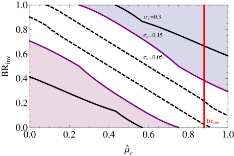
The sensitivity of this -based bound is expected to be equivalent to the sensitivity to in the PDF test in the Gaussian limit. Figure 4 shows the sensitivity band, as a function of for the PDF test, for several values of its error : the current one (); the combined error expected when both ATLAS and CMS accumulate enough data for a Higgs discovery per experiment over this year (), with the 95% CL excluded region shaded; and with a future error value down to . As expected, if is small this requires a large invisible width and a lower limit on can be set while, if is closer to 1, then only an upper limit on can be derived. For intermediate values of a “measurement” of would be possible. The plot shows that the error in the determination of the true value of (along the diagonal) is approximately . Note that for or , the corresponding values of themselves require smaller than for moderate values of to reach a discovery. Thus if a discovery is actually made in these cases, any corresponding will be simultaneously more accurately known than for the case.
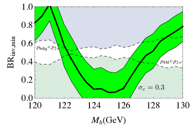
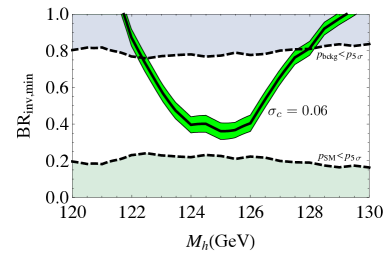
Finally, in Fig. 5 we translate the best-fit value obtained by combining the results of ATLAS, CMS and the Tevatron into a best-fit value for the (using ) as a function of .101010See also Ref. Low:2011kp for a recent analysis (on older data) with a similar reinterpretation of the data as in Fig. 5 (left). The left plot shows the current situation, with a best-fit for the interesting Higgs mass range GeV, which is in any case perfectly compatible with a zero value. The larger values of for other Higgs masses are also not statistically significant because they correspond to values of either or not particularly small (for reference, only above the lower dashed line, while only below the upper dashed line). This can change with higher energy/luminosity and the right plot shows a hypothetical future situation with nonzero Higgs invisible width after collection of more data (such that the current used in the left plot is reduced by a factor 5). Besides a hypothetical curve with the best value for , the plot also shows the regions of parameter space for which and are below , illustrating how such an analysis could claim indirect evidence for .
III Robustness of Global Fits to extract
In the previous section we have examined the prospects for bounding or discovering for the Higgs in BSM scenarios where new physics primarily couples to the dimension two scalar mass operator. In this section, we will examine how robust these conclusions are when a scalar resonance that has only approximately SM Higgs properties is involved in EWSB. First we will consider in Section III.1 the case of a minimal effective chiral EW Lagrangian with a non-linear realization of and a light scalar resonance. This scenario is most easily interpreted in composite Higgs scenarios and introduces parameters for the unknown coupling of a scalar resonance to the gauge and fermion fields of the SM, with the SM case corresponding to . (See Refs. Giudice:2007fh ; Contino:2010mh ; Grober:2010yv ). The obvious problem one faces in this case is how to determine if a universal reduction in signal yields is due to a nonzero or to a uniform reduction of the Higgs couplings involved in the search channels (i.e., ).
The robustness of global fits for in the presence of unknown higher dimensional operators is also important to determine. In Section II, when considering the effects of on the SM Higgs, it was assumed that all new light states are essentially not charged under , so that only Higgs decay (but not Higgs production) was affected, due to invisible decays to those states. When this assumption is relaxed, one can consider BSM scenarios in which, besides the light SM singlets leading to , heavier new states [charged under ] leave their trace in the low-energy effective theory through higher dimensional operators. In that case, it is important to examine the interplay of the effects of such higher dimensional operators on Higgs production and the effect of the light singlet states on in global fits. We study this question in Section III.4.
III.1 Global Fits to a Non-SM scalar resonance and extracting
In this section, we consider the more general case, consistent with the current data set, of a minimal effective chiral EW Lagrangian with a non-linear realization of and a light scalar resonance, denoted as . Such a theory includes the Goldstone bosons associated with the breaking of the weakly gauged (which is a subgroup of ) and the SM field content. This theory is the minimal effective theory of a light scalar degree of freedom that can have the experimentally supported pattern of MFV flavour breaking as in the SM, and respect custodial symmetry – , while the and are massive. (See Ref. Farina:2012ea for an analysis of the LHC data relaxing the assumption.) The Goldstone bosons are denoted by , where , and are grouped as
| (18) |
with and the Pauli matrices. The field transforms linearly under as where indicate the transformation on the left and right under and , respectively, while is the diagonal subgroup of , under which the scalar transforms as a singlet. The leading terms in the derivative expansion of such a theory are given by Giudice:2007fh ; Contino:2010mh ; Grober:2010yv ; Grinstein:2007iv
| (22) | |||||
Here we have neglected potential terms that are not relevant for the fits we will perform. Fitting the current data in such a theory has been recently explored in the literature Azatov:2012bz ; Espinosa:2012ir . Note that the SM Higgs is a special case of this theory, and corresponds to a linear completion ( becomes part of a linear multiplet) of this non-linear sigma model, with .
III.2 Imposing EWPD
It is useful to consider fitting to EWPD simultaneously with the global data to obtain a more constrained parameter space in this effective theory.111111In fact, we will find in subsequent sections that marginalization over multiple parameters in the three dimensional fit space including EWPD is required to obtain a residual distribution that is not flat. In EWPD analyses, the corrections to the gauge boson propagators in this effective Lagrangian can be expressed in terms of shifts of the oblique parameters S and T Holdom:1990tc ; Peskin:1991sw ; Altarelli:1990zd given by
| (23) |
These equations are approximate in that the numerical coefficient is determined from the logarithmic large dependence of given in Ref. Peskin:1991sw . Here we have introduced a Euclidean momentum cut-off scale , which approximately represents the mass of new states that are required to cut-off the growth in the longitudinal gauge boson scattering. In a full calculation, with all degrees of freedom, the cut-off scale will cancel. The degree to which this Euclidean cut-off properly captures the UV regularization of these integrals by new states not included in the effective theory is model dependent. We assume that the UV completion of the effective Lagrangian is such that directly treating this cut-off scale as a proxy for a heavy mass scale integrated out is valid, i.e. that further arbitrary parameters rescaling the cut-off scale terms need not be introduced. The cut-off scale is chosen to be for .
For EWPD we use the results of the collaboration Baak:2011ze for ,
| (24) |
and the correlation coefficient matrix is given by
| (28) |
We shift these results to having the input using the one-loop contribution of the SM Higgs field to S and T. This numerical shift is . There is a strong preference for in a global fit due to EWPD, i.e the SM mechanism of mass generation of the and is strongly preferred in minimal scenarios where EWPD can be directly interpreted to dictate the value of . When EWPD is imposed one has a bias in the fit space so that , but this should not be over-interpreted. This bias could in principle be a hint for the existence of other states in EWPD, but this possibility cannot be disentangled from cut-off scale effects without further experimental and theoretical input. We conservatively consider this bias to be simply a numerical artifact of our cut-off procedure.
Interestingly, EWPD offers a handle to disentangling the degeneracy between and the presence of : has a direct impact on EWPD, while the new singlet states (into which the Higgs can decay invisibly) can have no impact on EWPD. In any case, the possibility of such degeneracy implies that further cross-checks of would be needed to confirm an eventual indirect evidence coming from the global tests discussed in the last Section. Directly confirming such indirect evidence for is best accomplished in more traditional studies of experimental sensitivity to based on the kinematics of Higgs decay products. We discuss prospects for such a direct confirmation in Section IV.
III.3 Marginalizing/Fixing Parameters


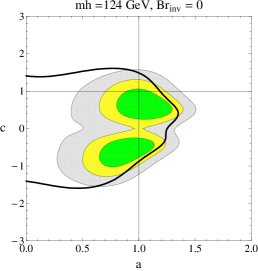
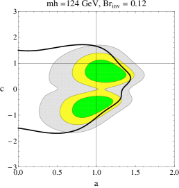

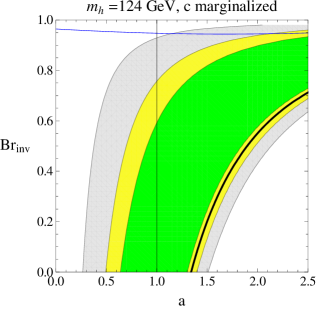
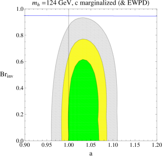
First, consider the case of fixing or marginalizing over one of the parameters 121212In the remainder of the paper we will always choose the value as we have shown that the fit results are not strongly dependent (considering current errors) on the chosen mass (when varied in the range ). to examine the robustness of our global fit results when is assumed, as in Ref. Espinosa:2012ir . Fits with various as an input value are shown in Fig. 6. We find that, when EWPD constraints are incorporated into the fit, the minimum of the is preferred for larger values of . This is easy to understand, as depends on the interference of fermion and gauge boson loops with an interference term . As the invisible width gets larger and the expected number of events in final states decreases, negative values of allow (by constructive interference) the number of events to be larger and more consistent with the data which show an excess in a number of subchannels. It is interesting that this is another example where the breaking of the approximate symmetry in the parameter space has a physical consequence. If (relative) excesses in the signal strengths of became statistically significant with a larger data set, coincident with common suppressions in the other discovery channels, such a pattern of deviations can be explained with a large and a negative in the effective theory, with constraints from EWPD.


Conversely, when EWPD are not used, the allowed parameter space is shifted to larger values of and as increases to (partially) cancel the suppression of events due to . More precisely, the lower plots shown in Fig. 6 have a simple scaling property corresponding to a dilatation from the origin in space, relating the spaces in plot to plot as
| (29) |
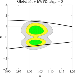
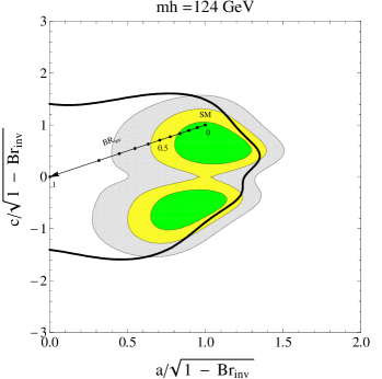
The constraints from EWPD on the fit space can be more easily understood by directly comparing the fit spaces as shown in Fig.7 (left). Similarly, the dilatation scaling of the best fit space is illustrated in Fig.7 (right) where we plot the fit space as a function of the scaling variables .
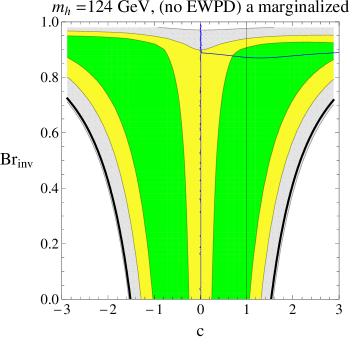
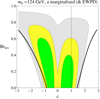
Now consider treating each one of the parameters as a nuisance parameter in turn. Doing so we can also examine the effects of an unknown parameter on the remaining fit space. For example, in marginalizing over we define a reduced function
| (30) |
where is given by the solution of . Then the allowed parameter space is defined through the CDF for a two parameter fit, and we obtain the results in Fig. 8. Marginalizing over the parameters and we find the results shown in Fig. 9 and Fig. 10 respectively which demonstrate the correlation between the allowed , and the allowed parameter space for the remaining unknown parameters. This correlation is due to the dilatation relationship shown in Eq. 29.
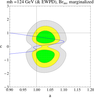
Finally one can marginalize two of the free parameters simultaneously in order to obtain the residual distribution to examine if the slight statistical preference for persists. In this case, one must impose EWPD to avoid a flat distribution in the remaining free parameter. We find the results shown in Fig. 11.


Of most interest is the result of marginalizing over free gauge and fermion couplings, while imposing EWPD. In this case, one finds that the global fit in this theory is now , with the CL limit , for a scalar mass of . Comparing this to the SMinv result of Section II, we see that an unknown can remove the slight preference for in the current global fits when the with is the global minimum. Conversely when the with is chosen, the slight preference for in the data set is not removed. Then the best fit is , with the CL limit . This result makes clear that performing such a two dimensional marginalization over is an important cross check to see if any evidence of is robustly preferred in a future data set.
III.4 Higher Dimensional Operators, , and the SM Higgs.
It is also of interest to consider the impact of possible BSM states on Higgs production and decay, when evidence for emerges from global fits. The exact impact of BSM states on Higgs phenomenology is model dependent. In this section, we consider the case where new states that are SM singlets lead to , and other new states, that are charged under , or at least a subgroup of the SM group, lead to higher dimensional operators. Our aim is to examine the degree to which conclusions about can be extracted from global fits in the context of unknown Wilson coefficients of the resulting higher dimensional operators.
Assuming that these BSM states do not source CP violation, the operators of interest for Higgs phenomenology (in global fits to ) are given by
| (31) | |||||
Note that are the weak hypercharge, gauge and gauge couplings and we are using the notation of Ref. Manohar:2006gz . The scale corresponds to the mass scale of the lightest new state that is integrated out. We are primarily interested in the effects on and as these are loop level processes in the SM, sensitive to BSM effects. As we expect loop level contributions to these operators from the BSM states, we rescale the Wilson coefficients as for and fit to combinations of .
Using the results of Ref. Manohar:2006gz , the effect of these operators are
| (32) |
Here and we have used , and . The imaginary part of the numerical coefficients above comes from including the quark loop correction (we use ) in normalizing the BSM effect to the SM amplitudes. Normalizing in this manner is done to reduce the SM dependence in the BSM correction when this rescaling is used in our fits, and a numerical value is used for . As in Ref. Manohar:2006gz , we have retained the two loop QCD correction to the SM matching of the operator in the limit in these numerical coefficients. Due to this choice, this correction cancels out (in the limit) of the overall coefficient of the BSM effects when multiplied by the numerical value of . This is a correction on the quoted numerical coefficient. Initial state radiation and vertex corrections to are expected to be common multiplicative factors for the operator in the limit, and as such are not incorporated in the numerical factors multiplying above. We will consider the parameter space where the SM is modified by these corrections and in this section, fitting to . The exact relationship between these parameters, if any, is model dependent and unknown. As such, we fit to the data assuming no relationship between the three parameters.131313See also Refs. Carmi:2012yp ; Giardino:2012ww ; Batell:2011pz , for example, for recent fits to BSM higher dimensional operator Wilson coefficients based on Higgs signal strength parameters.
The operators in also affect , where a different combination of the Wilson coefficients enters. This branching ratio is subdominant to the branching ratio. (Numerically the values are , and . However, recall that when looking for the Higgs, the decay has to be multiplied by .) We neglect these effects when fitting for the allowed parameter space. We also do not include the effects of these operators on as the SM contribution is tree level for these processes. Further, we also neglect effects due to higher dimensional operators possibly modifying the differential distributions of the Higgs decay products, indirectly affecting the through modifying the effective signal efficiency for specific kinematic cuts. Such effects are expected to be negligible compared to the current uncertainties. However, we do not neglect the rescaling effect on that is identified with the rescaling on in Eq. 32. We include this rescaling consistently, which has a non-negligible impact on all branching ratios through the modification of .

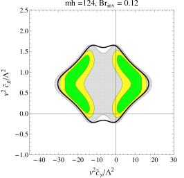


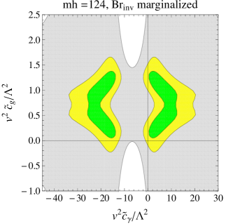
We show in Fig.12 the allowed parameter space when is fixed to prior values of , or . In Fig.13 the residual distribution for is shown when are marginalized over (left) and we also show the allowed parameter space when is marginalized over (right) subject to the prior constraint . These results show the significant impact of the higher dimensional operators, in scenarios consistent with the assumptions of this section, on attempts to extract from global fits to Higgs signal strength data.
Most notably, we find that the slight preference in the global distribution for is removed when marginalizing over such unknown BSM effects in the current data set. This offers further caution to over interpreting the slight preference in the global distribution for at this time. Although in Fig.12 the required Wilson coefficient to still obtain a good fit when is large, we find that even restricting to clearly perturbative couplings (), expected in many models, the preference for a is removed. This result is shown in Fig.13 (left).
IV Prospects for Direct confirmation of .
As stated above, there is a degeneracy between the case and the existence of a non-zero invisible decay. The former leaves the branching ratios unchanged due to a common suppression factor in the couplings, while all production channels are suppressed by the same common factor. On the other hand, in the simple case of leaving the SM couplings unchanged but allowing for an invisible width, the production channels are unchanged and the branching ratios are affected as in Eq. 3, leading to a common overall suppression of production times branching ratio compared to the SM. If a signal is seen with suppressed event rate with respect to the SM expectation the degeneracy between these two cases can only be removed by observing directly a non-vanishing invisible decay.
It has been shown that associated production with gauge bosons, weak boson fusion and associated production with top quarks allows one to discover a Higgs boson decaying invisibly, and to probe the invisible branching ratio. The typical signature is large missing transverse energy/momentum. Assuming an invisible branching ratio of 1, a Higgs boson with mass up to about 150 GeV can be discovered in Higgs radiation from a boson at fb-1 and TeV Choudhury:1993hv ; Frederiksen:1994me ; Godbole:2003it ; Davoudiasl:2004aj ; Zhu:2005hv ; Gagnon ; Meisel ; Warsinsky . At high luminosity this reach can be extended to GeV in associated production with a top quark pair Warsinsky ; Gunion:1993jf ; Kersevan:2002zj . Weak boson fusion allows for the discovery up to 480 GeV with 10 fb-1 integrated luminosity Warsinsky ; Eboli:2000ze ; Cavalli:2002vs ; Girolamo . Assuming SM production, invisible branching ratios as low as 25% can be probed in weak boson fusion for a 120 GeV Higgs boson at fb-1 and TeV at 95% CL Eboli:2000ze ; Cavalli:2002vs ; Girolamo . In associated production with a boson, branching ratios down to 45% can be probed Godbole:2003it ; Meisel ; Gagnon while associated Higgs production with a top quark pair probes invisible branching ratios down to 56% Kersevan:2002zj .
Recent papers have investigated the potential of a TeV collider in direct searches for an invisible Higgs boson Bai:2011wz ; Englert:2011us ; Englert:2011aa ; Djouadi:2012zc ; Frigerio:2012uc . The invisible branching ratio of a 125 GeV Higgs boson produced in weak boson fusion with SM strength can be constrained down to at TeV and fb-1 Bai:2011wz . Monojet searches from CMS based on 4.7 fb-1 cmsmonojet constrain down to 1.3 at 95% CL translating to the constrained value of the invisible branching ratio in case of SM couplings Djouadi:2012zc .
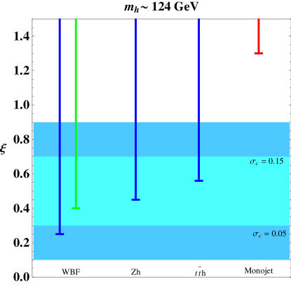
The claimed CL limits on expected for GeV from the direct searches discussed are summarized in Fig. 14. In this figure we also show for a direct comparison the sensitivity expected in the global test statistics we advocate for the end of this year, with and a future value when . One sees in this figure that the global test statistics are likely to offer a significantly improved reach for the existence of in the data set after the 2012 run. However, to claim a discovery of will require a combination of these global searches and direct kinematic searches, as we have demonstrated throughout Section III.
V Conclusions.
In this paper, we have systematically examined the potential of global fits to extract information on in the present and future signal strength data sets of a scalar resonance. We have focused on the case of a scalar resonance with mass , and have performed a global fit to the SM Higgs using the current signal strength data set, demonstrating that current global fits find the CL limit for . We have also illustrated how these results are statistically limited at this time and that any statistically significant conclusion on best fit values of will require more data. We have developed a new approach to globally combining signal strengths using global PDF’s to optimize searches for new states that couple to the SM through the ‘Higgs portal’. These promising results have lead us to examine the ability of global fits to resolve information on in the presence of unknown new physics effects simultaneously impacting the properties of the Higgs. Although disentangling these effects would require further experimental input, our results make clear the correlations expected between interpreting a global fit as providing evidence of and the sensitivity of such claims to other (unknown) new physics effects in the scenarios we have considered. Although the current signal strength data set we have considered in our numerical investigations only offers marginal evidence for a scalar resonance (and its properties) with GeV, the correlations with other new physics effects and the tests for evidence of we have explored are of continued interest as the data set evolves.
Appendix A Data Used
The data we have used in the global fits of this paper are summarized in the table below. Due to an apparent inconsistency in the ATLAS best fit signal strength plot for and the corresponding ATLAS limit plot (that is under investigation by ATLAS) we do not use the best fit signal strength value in the combined fit at this time. For the signal of CMS we assume a contamination due to Higgs production events so that the relevant signal rate is given by
| (33) |
Here is given by Higgs production. We do not use sub classes of events due to the lack of experimentally reported contaminations of these signal strengths due to other Higgs production processes. Simultaneously using a global best fit value for events (for example) while also using a best fit for a subclass of events, such as can result in a double counting of signal strengths that would incorrectly bias the fit. We avoid such double counting in our use of CMS and ATLAS data as the photon classes we use are exclusive, but note that double counting of this form is present in Ref. Giardino:2012ww , making it difficult to compare results. In particular, to avoid introducing such a bias is why we use the experimentally reported global ATLAS , as a complete set of subchannel di-photon signal strengths is not available (in contrast to CMS). This is also the reason that we do not simultaneously use constructed signal strengths and (from fermiophobic fermiophobic searches). These signal strengths are not independent mutually exclusive event classes, being derived from the same signal event data. Our approach to this issue is different than the approach of Ref. Giardino:2012ww .
| Channel [Exp] | ||
|---|---|---|
| Ref.TEVNPH:2012ab | ||
| Ref.TEVNPH:2012ab | ||
| Ref.moriond | ||
| Ref.ATLASdoc2011163 | ||
| Ref.moriond | ||
| Ref.ATLAS:2012ad | ||
| Ref.Chatrchyan:2012tx | ||
| Ref.Chatrchyan:2012tx | ||
| Ref.Chatrchyan:2012tx | ||
| Ref.Chatrchyan:2012tx | ||
| , Cat.4/BDT3, Refs.Chatrchyan:2012tw ; CMSdoc12001 | ||
| , Cat.3/BDT2, Refs.Chatrchyan:2012tw ; CMSdoc12001 | ||
| , Cat.2//BDT1, Refs.Chatrchyan:2012tw ; CMSdoc12001 | ||
| , Cat.1/BDT0, Refs.Chatrchyan:2012tw ; CMSdoc12001 | ||
| Refs.Chatrchyan:2012tw ; CMSdoc12001 |


For we use the public results presented at Moriond 2012 that split the signal events into four (multivariate boosted decision tree –BDT) classes that are not identical to the classes used for . See the relevant experimental papers for the detailed class definition in each case, but note that the event classes are exclusive (though correlated) and can be combined directly in our procedure. Once again correlation coefficients are neglected as they are not supplied, but the effect of pseudo-correlations have been examined in Ref. Espinosa:2012ir and the fit was found to be stable against randomly chosen correlations. Also we have found in Section II consistent results between two different approaches to the fit of signal-strength parameters: using the individual channels or the combined results. This indicates that neglected correlations do not bias the fit results outside the quoted errors.
Note that here we use a value of for the result for , unlike in Ref. Espinosa:2012ir , where we used the same value as for . This introduces a small interpolation error, but allows better agreement with global combined signal strengths reported by the Tevatron collaboration.
Acknowledgments
We thank A. Djouadi, R. Gonçalo, A. Juste, M. Martinez, M. Spira, W. Fisher, J. Huston, V. Sharma and J. Bendavid for helpful communication on related theory and data. This work has been partly supported by the European Commission under the contract ERC advanced grant 226371 MassTeV , the contract PITN-GA-2009-237920 UNILHC , and the contract MRTN-CT-2006-035863 ForcesUniverse , as well as by the Spanish Consolider Ingenio 2010 Programme CPAN (CSD2007-00042) and the Spanish Ministry MICNN under contract FPA2010-17747 and FPA2008-01430. MM is supported by the DFG SFB/TR9 Computational Particle Physics. Preprints: KA-TP-22-2012, SFB/CPP-12-32, CERN-PH-TH/2012-151.
References
- (1) L. Susskind, Phys. Rev. D 20 (1979) 2619.
- (2) S. Weinberg, Phys. Rev. D 19 (1979) 1277.
- (3) P. Sikivie et al. Nucl. Phys. B 173 (1980) 189.
- (4) M. A. Shifman et al. Sov. J. Nucl. Phys. 30, 711 (1979) [Yad. Fiz. 30, 1368 (1979)].
- (5) A. I. Vainshtein et al. Sov. Phys. Usp. 23, 429 (1980) [Usp. Fiz. Nauk 131, 537 (1980)].
- (6) ATLAS-CONF-2012-019.
- (7) CMS-HIG-12-008.
- (8) D. Carmi, A. Falkowski, E. Kuflik and T. Volansky, [hep-ph/1202.3144].
- (9) A. Azatov, R. Contino and J. Galloway, JHEP 1204 (2012) 127 [hep-ph/1202.3415].
- (10) J. R. Espinosa, C. Grojean, M. Muhlleitner and M. Trott, [hep-ph/1202.3697].
- (11) R. Lafaye et al. JHEP 0908, 009 (2009) [hep-ph/0904.3866].
- (12) C. Englert et al. Phys. Lett. B 707, 512 (2012) [hep-ph/1112.3007].
- (13) M. Klute et al. [hep-ph/1205.2699].
- (14) R. Schabinger and J. D. Wells, Phys. Rev. D 72, 093007 (2005) [hep-ph/0509209].
- (15) B. Patt and F. Wilczek, hep-ph/0605188.
- (16) S. Chang et al. Ann. Rev. Nucl. Part. Sci. 58, 75 (2008) [hep-ph/0801.4554].
- (17) J. March-Russell et al. JHEP 0807, 058 (2008) [hep-ph/0801.3440].
- (18) J. R. Espinosa and M. Quiros, Phys. Rev. D 76, 076004 (2007) [hep-ph/0701145].
- (19) M. Pospelov and A. Ritz, Phys. Rev. D 84, 113001 (2011) [hep-ph/1109.4872].
- (20) S. Dittmaier et al. [LHC Higgs Cross Section Working Group Collaboration], [hep-ph/1101.0593].
- (21) P. P. Giardino, K. Kannike, M. Raidal and A. Strumia, [hep-ph/1203.4254].
- (22) M. Pieri, Talk on behalf of CMS and ATLAS, CERN, 24 May, 2012
- (23) I. Low, P. Schwaller, G. Shaughnessy and C. E. M. Wagner, Phys. Rev. D 85, 015009 (2012) [hep-ph/1110.4405].
- (24) TEVNPH and CDF and D0 Collaborations, [hep-ex/1203.3774].
- (25) G. F. Giudice, C. Grojean, A. Pomarol and R. Rattazzi, JHEP 0706, 045 (2007) [hep-ph/0703164].
- (26) R. Contino et al JHEP 1005, 089 (2010) [hep-ph/1002.1011].
- (27) R. Grober and M. Muhlleitner, JHEP 1106, 020 (2011) [hep-ph/1012.1562].
- (28) M. Farina, C. Grojean and E. Salvioni, [hep-ph/1205.0011].
- (29) B. Grinstein and M. Trott, Phys. Rev. D 76, 073002 (2007) [hep-ph/0704.1505].
- (30) B. Holdom and J. Terning, Phys. Lett. B 247 (1990) 88. M. E. Peskin and T. Takeuchi, Phys. Rev. Lett. 65 (1990) 964. M. Golden and L. Randall, Nucl. Phys. B 361 (1991) 3.
- (31) M. E. Peskin and T. Takeuchi, Phys. Rev. D 46 (1992) 381.
- (32) G. Altarelli and R. Barbieri, Phys. Lett. B 253 (1991) 161. G. Altarelli, R. Barbieri and S. Jadach, Nucl. Phys. B 369 (1992) 3 [Erratum-ibid. B 376 (1992) 444].
- (33) M. Baak et al. [hep-ph/1107.0975].
- (34) A. V. Manohar and M. B. Wise, Phys. Lett. B 636, 107 (2006) [hep-ph/0601212].
- (35) B. Batell, S. Gori and L. -T. Wang, [hep-ph/1112.5180].
- (36) D. Choudhury and D. P. Roy, Phys. Lett. B 322 (1994) 368 [hep-ph/9312347].
- (37) S. G. Frederiksen, N. Johnson, G. L. Kane and J. Reid, Phys. Rev. D 50 (1994) 4244.
- (38) R. M. Godbole et al Phys. Lett. B 571 (2003) 184 [hep-ph/0304137].
- (39) H. Davoudiasl, T. Han and H. E. Logan, Phys. Rev. D 71 (2005) 115007 [hep-ph/0412269].
- (40) S. -h. Zhu, Eur. Phys. J. C 47 (2006) 833 [hep-ph/0512055].
- (41) P. Gagnon, ATL-PHYS-PUB-2005-011.
- (42) F. Meisel et al., ATL-PHYS-PUB-2006-009.
- (43) M. Warsinsky, J. Phys. Conf. Ser. 110 (2008) 072046; M. Heldmann, APP. B 38 (2007) 787.
- (44) J. F. Gunion, Phys. Rev. Lett. 72 (1994) 199 [hep-ph/9309216].
- (45) B. P. Kersevan, M. Malawski and E. Richter-Was, Eur. Phys. J. C 29 (2003) 541 [hep-ph/0207014].
- (46) O. J. P. Eboli and D. Zeppenfeld, Phys. Lett. B 495 (2000) 147 [hep-ph/0009158].
- (47) D. Cavalli et al., hep-ph/0203056.
- (48) B. Di Girolamo, L. Neukermans, ATL-PHYS-PUB-2003-006.
- (49) C. Englert, J. Jaeckel, E. Re and M. Spannowsky, Phys. Rev. D 85 (2012) 035008 [hep-ph/1111.1719].
- (50) Y. Bai, P. Draper and J. Shelton, [hep-ph/1112.4496].
- (51) A. Djouadi, A. Falkowski, Y. Mambrini and J. Quevillon, [hep-ph/1205.3169].
- (52) M. Frigerio, A. Pomarol, F. Riva and A. Urbano, JHEP 1207, 015 (2012) [arXiv:1204.2808 [hep-ph]].
- (53) CMS-PAS-EXO-11-059, and the Winter 2012 update.
- (54) ATLAS-CONF-2012-013.
- (55) Rencontres de Moriond 2012, http://moriond.in2p3.fr/
- (56) ATLAS-CONF-2011-163.
- (57) G. Aad et al. [ATLAS Collaboration], Phys. Rev. Lett. 108, 111803 (2012) [hep-ex/1202.1414].
- (58) S. Chatrchyan et al. [CMS Collaboration], Phys. Lett. B 710, 26 (2012) [hep-ex/1202.1488].
- (59) S. Chatrchyan et al. [CMS Collaboration], [hep-ex/1202.1487].
- (60) CMS PAS HIG-12-001.