DIRECT CP VIOLATION IN D-MESON DECAYS

Recently, the LHCb and CDF collaborations reported a surprisingly large difference between the direct CP asymmetries, $\Delta{\cal A}_{CP}$, in the $D^{0}\to K^{+}K^{-}$ and $D^{0}\to\pi^{+}\pi^{-}$ decay modes. An interesting question is whether this measurement can be explained within the standard model. In this review, I would like to convey two messages: First, large penguin contractions can plausibly account for this measurement and lead to a consistent picture, also explaining the difference between the decay rates of the two modes. Second, “new physics” contributions are by no means excluded; viable models exist and can possibly be tested.

1 Introduction

The $D^{0}\to K^{+}K^{-}$ and $D^{0}\to\pi^{+}\pi^{-}$ decays are induced by the weak interaction via an exchange of a virtual $W$ boson and suppressed by a single power of the Cabibbo angle. Direct $CP$ violation in singly Cabibbo-suppressed (SCS) $D$-meson decays is sensitive to contributions of new physics in the up-quark sector, since it is expected to be small in the standard model: the penguin amplitudes necessary for interference are down by a loop factor and small Cabibbo-Kobayashi-Maskawa (CKM) matrix elements, and there is no heavy virtual top quark which could provide substantial breaking of the Glashow-Iliopoulos-Maiani (GIM) mechanism. Naively, one would thus expect effects of order $\mathcal{O}([V_{cb}V_{ub}/V_{cs}V_{us}]\alpha_{s}/\pi)\sim 0.01\%$.

We define the amplitudes for final state $f$ as

$$\begin{split}A_{f}&\equiv A(D\to f)=A^{T}_{f}\big{[}1+r_{f}e^{i(\delta_{f}-\phi_{f})}\big{]},\\ \overline{A}_{f}&\equiv A(\bar{D}\to f)=A^{T}_{f}\big{[}1+r_{f}e^{i(\delta_{f}+\phi_{f})}\big{]}\,.\end{split}$$ (1)

Here $A^{T}_{f}$ is the dominant tree amplitude and $r_{f}$ the relative magnitude of the subleading amplitude, carrying the weak phase $\phi_{f}$ and the strong phase $\delta_{f}$. We can now define the direct $CP$ asymmetry as

$$\begin{split}{\cal A}_{f}^{\rm dir}\equiv{|A_{f}|^{2}-|\bar{A}_{f}|^{2}\over|A_{f}|^{2}+|\bar{A}_{f}|^{2}}=2r_{f}\sin\gamma\sin\delta_{f}\,,\end{split}$$ (2)

where the last equality holds up to corrections of $\mathcal{O}(r_{f}^{2})$. LHCb and CDF measure a time-integrated $CP$ asymmetry. The approximately universal contribution of indirect $CP$ violation cancels to good approximation in the difference

$$\begin{split}\Delta{\cal A}_{CP}={\cal A}_{CP}(D\to K^{+}K^{-})-{\cal A}_{CP}(D\to\pi^{+}\pi^{-})\,.\end{split}$$ (3)

The measurements of LHCb, $\Delta{\cal A}_{CP}=(-0.82\pm 0.21\pm 0.11)\%$ $\!{}^{{\bf?}}$, CDF, $\Delta{\cal A}_{CP}=(-0.62\pm 0.21\pm 0.10)\%$ $\!{}^{{\bf?}}$, and inclusion of the indirect $CP$ asymmetry $A_{\Gamma}$ $\!{}^{{\bf?},{\bf?}}$, lead to the new world average (including the Babar $\!{}^{{\bf?}}$, Belle $\!{}^{{\bf?}}$, and CDF $\!{}^{{\bf?}}$ measurements) $\Delta{\cal A}_{CP}=(-0.67\pm 0.16)\%$ $\!{}^{{\bf?}}$. In the following, we will try to answer three questions: Can this measurement be accounted for by the standard model? Can it be new physics? Can we distinguish the two possibilities?

2 Setting the stage

As a first step, we take the size of the tree amplitudes $A^{T}$ from data and then relate the tree amplitudes to the penguin amplitudes $A^{P}$ to estimate the size of the latter $\!{}^{{\bf?}}$. The starting point of our analysis is the weak effective Hamiltonian

$$\begin{split}H_{\rm eff}^{\rm SCS}=\frac{G_{F}}{\sqrt{2}}&\left\{\left(V_{cs}V_{us}^{*}-V_{cd}V_{ud}^{*}\right)\sum_{i=1,2}C_{i}\left(Q_{i}^{\bar{s}s}-Q_{i}^{\bar{d}d}\right)/2\right.\\ &\left.-V_{cb}V_{ub}^{*}\,\left[\sum_{i=1,2}C_{i}\left(Q_{i}^{\bar{s}s}+Q_{i}^{\bar{d}d}\right)/2+\sum_{i=3}^{6}C_{i}Q_{i}+C_{8g}Q_{8g}\,\,\right]\right\}+{\rm h.c.}\,.\end{split}$$ (4)

The Wilson coefficients of the tree operators $Q_{1}^{\bar{p}p^{\prime}}=(\bar{p}u)_{V-A}\otimes(\bar{c}p^{\prime})_{V-A}$, $Q_{2}^{\bar{p}p^{\prime}}=(\bar{p}_{\alpha}u_{\beta})_{V-A}\otimes\\ (\bar{c}_{\beta}p^{\prime}_{\alpha})_{V-A}$, the penguin operators $Q_{3\ldots 6}$, and the chromomagnetic operator $Q_{8g}$, can be calculated in perturbation theory. The hadronic matrix elements are harder to compute; we will estimate their size using experimental data. They receive leading power contributions and power corrections in $1/m_{c}$, which are expected to be large.

A leading power estimation, using naive factorization and $\mathcal{O}(\alpha_{s})$ corrections, yields for the ratio $r_{f}^{\text{LP}}\equiv|A^{P}_{f}(\text{leading power})/A^{T}_{f}(\text{experiment})|$: $r_{K^{+}K^{-}}^{\text{LP}}\approx(0.01-0.02)\%$, $r_{\pi^{+}\pi^{-}}^{\text{LP}}\approx(0.015-0.028)\%$. This is consistent with, yet slightly larger than the naive scaling estimate. We expect the signs of ${\cal A}_{K^{+}K^{-}}^{\text{dir}}$ and ${\cal A}_{\pi^{+}\pi^{-}}^{\text{dir}}$ to be opposite, if $SU(3)$ breaking is not too large; so for $\phi_{f}=\gamma\approx 67^{\circ}$ and $\mathcal{O}(1)$ strong phases we obtain $\Delta{\cal A}_{CP}(\text{leading power})=\mathcal{O}(0.1\%)$, an order of magnitude smaller than the measurement.

However, we know from $SU(3)$ fits $\!{}^{{\bf?},{\bf?},{\bf?},{\bf?},{\bf?}}$ that power corrections can be large. To be specific, we look at insertions of the penguin operators $Q_{4}$, $Q_{6}$ into power-suppressed annihilation amplitudes. The associated penguin contractions of $Q_{1}$ cancel the scale and scheme dependence. Estimating their size using the loop functions $G$, defined in $\!{}^{{\bf?}}$, and using naive $N_{c}$ counting to relate the penguin to the tree amplitudes, we arrive at $r_{f,1}^{\text{PC}}\approx(0.04-0.08)\%$, $r_{f,2}^{\text{PC}}\approx(0.03-0.04)\%$, where $r_{f,i}^{\text{PC}}\equiv|A^{P}_{f}(\text{power correction})/A^{T}_{f}(\text{experiment})|$ and the subscripts $1,2$ correspond to the insertions of $Q_{4}$, $Q_{6}$, respectively. Again assuming $\mathcal{O}(1)$ strong phases, this leads to $\Delta{\cal A}_{CP}(r_{f,1})=\mathcal{O}(0.3\%)$ and $\Delta{\cal A}_{CP}(r_{f,2})=\mathcal{O}(0.2\%)$ for the two insertions. Thus, a standard model explanation seems plausible.

Of course, the extraction of the annihilation amplitudes from data, neglected contributions to the annihilation amplitudes, $N_{c}$ counting, the modeling of the penguin contraction amplitudes, and the neglected additional penguin contractions lead to an uncertainty of a factor of a few. So, can we trust the estimate?

3 A consistent picture

Another interesting observation is the large difference of SCS branching ratios, $\text{Br}(D^{0}\to K^{+}K^{-})\approx 2.8\times\text{Br}(D^{0}\to\pi^{+}\pi^{-})$. It implies that the ratio of amplitudes (normalized to phase space) is $A(D^{0}\to K^{+}K^{-})\approx 1.8\times A(D^{0}\to\pi^{+}\pi^{-})$, whereas they would be equal in the $SU(3)$ limit. This has often been interpreted as a sign of large $SU(3)$ breaking. On the other hand, the ratio of the Cabibbo-favored (CF) to the doubly Cabibbo-suppressed (DCS) amplitude is $A(D^{0}\to K^{-}\pi^{+})\approx 1.15\times A(D^{0}\to K^{+}\pi^{-})$, after accounting for CKM factors, in accordance with nominal $SU(3)$ breaking of $\mathcal{O}(20\%)$.

A glance at the effective Hamiltonian (4) shows that the combination $P$ of penguin contractions of $Q_{1,2}^{\bar{s}s}$ and $Q_{1,2}^{\bar{d}d}$ proportional to $V_{cb}V_{ub}^{*}$ is $U$-spin invariant, while $P_{\text{break}}$, the combination contributing to the tree amplitude vanishes in the $U$-spin limit. $P_{\text{break}}$ contributes with opposite sign to the two SCS decay rates, and $P$ gives rise to a nonvanishing $\Delta{\cal A}_{CP}$. Guided by the considerations exposed in Section 2, we perform a $U$-spin decomposition of the amplitudes to all four (CF, SCS, DCS) decays, and fit these amplitudes to the data (branching ratios and $CP$ asymmetries) under the additional assumption that penguin contractions are large, of order $\mathcal{O}(1/\epsilon)$, where $\epsilon\ll 1$.

Our main point is $\!{}^{{\bf?}}$ that under the assumption of nominal $U$-spin breaking, a broken penguin $P_{\rm break}$ which explains the difference of the $D^{0}\to K^{+}K^{-}$ and $D^{0}\to\pi^{+}\pi^{-}$ decay rates implies a $\Delta U=0$ penguin $P$ that naturally yields the observed $\Delta{\mathcal{A}}_{CP}$. The scaling $P_{\rm break}\sim\epsilon_{U}P$ together with our fit result $P_{\rm break}\sim T/2$ (see Fig. 1) yields the estimate

$$r_{\pi^{+}\pi^{-},K^{+}K^{-}}\simeq\left|\frac{V_{cb}V_{ub}}{V_{cs}V_{us}}\right|\cdot\left|\frac{P}{T\pm P_{\rm break}}\right|\sim\frac{|V_{cb}V_{ub}|}{|V_{cs}V_{us}|}\frac{1}{2\,\epsilon_{U}}\sim 0.2\%,$$ (5)

for $\epsilon_{U}\sim 0.2$. This is consistent with the measured $\Delta{\mathcal{A}}_{CP}$ for $\mathcal{O}(1)$ strong phases. Some results of our fit are shown in Figure 1.

                             

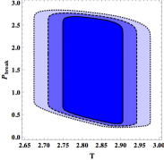
Figure 1: The results of our fit. Solid, dashed, and dotted lines denote one-, two-, and three-sigma contours, respectively. Left panel: A fit to the branching ratios only yields $P_{\text{break}}\equiv\epsilon_{sd}^{(1)}P\sim T$, assuming nominal $U$-spin breaking. $T$ is the tree amplitude. The lower bound of $P/T_{\text{avg}}$ in the middle panel is directly related to the large difference of decay rates for the SCS modes. ($T_{\text{avg}}$ is the average value of $T$ from the fit). It translates into the upper bound on $\Delta{\cal A}_{CP}$ – the fit results can naturally accommodate the measured value (right panel).

By the same reasoning, exchanging the spectator quark we expect direct $CP$ asymmetries of the same order ($\approx 0.5\%$) in the decay modes $D^{+}\to K^{+}\overline{K^{0}}$, $D_{s}^{+}\to\pi^{+}K^{0}$.

4 Can it be new physics?

Whereas a standard-model explanation seems plausible, it is not excluded that new physics contributes partly to $\Delta{\cal A}_{CP}$. Any new-physics explanation has to respect constraints from other observables like $D$- and $K$-meson mixing, or direct searches, but substantial contributions are still possible $\!{}^{{\bf?},{\bf?}}$. Can we discriminate them from the standard-model contributions?

Models of new physics that have $\Delta I=3/2$ contributions could be separated from the standard-model background (an example would be a scalar color-singlet weak doublet $\!{}^{{\bf?}}$). To see this, note that the standard-model tree operators have both $\Delta I=1/2$ and $\Delta I=3/2$ contributions, while the standard-model penguin operators are pure $\Delta I=1/2$ (apart from neglegible electroweak contributions). For instance, the $I=2$ final state in $D^{+}\to\pi^{+}\pi^{0}$ cannot be reached by standard-model penguin operators, so any observed direct $CP$ asymmetry in this decay would be a clear signal of new physics. More sophisticated isospin sum rules can be constructed $\!{}^{{\bf?}}$.

If new physics induces only $\Delta I=1/2$ transitions, it seems necessary to build explicit models and look for their collider signatures. The most plausible models include chirally enhanced chromomagnetic penguin operators $\!{}^{{\bf?},{\bf?}}$.

5 Conclusion

Large penguin contractions in the standard model can naturally explain both the large difference of decay rates in the $D^{0}\to K^{+}K^{-}$ and $D^{0}\to\pi^{+}\pi^{-}$ modes and the observed $\Delta{\cal A}_{CP}$. However, new-physics contributions are not excluded. Viable models exist and can possibly tested.

References

References

- [1] R. Aaij et al. [LHCb Collaboration], arXiv:1112.0938 [hep-ex].
- [2] A. Di Canto, talk at XXVI Rencontres de Physique de la Vallee d’Aoste Feb 26th-Mar 3rd 2012, La Thuile, Italy; CDF Note 10784.
- [3] B. Aubert et al. [BaBar Collaboration], Phys. Rev. Lett. 100, 061803 (2008)
- [4] M. Staric et al. [Belle Collaboration], Phys. Lett. B 670, 190 (2008)
- [5] B. Aubert et al. [BABAR Collaboration], Phys. Rev. D 78, 011105 (2008)
- [6] M. Staric et al. [Belle Collaboration], Phys. Rev. Lett. 98, 211803 (2007)
- [7] T. Aaltonen et al. [CDF Collaboration], Phys. Rev. D 85, 012009 (2012)
- [8] J. Brod, A. L. Kagan and J. Zupan, arXiv:1111.5000 [hep-ph].
- [9] H. Y. Cheng and C. W. Chiang, Phys. Rev. D 81 (2010) 074021 [arXiv:1001.0987 [hep-ph]].
- [10] D. Pirtskhalava and P. Uttayarat, arXiv:1112.5451 [hep-ph].
- [11] H. Y. Cheng and C. W. Chiang, arXiv:1201.0785 [hep-ph].
- [12] B. Bhattacharya, M. Gronau and J. L. Rosner, arXiv:1201.2351 [hep-ph].
- [13] T. Feldmann, S. Nandi and A. Soni, arXiv:1202.3795 [hep-ph].
- [14] J. Brod, Y. Grossman, A. L. Kagan and J. Zupan, arXiv:1203.6659 [hep-ph].
- [15] M. Beneke, G. Buchalla, M. Neubert and C. T. Sachrajda, Nucl. Phys. B 606, 245 (2001)
- [16] G. Isidori, J. F. Kamenik, Z. Ligeti and G. Perez, Phys. Lett. B 711, 46 (2012)
- [17] W. Altmannshofer, R. Primulando, C. -T. Yu and F. Yu, JHEP 1204, 049 (2012)
- [18] Y. Hochberg and Y. Nir, arXiv:1112.5268 [hep-ph].
- [19] Y. Grossman, A. L. Kagan and J. Zupan, arXiv:1204.3557 [hep-ph].
- [20] Y. Grossman, A. L. Kagan and Y. Nir, Phys. Rev. D 75, 036008 (2007)
- [21] G. F. Giudice, G. Isidori and P. Paradisi, JHEP 1204, 060 (2012)