Excess Wings in Broadband Dielectric Spectroscopy

Abstract

Analysis of excess wings in broadband dielectric spectroscopy data of glass forming materials is found to provide evidence for anomalous time evolutions and fractional semigroups. Solutions of fractional evolution equations in frequency space are used to fit dielectric spectroscopy data of glass forming materials with a range between 4 and 10 decades in frequency. We show that with only three parameters (two relaxation times plus one exponent) excellent fits can be obtained for 5-methyl-2-hexanol and for methyl-m-toluate over up to 7 decades. The traditional Havriliak-Negami fit with three parameters (two exponents and one relaxation time) fits only 4-5 decades. Using a second exponent, as in Havriliak-Negami fits, the $\alpha$-peak and the excess wing can be modeled perfectly with our theory for up to 10 decades for all materials at all temperatures considered here. Traditionally this can only be accomplished by combining two Havriliak-Negami functions with 6 parameters. The temperature dependent relaxation times are fitted with the Vogel-Tammann-Fulcher relation which provides the corresponding Vogel-Fulcher temperatures. The relaxation times turn out to obey almost perfectly the Vogel-Tammann-Fulcher law. Finally we report new and computable expressions of time dependent relaxation functions corresponding to the frequency dependent dielectric susceptibilities.

I Introduction

Many physical properties of glass forming liquids (e.g. their viscosity) vary dramatically (often over 15 or more decades) within a narrow temperature interval LSBL000 . This phenomenon is the glass transition. The change of physical properties during the glass transition has not yet been fully understood and remains a subject of intense investigations Lunkenheimer96 ; Corezzi2 ; Feldman2 ; Corezzi ; Kalinovskaya ; LoidlPC ; LoidlGlycerol ; Feldman100 ; Feldman50 ; RoskildeNature2008 ; RoskildeChemPhys2009 .

In this work we study the glass transition by observing the dielectric susceptibility. The dielectric susceptibility quantifies the response of permanent and induced dipoles to an applied frequency dependent electric field. The dielectric loss (resp. imaginary part of the complex dielectric susceptibility) typically shows a temperature dependent maximum, the $\alpha$-peak, at low frequencies. It is followed at higher frequencies by a so called excess wing KS003 . This excess wing has not yet been understood nor has it been described by any model with less then 4 fit parameters KS003 . Existing theories, such as the mode coupling theory (see mode_coupling_gotze98 ; mode_coupling_Reichman05 and references therein), do not allow to fit the excess wing. Traditional phenomenological fits of the excess wing employ a superposition of two Havriliak-Negami functions HavriliakNegami66 ; Corezzi ; KS003 , and they need 7 fit parameters to fit a range of 10 decades.

The aim of this work is to provide fit functions for excess wings with only three (four) parameters (one (two) exponent(s) and two relaxation times) obtained from the previously introduced method of fractional time evolution hil02c ; HilferFracRel2003 , and to apply them to experimental data exhibiting a clear excess wing on a frequency range as broad as possible. Our fitting functions need only 3 (model A) or 4 (model B) parameters, which is a significant improvement compared to 6 parameters for the superposition of the Havriliak-Negami and Cole-Cole expression presently used. We study the glass forming materials 5-methyl-2-hexanol Kalinovskaya , glycerol LoidlGlycerol and methyl-m-toluate RoskildeChemPhys2009 .

II Classical relaxation models

The Debye relaxation model describes the electric relaxation of dipoles after switching an applied electric field fro49 . The normalized relaxation function $f(t)$, which corresponds to the polarization, obeys the Debye law

$$\left(\tau\frac{\mbox{${\rm d}$}{}}{\mbox{${\rm d}$}{}t}+1\right)f(t) = 0,$$ (1)

with the relaxation time $\tau$ and initial condition $f(0)=1$. The response function, i.e. the dynamical dielectric susceptibility, $\chi$ is related to the relaxation function via hil02c

$$\chi(t)=-\frac{\mbox{${\rm d}$}{}}{\mbox{${\rm d}$}{}t}f(t).$$ (2)

In the following discussions we focus on Laplace transformed quantities. We use the Laplace transformation of $f(t)$

$$\mbox{${\mathscr{L}}$}{}\{f(t)\}(u)=\int_{0}^{\infty}e^{-ut}f(t)\ \mbox{${\rm d}$}{}t,$$ (3)

where $u=i\nu$ and $\nu$ is the frequency. Rewriting equation (2) in frequency space and utilizing $f(0)=1$ leads to

$$\hat{\chi}(u) = \mbox{${\mathscr{L}}$}{}\{\chi(t)\}(u)$$ (4)

$$= 1-u\mbox{${\mathscr{L}}$}{}\{f(t)\}(u)$$

$$= \frac{1}{1+u\tau},$$

the well known Debye susceptibility.

In experiments one measures not the normalized quantity $\hat{\chi}(u)$, but instead

$$\varepsilon(u)=(\varepsilon_{0}-\varepsilon_{\infty})\hat{\chi}(u)+\varepsilon_{\infty},$$ (5)

where $\varepsilon_{0}$ and $\varepsilon_{\infty}$ are the dynamical susceptibilities at low, respectively high frequencies.

The Debye model is not able to describe the experimental data well, because experimental relaxation peaks are broader and asymmetric. For this reason other fitting functions were proposed like the Cole-Cole cole-cole42 , Cole-Davidson cole-davidson51 and Havriliak-Negami HavriliakNegami66 expressions, whose normalized forms have typically 2 or 3 parameters (see table 1). They were introduced purely phenomenologically to fit the data. This can be considered as a drawback. These functions with three parameters are able to fit the data over a range of at most $5$ decades (Havriliak-Negami). Several copies are commonly superposed to fit a broader range, e.g. Havriliak-Negami plus Cole-Cole, which would result in 6 fit parameters.

Table 1: List of traditional fit functions for dielectric spectroscopy data of glass forming materials.

$\hat{\chi}(u)$ number of parameters Cole-Cole $1/(1+(u\tau)^{\alpha})$ 2 Cole-Davidson $1/(1+u\tau)^{\alpha}$ 2 Havriliak-Negami $1/(1+(u\tau)^{\alpha})^{\gamma}$ 3

III Fractional relaxation models

In this work we use a generalized form of the Debye relaxation model in equation (1). It is based on the theory of fractional time evolutions for macroscopic states of many body systems first proposed in equation (5.5) in hil93e and subsequently elaborated in hil95c ; hil95e ; hil95f ; hil98e ; hil00a ; hil02a ; hil02c ; hil03d ; hil03e ; hil07e ; hil11b . As discussed in hil02a ; hil02c composite fractional time evolutions are expected near the glass transition. Such time evolutions give rise to generalized Debye laws of the form of model A:

$$\left(\tau_{1}\mbox{${\rm D}$}{}+\tau_{2}^{\alpha}\mbox{${\rm D}$}{}^{\alpha}+1\right)f(t)=0$$ (6)

or model B:

$$\left(\tau_{1}\mbox{${\rm D}$}{}+\tau_{1}^{\alpha_{1}}\mbox{${\rm D}$}{}^{\alpha_{1}}+\tau_{2}^{\alpha_{2}}\mbox{${\rm D}$}{}^{\alpha_{2}}+1\right)f(t)=0,$$ (7)

where the parameters obey $0<\alpha,\alpha_{1},\alpha_{2}<1$, $\alpha_{1}>\alpha_{2}$ and the relaxation times $\tau_{1},\tau_{2}>0$ are positive. Here the symbols $\tau_{1}\mbox{${\rm D}$}{}+\tau_{2}^{\alpha}\mbox{${\rm D}$}{}^{\alpha}$, respectively $\tau_{1}\mbox{${\rm D}$}{}+\tau_{1}^{\alpha_{1}}\mbox{${\rm D}$}{}^{\alpha_{1}}+\tau_{2}^{\alpha_{2}}\mbox{${\rm D}$}{}^{\alpha_{2}}$ are the infinitesimal generators of composite fractional semigroups with $\mbox{${\rm D}$}{}^{\alpha}$ being a generalized fractional Riemann-Liouville derivative of order $\alpha$ and almost any type hil00a ; hil09d . If $\mbox{${\rm D}$}{}^{\nu}$ represents a classical fractional Riemann-Liouville derivative of order $\nu$ then its definition reads (with $\nu\in\mathbb{R}^{+}$)

$$\mbox{${\rm D}$}{}^{\nu}f(t) = \mbox{${\rm D}$}{}^{\lceil\nu\rceil}\mbox{${\rm I}$}{}^{\mu}f(t)$$ (8)

$$= \frac{1}{\Gamma(\mu)}\mbox{${\rm D}$}{}^{\lceil\nu\rceil}\int\limits_{0}^{t}(t-\xi)^{\mu-1}f(\xi)\ \mbox{${\rm d}$}{}\xi,$$

$$\mu+\nu=\lceil\nu\rceil,\quad t>0,$$

where $\lceil\nu\rceil$ is the smallest integer greater or equal $\nu$, $\Gamma$ the gamma function and $\mbox{${\rm D}$}{}^{\lceil\nu\rceil}=\mbox{${\rm d}$}{}^{\lceil\nu\rceil}/\mbox{${\rm d}$}{}t^{\lceil\nu\rceil}$.

The Laplace transform of the fractional Riemann-Liouville derivative is MillerRoss

$$\mbox{${\mathscr{L}}$}{}\{\mbox{${\rm D}$}{}^{\nu}f(t)\}(u) = u^{\nu}\mbox{${\mathscr{L}}$}{}\{f(t)\}(u)$$ (10)

$$-\sum_{k=1}^{\lceil\nu\rceil}u^{k-1}\left.\mbox{${\rm D}$}{}^{\nu-k}f(t)\right|_{t=0}.$$

With these definitions the Laplace transformation of equations (6) and (7) gives with relation (2) the normalized dielectric susceptibilities of model A

$$\hat{\chi}_{\rm A}(u)=\frac{\displaystyle{1+\tau_{2}^{\alpha}u^{\alpha}}}{\displaystyle{\tau_{1}u+\tau_{2}^{\alpha}u^{\alpha}+1}}$$ (11)

and model B

$$\hat{\chi}_{\rm B}(u)=\frac{\displaystyle{1+\tau_{1}^{\alpha_{1}}u^{\alpha_{1}}+\tau_{2}^{\alpha_{2}}u^{\alpha_{2}}}}{\displaystyle{\tau_{1}u+\tau_{1}^{\alpha_{1}}u^{\alpha_{1}}+\tau_{2}^{\alpha_{2}}u^{\alpha_{2}}+1}}.$$ (12)

These results apply also for other types of generalized Riemann-Liouville fractional derivatives introduced in hil02a ; hil02c .

The functions from equations (11) and (12) are used to fit the dielectric spectroscopy data of 5-methyl-2-hexanol, glycerol and methyl-m-toluate. Real and imaginary part are fitted simultaneously with the parameters $\alpha$, $\alpha_{1}$, $\alpha_{2}$, $\tau_{1}$ and $\tau_{2}$.

Additionally we fit the temperature dependent relaxation times $\tau_{1}$ and $\tau_{2}$ with the Vogel-Tammann-Fulcher function

$$\tau=\tau_{0}\exp\left(\frac{DT_{\rm VF}}{T-T_{\rm VF}}\right),$$ (13)

where $T$ is the absolute temperature, $\tau_{0}$ a material parameter, $D$ the fragility and $T_{\rm VF}$ the Vogel-Fulcher temperature. The fit parameters are $\tau_{0}$, $D$ and $T_{\rm VF}$.

IV Results

Model A fits the 5-methyl-2-hexanol (Fig. 1) and methyl-m-toluate (Fig. 2) data remarkably well for 5, respectively 7 orders of magnitude, where both the $\alpha$-peak and the excess wing can be fitted simultaneously with only three parameters. Model A is better suited then the Havriliak-Negami model which only fits reasonably well for up to four orders of magnitudes for these materials. This improvement is due to the positive curvature of the function in (11) at frequencies above the $\alpha$-peak. Sometimes this curvature poses also the main difficulty when fitting with model A. An example is glycerol as seen in the upper part of Fig. 3. While it is easy to fit closely the the $\alpha$-peak it is more difficult to simultaneously fit the excess wing.

Model B can fit the data much better then model A, which is not a surprise since it comes with one more parameter. Nevertheless, it is remarkable that it can fit a range of up to 10 orders of magnitude with little deviation from the data points. We believe that this model can be used to fit over some more orders of magnitude, but at this time there is no experimental data available which covers a broader range.

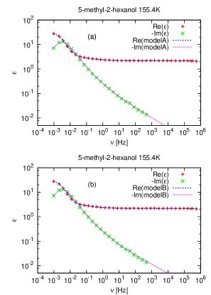
Figure 1: (Color online) Simultaneous fits of real and imaginary part with model A (upper figure) and model B (lower figure) for 5-methyl-2-hexanol at $155.4\,{\rm K}$. Both models show an excellent fitting capability. The data are from Kalinovskaya .

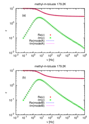
Figure 2: (Color online) Simultaneous fits of real and imaginary part with model A (upper figure) and model B (lower figure) for methyl-m-toluate at $179.2\,{\rm K}$. Model A can fit the data over the whole spectral range of 7 decades, which is more then with Havriliak-Negami which uses the same number of fit parameters. With this data we obtain the broadest fit with model A. The data are from RoskildeChemPhys2009 .

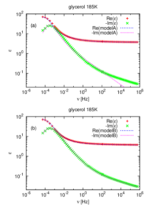
Figure 3: (Color online) Simultaneous fits of real and imaginary part with model A (upper figure) and model B (lower figure) for glycerol at $185\,{\rm K}$. While model A is not able to fit the data well, model B still gives an excellent fit over 10 decades. The data are from LoidlGlycerol .

V Temperature dependence of the parameters

Because the data have been fitted at different temperatures we are able to observe the temperature dependence of the fitting parameters. For $\tau_{1}$ and $\tau_{2}$ we perform Vogel-Tammann-Fulcher fits provided by equation (13). Note that in our notation $\varepsilon=\varepsilon^{\prime}-i\varepsilon^{\prime\prime}$. From the fits we obtain the Vogel-Fulcher temperatures $T_{\rm VF1}$ and $T_{\rm VF2}$ as well as the fragility parameters $D_{1}$ and $D_{2}$ for the relaxation times $\tau_{1}$ and $\tau_{2}$ for model A and model B (see Table 2).

Table 2: List of the fit parameters $T_{\rm VF}$, $D$ and $\tau_{0}$ for various materials.

material model $T_{\rm VF1}$ $T_{\rm VF2}$ $D_{1}$ $D_{2}$ $\tau_{01}$ $\tau_{02}$ 5-methyl-2-hexanol A $89.2\,{\rm K}$ $92.1\,{\rm K}$ $25.5$ $22.1$ $3.53\times 10^{-13}\,{\rm s}$ $7\times 10^{-14}\,{\rm s}$ 5-methyl-2-hexanol B $88.3\,{\rm K}$ $101.6\,{\rm K}$ $26.3$ $15.3$ $5.21\times 10^{-13}\,{\rm s}$ $5.77\times 10^{-12}\,{\rm s}$ glycerol A $127.8\,{\rm K}$ $131.5\,{\rm K}$ $17.1$ $14.9$ $3.7\times 10^{-14}\,{\rm s}$ $3.23\times 10^{-14}\,{\rm s}$ glycerol B $152.7\,{\rm K}$ $137.8\,{\rm K}$ $6.68$ $11.9$ $2.9\times 10^{-10}\,{\rm s}$ $2.15\times 10^{-13}\,{\rm s}$ methyl-m-toluate A $71.2\,{\rm K}$ $71.2\,{\rm K}$ $93.2$ $93.2$ $4.35\times 10^{-28}\,{\rm s}$ $1.54\times 10^{-28}\,{\rm s}$ methyl-m-toluate B $67.2\,{\rm K}$ $85.6\,{\rm K}$ $102.2$ $53.6$ $9.0\times 10^{-28}\,{\rm s}$ $1.13\times 10^{-22}\,{\rm s}$

For all fits we see a temperature dependence of the relaxation times $\tau_{1}$ and $\tau_{2}$ (Fig. 4 - Fig. 6) that follows the Vogel-Tammann-Fulcher fitting function remarkably well. The relaxation times also show a clear downward trend as the temperature increases, which confirms that $\tau$, $\tau_{1}$ and $\tau_{2}$ are physically meaningful and can be interpreted as relaxation times even tough they appear with a non-integer power in equations (11) and (12).

The parameters $\alpha$, $\alpha_{1}$ and $\alpha_{2}$ also show a temperature dependence. In the case of 5-methyl-2-hexanol (Fig. 4) there is an increase of $\alpha$ with temperature until a plateau near $\alpha=1$ is reached. This effect comes from the decreasing slope of the excess wing with increasing temperature. In the fitting function of model A this behavior can be achieved by increasing $\alpha$. For the same material there is an apparent increase of $\alpha_{2}$ between $154\,{\rm K}$ ($6.49\,{\rm K}^{-1}$) and $287\,{\rm K}$ ($3.48\,{\rm K}^{-1}$) which has the same origin as the increase in $\alpha$ in model A. By increasing $\alpha_{2}$ the excess wing becomes less steep. The plateau at $190\,{\rm K}$ ($5.26\,{\rm K}^{-1}$) and above comes from the fact that the fits at those temperatures are done mainly for the $\alpha$-peak since the excess wing is not visible.

For glycerol and methyl-m-toluate there is also a clear temperature dependence of $\alpha$, $\alpha_{1}$ and $\alpha_{2}$ (Fig. 5 and Fig. 6). The trend is however reversed in comparison to 5-methyl-2-hexanol. This comes from the increasing slope of the excess wing with increasing temperature. This behavior can be achieved in the fit functions by decreasing $\alpha$, respectively $\alpha_{2}$.

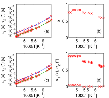
Figure 4: (Color online) Temperature dependence of the fitting parameters for 5-methyl-2-hexanol for model A (upper panels) and model B (bottom panels) together with Vogel-Tammann-Fulcher fits.

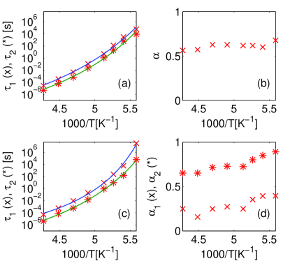
Figure 5: (Color online) Temperature dependence of the fitting parameters for glycerol for model A (upper panels) and model B (bottom panels) together with Vogel-Tammann-Fulcher fits.

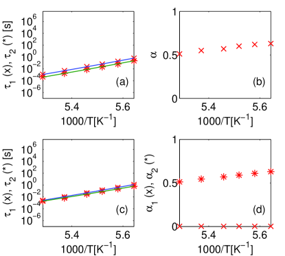
Figure 6: (Color online) Temperature dependence of the fitting parameters for methyl-m-toluate for model A (upper panels) and model B (bottom panels) together with Vogel-Tammann-Fulcher fits.

VI Representation of the solutions as functions of time

In CandelaresiMaster08 we obtained the analytical solution of a fractional differential equation of rational order, which we use to analyze our fitting results for model A and model B. For a general solution of equations (11) and (12) with arbitrary real $\alpha_{i}$ see hil09d . The restriction to rational $\alpha_{i}$ is not a drawback, since we can approximate $\alpha_{1}$ and $\alpha_{2}$ by a rational value on a grid between 0 and 1. This number of grid points is chosen to be 20, which keeps computation times reasonably limited as the computing time increases quadratically with the lowest common denominator of $\alpha$ with 1.

The solution for $f(t)$ for model B is a sum of Mittag-Leffler type functions:

$$f(t)=\sum_{j=1}^{N}B_{j}\sum_{k=0}^{N-1}c_{j}^{N-k-1}\mbox{$E\left(-k/N,c_{j}^{N};t\right)$},$$ (14)

where $N$ is the smallest number for which both $\alpha_{1}N$ and $\alpha_{2}N$ are integers. The coefficients $c_{j}$ are the zeros of the characteristic polynomial

$$c^{N}+\tau_{1}^{\alpha_{1}}c^{\alpha_{1}N}+\tau_{2}^{\alpha_{2}}c^{\alpha_{2}N}+1=0,$$ (15)

the function $E\left(\nu,a;t\right)$ is defined as MillerRoss

$$\mbox{$E\left(\nu,a;t\right)$}=t^{\nu}\sum_{k=0}^{\infty}\frac{(at)^{k}}{\Gamma(\nu+k+1)}.$$ (16)

The coefficients $B_{j}$ are the solutions of the linear system of equations

$$\sum\limits_{k=1}^{N}c_{k}^{i}B_{k}=0,$$ (17)

$$0\leq i\leq N-\alpha_{1}N-1$$

$$\sum\limits_{k=1}^{N}(c_{k}^{i}+\tau_{1}^{\alpha_{1}}c_{k}^{i-N+\alpha_{1}N})B_{k}=0,$$ (18)

$$N-\alpha_{1}N\leq i\leq N-\alpha_{2}N-1$$

$$\sum\limits_{k=1}^{N}(c_{k}^{i}+\tau_{1}^{\alpha_{1}}c_{k}^{i-N+\alpha_{1}N}+\tau_{2}^{\alpha_{2}}c_{k}^{i-N+\alpha_{2}N})B_{k}=0,$$ (19)

$$N-\alpha_{2}N\leq i\leq N-2.$$

This solution is only valid if all the roots $c_{j}$ of the characteristic polynomial in (15) are distinct, which is checked in the computations. Since the linear system of equations (17)-(19) is underdetermined we choose one fundamental solution for $\{B_{j}\}$ and a multiplication factor for $f(t)$ such that $f(0)=1$.

The analytical solutions are plotted for glycerol at $195\,{\rm K}$ (Fig. 7). The fitting values for $\tau$ for model A are $\tau_{1}=4.991\,{\rm s}$ and $\tau_{2}=1.089\,{\rm s}$. Both values lie in the time interval where the relaxation occurs, which confirms the interpretation of these fitting parameters as relaxation times. For model B the fitted times are $\tau_{1}=9.729\,{\rm s}$ and $\tau_{2}=0.92\,{\rm s}$. So $\tau_{2}$ marks the onset of the relaxation and $\tau_{1}$ the end.

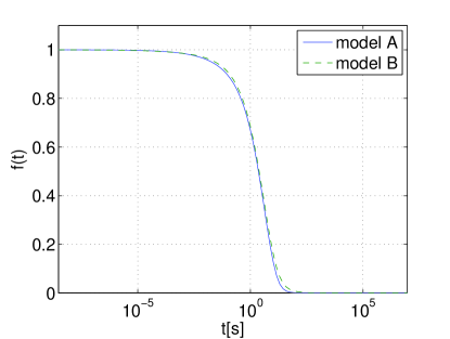
Figure 7: (Color online) The solutions of the fractional initial value problems (6) and (7) with $f(0)=1$ using the fit parameters for model A and model B for glycerol at $195\,{\rm K}$.

We note that the fractional derivatives appearing in the initial value problem (7) can be generalized to fractional derivatives of arbitrary type $\beta$ introduced in hil00a and defined as

$$\mbox{${\rm D}$}{}^{\nu,\beta}f(t)=\mbox{${\rm I}$}{}^{(1-\beta)(\lceil\nu\rceil-\nu)}\mbox{${\rm D}$}{}^{\lceil\nu\rceil}\mbox{${\rm I}$}{}^{\beta(\lceil\nu\rceil-\nu)}f(t),$$ (20)

$$0\leq\beta\leq 1.$$

For the case $\beta=1$ it reduces to the Riemann-Liouville fractional derivative, while for $\beta=0$ to the Caputo-type derivative Caputo67 . Because

$$\mbox{${\rm D}$}{}^{\nu,\beta}\mbox{$E\left(\mu,a;t\right)$}=\mbox{${\rm D}$}{}^{\nu,\gamma}\mbox{$E\left(\mu,a;t\right)$},$$ (21)

$$0\leq\beta,\gamma\leq 1,\quad\mu>-1,\quad\nu\geq 0,$$

the solution of our initial value problem does not change by replacing the Riemann-Liouville fractional derivatives with these generalized Riemann-Liouville fractional derivatives of type $\beta$.

VII Conclusions

The two fractional relaxation models (model A and model B) are shown to fit well dielectric spectroscopy data for various glass forming materials over a range of at least 5 orders of magnitude for model A and 10 orders of magnitude for model B. For 5-methyl-2-hexanol and methyl-m-toluate model A can fit data over a range of 6 and 7 orders of magnitude. This is a significant improvement over conventional fitting formulae like Havriliak-Negami and Cole-Cole which need to be superimposed in order to fit data at the same range. Conventional fitting formulae require 6 parameters in contrast to 3 for our model A and 4 for our model B. Another advantage of the fractional relaxation models is that the fitting formulas follow from an underlying general theory based on composition of fractional semigroups and their infinitesimal generators, which is not the case for Havriliak-Negami or Cole-Cole functions.

VIII Acknowledgements

We thank Sebastian Schmiescheck for converting data into a workable format.

References

- (1) P. Lunkenheimer, U. Schneider, R. Brand, and A. Loid, “Glassy dynamics,” Contemporary Physics, vol. 41, pp. 15–36, 2000.
- (2) P. Lunkenheimer, A. Pimenov, B. Schiener, R. Böhmer, and A. Loidl, “High-frequency dielectric spectroscopy on glycerol,” EPL (Europhysics Letters), vol. 33, no. 8, p. 611, 1996.
- (3) S. Corezzi, S. Capaccioli, G. Gallone, M. Lucchesi, and P. A. Rolla, “Dynamics of a glass-forming triepoxide studied by dielectric spectroscopy,” Journal of Physics: Condensed Matter, vol. 11, no. 50, pp. 10297–10314, 1999.
- (4) R. Behrends, K. Fuchs, U. Kaatze, Y. Hayashi, and Y. Feldman, “Dielectric properties of glycerol/water mixtures at temperatures between 10 and 50 [degree]c,” The Journal of Chemical Physics, vol. 124, no. 14, p. 144512, 2006.
- (5) S. Corezzi, M. Beiner, H. Huth, K. Schröter, S. Capaccioli, R. Casalini, D. Fioretto, and E. Donth, “Two crossover regions in the dynamics of glass forming epoxy resins,” The Journal of Chemical Physics, vol. 117, no. 5, pp. 2435–2448, 2002.
- (6) O. E. Kalinovskaya and J. K. Vij, “The exponential dielectric relaxation dynamics in a secondary alcohol’s supercooled liquid and glassy states,” The Journal of Chemical Physics, vol. 112, no. 7, pp. 3262–3266, 2000.
- (7) U. Schneider, P. Lunkenheimer, R. Brand, and A. Loidl, “Broadband dielectric spectroscopy on glass-forming propylene carbonate,” Phys. Rev. E, vol. 59, no. 6, pp. 6924–6936, 1999.
- (8) P. Lunkenheimer, A. Pimenov, M. Dressel, Y. G. Goncharov, R. Böhmer, and A. Loidl, “Fast dynamics of glass-forming glycerol studied by dielectric spectroscopy,” Phys. Rev. Lett., vol. 77, no. 2, pp. 318–321, 1996.
- (9) A. Puzenko, Y. Hayashi, Y. Ryabov, I. Balin, Y. Feldman, U. Kaatze, and R. Behrends, “Relaxation dynamics in glycerol-water mixtures: I. glycerol-rich mixtures,” Journal of Physical Chemistry B, vol. 109, no. 12, pp. 6031–6035, 2005.
- (10) Y. Hayashi, A. Puzenko, I. Balin, Y. Ryabov, and Y. Feldman, “Relaxation dynamics in glycerol-water mixtures. 2. mesoscopic feature in water rich mixtures,” Journal of Physical Chemistry B, vol. 109, no. 18, pp. 9174–9177, 2005.
- (11) T. Hecksher, A. I. Nielsen, N. B. Olsen, and J. C. Dyre, “Little evidence for dynamic divergences in ultraviscous molecular liquids,” Nat. Phys., vol. 4, pp. 737 – 741, 2008.
- (12) A. I. Nielsen, T. Christensen, B. Jakobsen, K. Niss, N. B. Olsen, R. Richert, and J. C. Dyre, “Prevalence of approximate sqrt(t) relaxation for the dielectric alpha process in viscous organic liquids,” The Journal of Chemical Physics, vol. 130, no. 15, p. 154508, 2009.
- (13) F. Kremer and A. Schönhals, Broadband Dielectric Spectroscopy. Berlin: Springer Verlag, 2003.
- (14) W. Götze, “The essentials of the mode-coupling theory for glassy dynamics,” Condensed Matter Physics, vol. 1, no. 4, p. 873, 1998.
- (15) D. R. Reichman and P. Charbonneau, “Mode-coupling theory,” Journal of Statistical Mechanics: Theory and Experiment, vol. 2005, no. 05, p. P05013, 2005.
- (16) S. Havriliak and S. Negami, “A complex plane analysis of -dispersions in some polymer systems,” Journal of Polymer Science Part C: Polymer Symposia, vol. 14, no. 1, pp. 99–117, 1966.
- (17) R. Hilfer, “Experimental evidence for fractional time evolution in glass forming materials,” Chemical Physics, vol. 284, no. 1–2, pp. 399 – 408, 2002.
- (18) R. Hilfer, “On fractional relaxation,” Fractals, vol. 11, pp. 251–257, 2003.
- (19) H. Fröhlich, Theory of Dielectrics: Dielectric Constant and Dielectric Loss. Oxford University Press, 1949.
- (20) K. S. Cole and R. H. Cole, “Dispersion and absorption in dielectrics i. alternating current characteristics,” The Journal of Chemical Physics, vol. 9, no. 4, pp. 341–351, 1941.
- (21) D. W. Davidson and R. H. Cole, “Dielectric relaxation in glycerol, propylene glycol, and n-propanol,” The Journal of Chemical Physics, vol. 19, no. 12, pp. 1484–1490, 1951.
- (22) R. Hilfer, “Classification theory for anequilibrium phase transitions,” Phys. Rev. E, vol. 48, pp. 2466–2475, 1993.
- (23) R. Hilfer, “Fractional dynamics, irreversibility and ergodicity breaking,” Chaos Solitons & Fractals, vol. 5, pp. 1475–1484, 1995.
- (24) R. Hilfer, “Foundations of fractional dynamics,” Fractals, vol. 3, pp. 549–556, 1995.
- (25) R. Hilfer, “An extension of the dynamical foundation for the statistical equilibrium concept,” Physica A, vol. 221, pp. 89–96, 1995.
- (26) R. Hilfer, Applications of Fractional Calculus in Physics. Singapore: World Scientific Publ. Co., 2000.
- (27) R. Hilfer, “Fractional time evolution,” in Applications of Fractional Calculus in Physics (R. Hilfer, ed.), p. 87, Singapore: World Scientific Publ. Co., 2000.
- (28) R. Hilfer, “Fitting the excess wing in the dielectric -relaxation of propylene carbonate,” Journal of Physics: Condensed Matter, vol. 14, pp. 2297–2301, 2002.
- (29) R. Hilfer, “Remarks on fractional time,” in Time, Quantum and Information (L. Castell and O. Ischebeck, eds.), p. 235, Berlin: Springer Verlag, 2003.
- (30) R. Hilfer, “On fractional diffusion and continuous time random walks,” Physica A, vol. 329, pp. 35–40, 2003.
- (31) R. Hilfer, “Threefold introduction to fractional derivatives,” in Anomalous Transport: Foundations and Applications (R. Klages, G. Radons, and I. Sokolov, eds.), pp. 17–73, Wiley-VCH, 2008.
- (32) R. Hilfer, “Foundations of fractional dynamics: A short account,” in Fractional Dynamics: Recent Advances (J. Klafter, S. Lim, and R. Metzler, eds.), p. 207, Singapore: World Scientific Publ. Co., 2001.
- (33) R. Hilfer, Y. Luchko, and Z. Tomovski, “Operational method for the solution of fractional differential equations with generalized Riemann-Liouville fractional derivatives,” Fractional Calculus and Applied Analysis, vol. 12, p. 299, 2009.
- (34) K. S. Miller and B. Ross, An Introduction to fractional Calculus and fractional Differential Equations. Wiley-Interscience, 1993.
- (35) S. Candelaresi, “Fraktionale ansätze in dielektrischer breitbandspektroskopie,” Master’s thesis, 2008.
- (36) M. Caputo, “Linear models of dissipation whose q is almost frequency independent-ii,” Geophysical Journal of the Royal Astronomical Society, vol. 13, no. 5, pp. 529–539, 1967.