Thermalization in one- plus two-body ensembles for dense interacting boson systems

Abstract

Employing one plus two-body random matrix ensembles for bosons, temperature and entropy are calculated, using different definitions, as a function of the two-body interaction strength $\lambda$ for a system with 10 bosons $(m=10)$ in five single particle levels $(N=5)$. It is found that in a region $\lambda\sim\lambda_{t}$, different definitions give essentially same values for temperature and entropy, thus defining a thermalization region. Also, $(m,N)$ dependence of $\lambda_{t}$ has been derived. It is seen that $\lambda_{t}$ is much larger than the $\lambda$ values where level fluctuations change from Poisson to GOE and strength functions change from Breit-Wigner to Gaussian.

I Introduction

In recent years, the study of thermalization in isolated finite many-body quantum systems, due to inter-particle interactions, has received considerable interest Rigol-08 ; Rigol-09 ; Rigol-11 ; San-10 ; San-12a ; San-12b ; Kota-11 . This interest has arisen mainly due to major developments in experimental study of many-particle quantum systems such as ultracold gases trapped in optical lattices Expt . In particular, Rigol and Santos group employed interacting spin-$1/2$ systems (fermions and hard core bosons) on a lattice and examined various issues such as the role of localization and chaos, statistical relaxation, eigenstate thermalization, ergodicity principle and so on Rigol-08 ; Rigol-09 ; Rigol-11 ; San-10 ; San-12a ; San-12b . Horoi et al. Ho-95 and Kota and Sahu Kota-02 examined occupancies and different definitions of entropy for ²⁸Si and ²⁴Mg respectively, using nuclear shell model with realistic interactions. It was shown that the nuclei would be in the thermodynamic regime in general, when these are away from the ground state. Similarly, Casati’s group examined in the past, Fermi-Dirac (FD) representability of occupation numbers for a spin-$1/2$ system on a two-dimensional lattice Cas-01 and more recently studied thermalization in spin-$1/2$ systems, locally coupled to an external bath, using an approach based on the time-dependent density-matrix renormalization group method Cas-10 . Let us add that, as emphasized by Santos et al. San-12b , it is possible to realize interacting spin-$1/2$ models experimentally in optical lattices.

On the other hand, thermalization in fermionic systems has been studied in some detail using embedded Gaussian orthogonal ensemble of one- plus random two-body matrix ensembles [called EGOE(1+2)] Ko-01 ; Go-11 , i.e. random matrix ensembles in many-fermion spaces generated by random two-body interactions in presence of a mean-field. The EGOEs form generic models for finite isolated interacting many-fermion systems (for boson systems these are called BEGOE with ‘B’ for bosons) and they model what one may call quantum many-body chaos Ko-01 ; Go-11 . The role of interactions in thermalization can be investigated by varying the interaction strength in these models. For example, for spin-less fermion systems, Flambaum et al. showed that EGOE(1+2) exhibits a region of thermalization Flam-97 and found the criterion for the occupancies to follow FD distributionFlam-97 ; Flam-96 . Later, using EGOE both for spin-less fermions and fermions with spin Kota-02 ; An-04 ; Ma-10 , thermalization region generated by random interactions has been established by analyzing different definitions for entropy. Going beyond these, in a more detail study, thermalization has been investigated within EGOE(1+2) for spin-less fermions by Kota et al. Kota-11 using the ergodicity principle for the expectation values of different types of operators. Recently, Santos et al. compared results of spin-less EGOE(1+2) for statistical relaxation Fl-01 with those from spin-$1/2$ lattice models San-12a ; San-12b .

Turning to interacting boson systems, thermalization was investigated by Borgonovi et al. Borg-98 using a simple symmetrized coupled two-rotor model. They explored different definitions of temperature and compared the occupancy number distribution with the Bose-Einstein (BE) distribution. They conclude that: “For chaotic eigenstates, the distribution of occupation numbers can be approximately described by the BE distribution, although the system is isolated and consists of two particles only. In this case a strong enough interaction plays the role of a heat bath, thus leading to thermalization”. As BEGOEs PDPK ; Ch-03 ; Ch-04 ; Ma-arxiv ; Ag-01 are generic models for finite isolated interacting many-boson systems, it is important to investigate thermalization using these ensembles.

Embedded Gaussian orthogonal ensemble of one- plus random two-body matrix ensembles for spin-less boson systems is called BEGOE(1+2) and this ensemble was introduced and analyzed for spectral and wave-function properties in PDPK ; Ch-03 ; Ch-04 . For $m$ bosons in $N$ single particle (sp) levels, in addition to dilute limit (defined by $m\rightarrow\infty,N\rightarrow\infty$ and $m/N\rightarrow 0$), another limiting situation, namely the dense limit (defined by $m\to\infty$, $N\to\infty$ and $m/N\to\infty$) is also feasible. This limiting situation is absent for fermion systems. Therefore the focus was on the dense limit in BEGOE investigations PDPK ; Ch-03 ; Ch-04 ; Ma-arxiv ; Ag-01 . In the strong interaction limit, two-body part of the interaction dominates over one-body part and hence BEGOE(1+2) reduces to BEGOE(2). Some of the generic results established for BEGOE(1+2) are as follows: (i) eigenvalue density approaches Gaussian form PDPK ; KP-80 ; (ii) for strong enough interaction, there is average-fluctuation separation in eigenvalues PDPK ; Leclair ; (iii) similarly, the ensemble is ergodic in the dense limit with sufficiently large $N$ Ch-03 and there will be deviations for small $N$ Ag-01 ; (iv) as the strength of the two-body interaction, $\lambda$, increases, there is Poisson to GOE transition in level fluctuations at $\lambda=\lambda_{c}$ Ch-03 and with further increase in $\lambda$, there is Breit-Wigner to Gaussian transition in strength functions at $\lambda=\lambda_{F}$ Ch-04 . The main result of the present Letter is the demonstration that finite dense interacting boson systems generate a third chaos marker $\lambda_{t}$ [as in fermionic EGOE(1+2) ensembles], a point or a region where different definitions of entropy, temperature, specific heat and other thermodynamic variables give the same results, i.e. where thermalization occurs.

In this Letter, we present results for thermalization in dense interacting bosonic systems by varying the strength parameter $\lambda$ of the two-body interaction in the BEGOE(1+2) Hamiltonian given by $H=h(1)+\lambda V(2)$. Here $h(1)$ is one-body part of the interaction, defined by single particle energies (SPEs) $\varepsilon_{k}$ ($k$ = 1 to $N$) for $N$ sp levels while the two-body interaction $V(2)$ is defined by the two-body matrix elements (TBMEs) denoted as $V_{ijkl}=\left\langle(ij)|V(2)|(kl)\right\rangle$. In the present study SPEs are taken as independent gaussian random variables with mean equal to $k$ and variance equal to $1/2$. Similarly, TBMEs are taken as independent gaussian random variables with zero mean and variance=1 for off diagonal TBMEs and variance=2 for diagonal TBMEs. Construction of the $m$-boson Hamiltonian, $H(m)$, and thereby the BEGOE(1+2) ensemble in $m$-particle space with matrix dimension $d={N+m-1\choose m}$ was described completely in PDPK ; Ch-04 . The results, presented here, have been obtained by fully diagonalizing 100-members of a BEGOE(1+2) ensemble with 10 bosons in 5 sp levels for each value of $\lambda$. The dimensionality of the system is $d=1001$. (we have also carried out calculations for 10 bosons in 4 sp levels and similar results were obtained, but they are not presented here as this is a much smaller example, $d=286$). The ensemble average is carried out by making the spectra of each member of the ensemble zero centered ($\epsilon$ is centroid) and scaled to unit width ($\sigma$ is width).

The paper is organized as follows. In Section II, different definitions of temperature are given and results obtained by varying the two-body interaction strength in BEGOE(1+2) are described. Similarly, results obtained using three different definitions for entropy, are described in Section III. They allow us to define the thermalization marker $\lambda_{t}$. In Section IV, duality point is discussed, using information entropy and strength functions, in the two extreme basis defined by $h(1)$ and $V(2)$ operators and the $(m,N)$ dependence of the marker $\lambda_{t}$ is derived. Finally, Section V gives conclusions.

II Temperature: Definitions and Results

Temperature can be defined in a number of different ways in the standard thermodynamical treatment. These definitions of temperature are known to give same result in the thermodynamical limit i.e. near a region where thermalization occurs Rigol-08 . In this section, four different definitions of temperature ($T=\beta^{-1}$), described below, have been used to compute the temperature of finite dense interacting boson systems as a function of energy as well as a function of the two-body interaction strength.

• $\beta_{c}$: defined using the canonical expression, between energy and temperature which allows standard thermodynamical description for the quantum system, is given by

  $${\left\langle E\right\rangle}_{\beta_{c}}=\frac{\sum_{i}E_{i}\;\exp[-\beta_{c}\;E_{i}]}{\sum_{i}\exp[-\beta_{c}\;E_{i}]}\;;$$ (1)

  where $E_{i}$ are the eigen-energies of the Hamiltonian. With above relation, ${\left\langle E\right\rangle}$ can be obtained at given $\beta_{c}$ using all the eigen-energies of the system.

• $\beta_{fit}$: defined using occupation numbers obtained by making use of the standard canonical distribution is given by,

  $${\left\langle n(E)_{k}\right\rangle}=\frac{\sum_{i}n(E_{i})_{k}\;\exp[-\beta_{fit}\;E_{i}]}{\sum_{i}\exp[-\beta_{fit}\;E_{i}]}.$$ (2)

  Here $k$ is sp level index and $i$ is eigen-energy index. Using expectation values of occupancies calculated for all eigen-states and exact eigen-energies, $\beta_{fit}$ can be computed by considering Eq. (2) as one parameter fitting expression and with the constraint, $\sum_{k}n(E)_{k}=m$.

• $\beta_{BE}$: defined using BE distribution for the occupation numbers is given by,

  $$n(E)_{k}^{BE}=1/\{\exp[\beta_{BE}(E)\;(\varepsilon_{k}-\mu(E))]-1\}.$$ (3)

  Here $\mu$ is a chemical potential. Although, this expression is derived for many-body non-interacting particles in contact with a thermostat, it is shown that conventional quantum statistics can appear even in isolated systems with relatively few particles, provided a proper renormalization of energy is taken Flam-97 ; Flam-96 . Comparing numerical data of expectation values of occupancies at a particular eigenenergy and given SPEs, the unknowns $\beta_{BE}$ and $\mu$ in the BE distribution with constraint $\sum_{k}n(E)_{k}^{BE}=m$ can be obtained.

• $\beta_{T}$: defined using state density, $\rho(E)$, of the total Hamiltonian. The thermodynamic entropy is defined as $S^{ther}(E)=\log[\rho(E)]$. The $\beta_{T}$ can be computed using $\beta_{T}=\frac{d\ln[\rho(E)]}{dE}$. Here not that, for BEGOE(1+2), the form of state density is very close to Gaussian irrespective of the value of two-body interaction strength PDPK ; KP-80 .

Figure 1 shows ensemble averaged values of $\beta$, computed via definitions described above, for a 100 member BEGOE(1+2) ensemble with $m=10$ and $N=5$ as a function of normalized energy, $\hat{E}=(E-\epsilon)/\sigma$, for various $\lambda$ values. Here, we compare numerical values of $\beta$ from $\hat{E}=-1.5$ to the center of the spectrum, where temperature is infinity. The edges of the spectrum have been avoided for the following reasons: (i) density of states is small near the edges of the spectrum; (ii) eigenstates near edges are not fully chaotic. The $\beta$ values are obtained for all members separately and then ensemble average is carried out taking bin-size equal to 0.1. Since the state density for BEGOE(1+2) is Gaussian irrespective of $\lambda$ values, $\beta_{T}$ as a function of energy gives straight line. In Fig. 1, $\beta_{T}$ results are shown in the plots by dotted lines. It is clearly seen from Fig. 1 that for the interaction strength $\lambda<\lambda_{c}$ (For $(m,N)=(10,5)$, $\lambda_{c}\sim 0.02$ and $\lambda_{F}\sim 0.05$, see ref.Ch-03 ), there is significant difference between the numerical values of $\beta$ obtained via various definitions of temperature. Going further beyond $\lambda_{c}$ ($\lambda_{c}<\lambda<\lambda_{F}$) where GOE fluctuations in state density sets in but the eigenstates are still not fully chaotic, the $\beta$ values obtained via canonical expressions, defined by Eq.(1) and (2), give good agreement near the center of the spectrum. There are deviations near low temperature region. Near the region $\lambda=\lambda_{F}$ and beyond, the eigenstates become fully chaotic giving very good agreement between the numerical values of $\beta_{c}$ and $\beta_{fit}$. The inverse temperature $\beta_{BE}$ is obtained by solving microcanonical definition given by Eq. (3), with SPEs taken as independent Gaussian random variables and results are shown in the plots by red stars. In the region $\lambda<\lambda_{F}$, inverse temperature $\beta_{BE}$, found from BE distribution turns out to be completely different from $\beta$ values obtained using other definitions. As in this region, the structure of eigenstates is not chaotic enough, leading to strong variation in the distribution of the occupation numbers and thus strong fluctuations in $\beta_{BE}$. Moreover, near the center of the spectrum (i.e. as $T\to\infty$), the value of denominator in Eq. (3) becomes very small, which leads to large variation in $\beta_{BE}$ values from member to member. Further increase in $\lambda>\lambda_{F}$, in the classically chaotic region, the occupation number distribution becomes statistically stable with respect to the choice of eigenstate and at one point $\lambda=\lambda_{t}$, temperatures defined using canonical and microcanonical definitions give same result, i.e. $\beta_{fit}\simeq\beta_{BE}$. This lead to same values of temperature giving the thermodynamic marker $\lambda_{t}$. In the strong interaction domain ($\lambda\geq\lambda_{t}$), the match between $\beta_{BE}$ with other $\beta$ values is not good. This is due to neglect of induced SPEs, $\widetilde{\varepsilon_{k}}=\frac{m-1}{N+2}\sum_{j}V_{kjkj}$, from two-body interaction KP-80 . When the interaction is weak, induced SPEs part is small but in strong interaction domain their contribution is important. Adding induced SPEs part into SPEs, $\beta_{BE}$ is obtained by taking a proper renormalization of energy and results are also presented in Fig. 1 for $\lambda$ values 0.13 and 0.2 by green filled circles. Here, $\beta_{BE}$ values come quite close to other $\beta$ values. We found that the match between different values of $\beta$ is good near $\lambda=\lambda_{t}=0.13$. In the next section, we present our results for similar study using the different definitions of entropy.

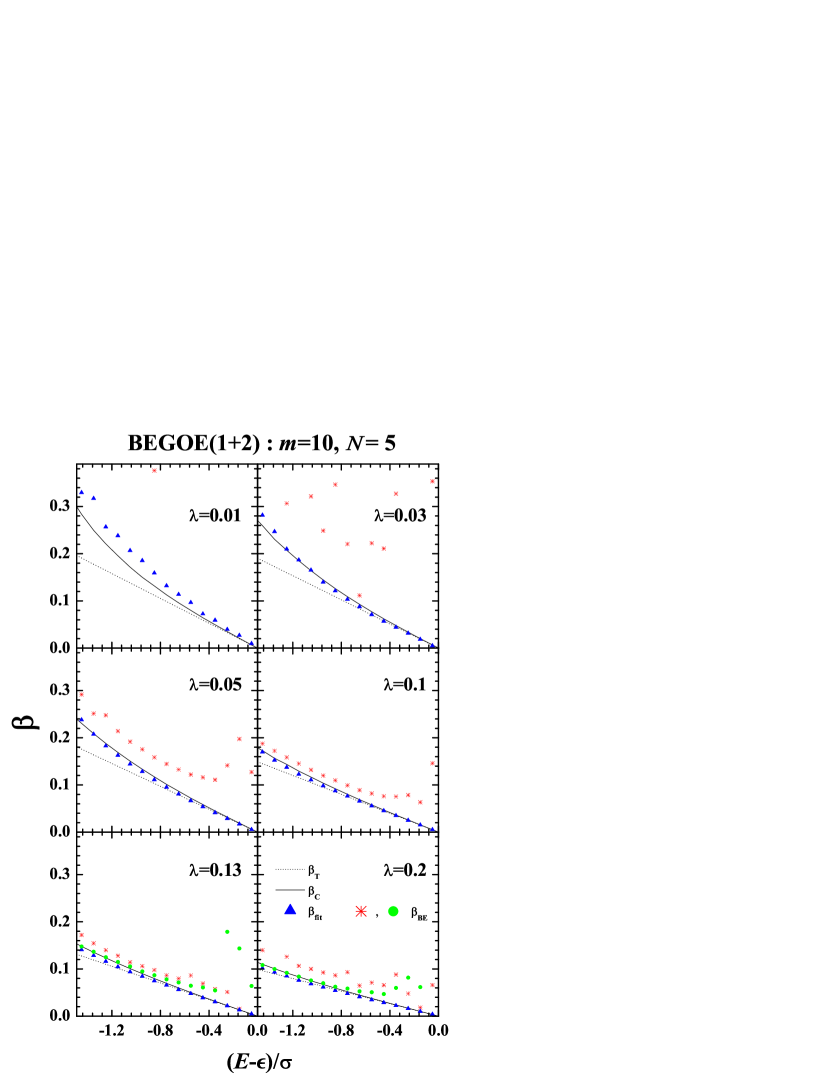
Figure 1: (Color online) Ensemble averaged values of inverse temperature ($\beta$) as a function of normalized energy, $(E-\epsilon)/\sigma$, for different values of two body interaction strength $\lambda$, calculated using a 100 member BEGOE(1+2) ensemble with $m=10$ and $N=5$. Here in calculations, different definitions of inverse of temperature are used. In the calculations, SPEs, drawn from independent real Gaussian random variables, are employed. Results are also shown, in the plots for $\lambda=0.13$ and $0.2$, for $\beta_{BE}$ by green filled circles, in which induced SPEs from the two-body interaction are taken into account.

III Entropy: Definitions and Results

In this section, to identify the thermalization region and hence value of the third marker $\lambda_{t}$ for BEGOE(1+2), we consider following three definitions of entropy.

• Thermodynamic entropy, obtained using the state density $\rho(E)$, as a function of of energy eigenvalues; $S^{ther}(E)=\log[\rho(E)]$.

• Information entropy in the mean-field basis defined by $S^{info}(E)=-\sum_{i}^{d}{|C_{i}^{E}|^{2}\log(|C_{i}^{E}|^{2})}$, here $|C_{i}^{E}|^{2}$ is the probability of basis state $i$ in the eigenstate at energy $E$.

• Single particle entropy, obtained by calculating the occupancy of different single-particle states, as a function of energy eigenvalues; $S^{sp}(E)=-\sum_{k}{\left\langle n_{k}(E)\right\rangle}\log({\left\langle n_{k}(E)\right\rangle})$. Here the summation is over all $N$ sp levels and $n_{k}(E)$ is the occupancy of the $k$-th sp level at energy $E$.

We use following measure, defined using above definitions of entropy Kota-11 , to obtain $\lambda_{t}$:

$$\Delta_{s}(\lambda)=\frac{\sqrt{\int^{\infty}_{-\infty}[(R^{info}_{E}-R^{ther}_{E})^{2}+(R^{sp}_{E}-R^{ther}_{E})^{2}]dE}}{\int^{\infty}_{-\infty}R^{ther}_{E}dE},$$ (4)

where $R^{\alpha}_{E}=\exp[S^{\alpha}(E)-S^{\alpha}_{max}]$. In the thermodynamic region the values of the different entropies will be very close to each other, hence the minimum of $\Delta_{s}$ gives the value of $\lambda_{t}$. In Fig. 2, results shown for ensemble averages $\overline{\Delta_{s}(\lambda)}$ (blue stars) obtained for a $100$ member BEGOE(1+2) ensemble with $10$ bosons in $5$ sp levels as a function of $\lambda$. The second vertical dash-line indicates the position of $\lambda_{t}$ where ensemble average $\overline{\Delta_{s}(\lambda)}$ is minimum. For the present example, we obtained $\lambda_{t}\simeq 0.13$. This value of $\lambda_{t}$ is same as obtained in Section II, at which different definitions of temperature give same values.

In the past it is demonstrated that for BEGOE(1+2), as the strength $\lambda$ of the two-body interaction increases, there is Poisson to GOE transition in level fluctuations at $\lambda=\lambda_{c}$ Ch-03 . In order to show that $\lambda_{c}<<\lambda_{t}$, we study the nearest neighbor spacing distribution (NNSD) as a function of $\lambda$ to detect the position of marker $\lambda_{c}$. It is well known that when the system is in integrable domain, the form of NNSD is close to the Poisson distribution, i.e, $P(s)=\exp(-s)$, while in chaotic domain, the form of NNSD is the Wigner surmise, $P(s)=(\pi s/2)\;\exp(-\pi s^{2}/4)$. To interpolate between these two extremes, we use Brody distribution Brody-81 , $P(s,\omega)=A_{\omega}(\omega+1)s^{\omega}\exp(-A_{\omega}\;s^{\omega+1})$. Here $\omega$ is called the Brody parameter and $A_{\omega}$ is a normalization constant. If the spectral fluctuations are close to the Poisson type, $\omega=0$, or to the Wigner surmise with $\omega=1$. The position of the chaos marker $\lambda_{c}$ is fixed by the condition $\omega(\lambda)=1/2$. Here, the NNSD is obtained, using the unfolding procedure described in PDPK , with the smooth density taken as a corrected Gaussian with corrections involving up to $6$th order moments of the density function. In Fig. 2, Ensemble averaged values of $\overline{\omega(\lambda)}$ are shown by filled triangles for a $100$ member BEGOE(1+2) ensemble with ($m,N$)=($10$,$5$) as a function of two-body interaction strength $\lambda$. The $\lambda_{c}$ is shown by vertical dash line in the Fig. 2. Here, different criterion is used, than in Ch-03 , to obtain $\lambda_{c}$ although match is very good. The results clearly show that $\lambda_{c}<<\lambda_{t}$ for BEGOE(1+2) just as seen for EGOE(1+2) fermionic ensembles Kota-11 ; Ma-10 .

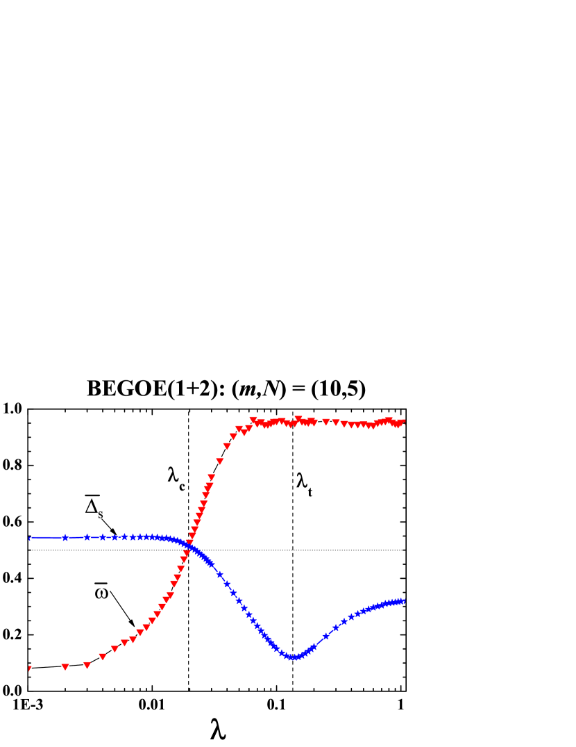
Figure 2: (Color online) Ensemble averaged values $\overline{\omega}$ and $\overline{\Delta_{s}}$ as a function of two body interaction strength $\lambda$, calculated using a 100 member BEGOE(1+2) ensemble with $m=10$ and $N=5$. The vertical dash-lines represent the position of $\lambda_{c}$ and $\lambda_{t}$. Here $\lambda_{c}\simeq 0.02$ and $\lambda_{t}\simeq 0.13$.

IV Duality and $(m,N)$ dependence of $\lambda_{t}$

The duality region $\lambda=\lambda_{d}$ is the point where quantities defining eigenstate properties like entropy, strength functions, temperature etc. give same values irrespective of the defining basis Jacq-02 . Then one can argue that in this region all eigenstates look alike and the duality region defined by $\lambda=\lambda_{d}$ is expected to correspond to the thermodynamic region defined by $\lambda=\lambda_{t}$ as in fermionic EGOE(1+2) results An-04 ; Ma-10 . For the BEGOE(1+2) Hamiltonian, two choices of basis appear naturally. One is mean-field basis defined by $h(1)$ and another is the infinite interaction strength basis defined by $V(2)$. To examine duality, we compare information entropy $S^{info}(E)$ and strength functions $F_{\xi_{k}}(E)$ (also called local density of states (LDOS)) in $h(1)$ basis and in $V(2)$ basis. The strength function corresponding to the $k$’th basis state for a particular member of ensemble is defined by $F_{\xi_{k}}(E)=\sum_{i}|C_{k}^{i}|^{2}\delta(E-E_{i})$, where $k$-energies $\xi_{k}=\langle k|H|k\rangle$ and $|k\rangle$ is the $k$’th basis state for $m$-particles in $N$ sp states. Figure 3 shows numerical results for $S^{info}(E)$ and $F_{\xi_{k}}(E)$ in $h(1)$ and in $V(2)$ basis for a 100 member BEGOE(1+2) ensemble with ($m=10$, $N=5$) for different values of $\lambda$. Here strength functions $F_{\xi_{k}}(E)$ are computed following the procedure described in Ch-04 and results are shown for $\xi_{k}=0$ in the Fig. 3b. It is seen from Fig. 3 that values of $S^{info}(E)$ and $F_{\xi_{k}}(E)$ in these two basis are found very close near $\lambda=0.13$ giving value for the duality marker $\lambda_{d}\simeq 0.13$ for the present example. For $\lambda<\lambda_{d}$, the $S^{info}(E)$ values in the $h(1)$ basis are smaller compared to those in the $V(2)$ basis and for $\lambda>\lambda_{d}$, $S^{info}$ in the $h(1)$ basis is comparatively larger. While opposite behavior is observed from the results of the strength functions. The values of entropy as well as of strength functions in these two basis coincide near $\lambda=\lambda_{d}$. This value is very close to the marker $\lambda_{t}$ and therefore, $\lambda_{d}$ region can be interpreted as the thermodynamic region in the sense that all different definitions of temperature and entropy coincide in this region.

In the $h(1)$ basis, $S^{info}(E)$ is determined using equation given below Ch-03 .

$$\exp[S^{info}(E)-S^{info}_{GOE}]=\sqrt{1-\zeta^{2}}\;\exp\{\frac{\zeta^{2}}{2}\}\;\exp\{-\frac{\zeta^{2}E^{2}}{2}\}\;.$$ (5)

Here $\zeta$ is the correlation coefficient between the full Hamiltonian $H$ and the diagonal part of the full Hamiltonian $H$; it is given by

$$\zeta=\sqrt{1-\frac{\sigma^{2}_{off-diagonal}}{\sigma^{2}_{H}}}=\sqrt{\frac{\sigma^{2}_{h(1)}}{\sigma^{2}_{h(1)}+\lambda^{2}\sigma^{2}_{V(2)}}}\;\;.$$ (6)

We can determine the value of $\lambda_{t}$ by using the condition that $\zeta^{2}=0.5$ An-04 ; i.e. the spreadings produced by $h(1)$ and $V(2)$ are equal at $\lambda_{t}$. In Fig. 4, ensemble averaged values of $\zeta^{2}$ as a function of $\lambda$ for a 100 member BEGOE(1+2) ensemble using ($m,N$)=($10,5$) is presented by filled red circles. It is clear from the figure that for $\lambda\leq\lambda_{c}$, $\zeta^{2}$ is close to $1$ and as $\lambda$ increases, $\zeta^{2}$ goes on decreasing smoothly. The two vertical dash-lines in Fig. 4 indicate the respective positions of $\lambda_{c}$ and $\lambda_{t}$ as obtained in Section III. It can be clearly seen that $\zeta^{2}=0.5$ gives the thermalization point $\lambda_{t}=0.13$. For BEGOE(1+2) ensemble, analytical expression for $\zeta$ based on the method of trace propagation is derived in Ch-04 . With $\zeta^{2}=0.5$ in Eq.(7) of Ch-04 and solving it for $\lambda$, ($m,N$) dependence of marker is given by,

$$\lambda_{t}=2\sqrt{\frac{(N+2)X}{N(N+1)(N-2)(m-1)(N+m+1)}}\;;$$ (7)

where $X=\sum_{i}^{N}{\tilde{\varepsilon_{i}}}^{2}$. For uniform sp spectrum with $\varepsilon_{i}=i$, $X=N(N+1)(N-1)/12$ and $\lambda_{t}=\sqrt{\frac{(N-1)(N+2)}{3(N-2)(m-1)(N+m+1)}}$. With $(m=10,N=5)$, we have $\lambda_{t}\approx 0.15$. For single particle energies which we have used in the present study, $X=N(N^{2}+5)/12$ and

$$\lambda_{t}=\sqrt{\frac{(N+2)(N^{2}+5)}{3(N+1)(N-2)(m-1)(N+m+1)}}\;.$$ (8)

With $(m=10,N=5)$, we have $\lambda_{t}\approx 0.16$. Figure 4 shows plots of $\zeta^{2}$ as a function of $\lambda$ obtained using Eq.(7) of Ch-04 . The blue curve in the figure is obtained due to uniform SPEs while the green curve is obtained due to SPEs employed in the present study. It can be seen from results that the ensemble averaged values are close to the expected values. Small discrepancy is due to the neglect of induced single-particle energies. In the dense limit, Eq.(8) gives $\lambda_{t}\sim\frac{1}{m}\sqrt{\frac{N}{3}}$. Similarly, in the dilute limit, we have $\lambda_{t}\sim\frac{1}{\sqrt{3m}}$ and this result is in agreement with EGOE(1+2) result given in An-04 . From Eq.(8) it is seen that for $m/N$ fixed as $m\rightarrow\infty$ and $N\rightarrow\infty$ (also into strict dense limit), $\lambda_{t}\rightarrow 0$. A similar behavior is expected for $\lambda_{c}$ and $\lambda_{F}$. These sudden transitions with $\lambda>0$ are similar to the situation with Poisson to GOE or GUE KS-1999 ; FGM-1998 and GOE to GUE PM-1983 .

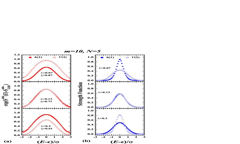
Figure 3: (Color online) Ensembles averaged results for (a) the information entropy and (b) strength functions $F_{\xi_{k}}(E)$ in the $h(1)$ and $V(2)$ basis for a 100 member BEGOE(1+2) ensemble with $(m=10)$ and $(N=5)$ are shown as a function of normalized energy, $(E-\epsilon)/\sigma$, for different $\lambda$ values. Results averaged over bin-size 0.1 are shown as circles; filled circles correspond to $h(1)$ basis and open circles correspond to $V(2)$ basis. Ensemble averaged $\zeta$ values are also given in the figure. Strength function plots are obtained for $\xi_{k}=0$ and in the plots $\int F_{\xi_{k}}(E)dE=1$.

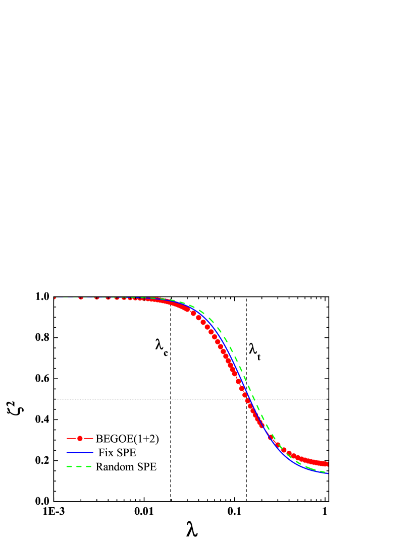
Figure 4: (Color online) Ensemble averaged values of $\zeta^{2}$ (red filled circles) as function of the two-body interaction strength $\lambda$, calculated for a 100 member BEGOE(1+2) ensemble with ($m=10,N=5$) are shown. Smooth curves are obtained using Eq.(7) of ref.Ch-04 . Blue (continuous) curve is for fixed SPEs and green (dash) curve is due to random SPEs used in present study.

V Conclusions

In the present work, we have analyzed the relationship between order to chaos transition and thermalization in finite dense interacting boson systems using one- plus two-body embedded Gaussian orthogonal ensemble of random matrices. Using numerical calculations, it is demonstrated that in a region $\lambda\sim\lambda_{t}$ different definitions give essentially same values for temperature and entropy, thus defining a thermalization region similar to as in fermionic EGOE(1+2) ensembles. The value of $\lambda_{t}$ is much larger than the $\lambda$ value where level fluctuations change from Poisson to GOE and strength functions from Breit-Wigner to Gaussian ($\lambda_{t}>\lambda_{F}>\lambda_{c}$). Further it is established that the duality region where information entropy and strength functions will be the same in both the mean field and interaction defined basis corresponds to a region of thermalization. We have also obtained formula for $\lambda_{t}$ in terms of $(m,N)$. In addition to this, we know that $\lambda_{t}>>\lambda_{c}$, which is further confirmed by the analytical formula for $\lambda_{t}$ given in Eq.(8) and the estimates for $\lambda_{c}$ as given in Ch-03 . Similar results are known for fermion where $\lambda_{c}\propto\frac{1}{m^{2}N}$ and $\lambda_{t}\propto\frac{1}{\sqrt{m}}$. However, for bosons formulas are not available for $\lambda_{c}$ and $\lambda_{F}$. Therefore we cannot tell if $\lambda_{F}$ will be close to $\lambda_{c}$ or $\lambda_{t}$ or it will be far from both. This is an important open problem. The present work brings completion to the study of transition (chaos) markers generated by BEGOE(1+2) initiated in Ch-03 ; Ch-04 . Further investigations on thermalization in BEGOE(1+2) will be discussed in future.

References

- (1) M. Rigol, V. Dunjko, and M. Olshanii, Nature 452 (2008) 854.
- (2) M. Rigol, Phys. Rev. Lett. 103 (2009) 100403; Phys. Rev. A80 (2009) 053607.
- (3) M. Rigol and M. Fitzpatrick, Phys. Rev. A84 (2011) 033640.
- (4) L. F. Santos and M. Rigol, Phys. Rev. E81 (2010) 036206; Phys. Rev. E82 (2010) 031130; M. Rigol and L. F. Santos, Phys. Rev. A82 (2010) 011604(R).
- (5) L. F. Santos, F. Borgonovi, and F. M. Izrailev, Phys. Rev. Lett. 108 (2012) 094102.
- (6) L. F. Santos, F. Borgonovi, and F. M. Izrailev, Phys. Rev. E85 (2012) 036209.
- (7) V. K. B. Kota, A. Relaño, J. Retamosa, and Manan Vyas, J. Stat. Mech. P10028 (2011) 1.
- (8) I. Bloch, J. Dalibard, and W. Zwerger, Rev. Mod. Phys. 80 (2008) 885; S. Trotzky, Yu-Ao Chen, A. Flesch, Ian P. McCulloch, U. Schollw ck, J. Eisert, and I. Bloch, Nature Physics 8 (2012) 325.
- (9) M. Horoi, V. Zelevinsky, and B. A. Brown, Phys. Rev. Lett. 74, (1995) 5194; V. Zelevinsky, B. A. Brown, N. Frazier, and M. Horoi, Phys. Rep. 276 (1996) 85.
- (10) V. K. B. Kota and R. Sahu, Phys. Rev. E66 (2002) 037103.
- (11) G. Benenti, G. Casati, and D. L. Shepelyansky, Euro. Phys. J. D17 (2001) 265.
- (12) M. Žnidarič, T. Prosen, G. Benenti, G. Casati, and D. Rossini, Phys. Rev. E81 (2010) 051135.
- (13) V.K.B. Kota, Phys. Rep. 347 (2001) 223.
- (14) J.M.G. Gómez, K. Kar, V.K.B. Kota, R.A. Molina, A. Relaño, and J. Retamosa , Phys. Rep., 499 (2011) 103.
- (15) V. V. Flambaum, F. M. Izrailev, and G. Casati, Phys. Rev. E54 (1996) 2136; V. V. Flambaum and F. M. Izrailev, Phys. Rev. E56 (1997) 5144.
- (16) V. V. Flambaum and F. M. Izrailev, Phys. Rev. E55 (1997) R13.
- (17) D. Angom, S. Ghosh, and V. K. B. Kota, Phys. Rev. E70 (2004) 016209.
- (18) Manan Vyas, V.K.B. Kota, and N.D. Chavda, Phys. Rev. E81 (2010) 036212(2010).
- (19) V. V. Flambaum and F. M. Izrailev, Phys. Rev. E64 (2001) 036220.
- (20) F. Borgonovi, I. Guarneri, F. M. Izrailev, and G. Casati, Phys. Lett. A247 (1998) 140.
- (21) K. Patel, M.S. Desai, V. Potbhare, and V.K.B. Kota, Phys. Lett. A275 (2000) 329.
- (22) N. D. Chavda, V. Potbhare and V. K. B. Kota, Phys. Lett. A311 (2003) 331.
- (23) N. D. Chavda, V. Potbhare and V. K. B. Kota, Phys. Lett. A326 (2004) 47.
- (24) Manan Vyas, N. D. Chavda, V. K. B. Kota and V. Potbhare, J. Phys. A: Math. Theor. 45 (2012) 265203.
- (25) T. Agasa, L. Benet, T. Rupp, and H. A. Weidenmüller, Eur. Phys. Lett. 56 (2001) 340; T. Agasa, L. Benet, T. Rupp, and H. A. Weidenmüller, Ann. Phys. (N.Y.) 298 (2002) 229.
- (26) V. K. B. Kota and V. Potbhare, Phys. Rev. C21 (1980) 2637.
- (27) R.J. Leclair, R.U. Haq, V.K.B. Kota, and N.D. Chavda, Phys. Lett. A372 (2008) 4373.
- (28) T. A. Brody, J. Flores, J. B. French, P. A. Mello, A. Pandey, and S. S. M. Wong, Rev. Mod. Phys. 53 (1981) 385.
- (29) Ph. Jacquod and I. A. Varga, Phys. Rev. Lett. 89 (2002) 134101.
- (30) V.K.B. Kota, S. Sumedha, Phys. Rev. E60 (1999) 3405.
- (31) K.M. Frahm, T. Guhr, A. Müller-Groeling, Ann. Phys. (N.Y.) 270 (1998) 292.
- (32) A. Pande and M. L. Mehta, Commun. Math. Phys. 87 (1983) 449.