Irrotational, two-dimensional Surface waves in fluids

Abstract

The equations for waves on the surface of an irrotational incompressible fluid are derived in the coordinates of the velocity potential/stream function. The low frequency shallow water approximation for these waves is derived for a varying bottom topography. Most importantly, the conserved norm for the surface waves is derived, important for quantisation of these waves and their use in analog models for black holes.
PACS: 47.90.+a, 92.60.Dj, 04.80.y.

I Introduction

One of the most fascinating predictions of Einstein’s theory of general relativity is the potential existence of black holes – i.e. space-time regions from which nothing is able to escape. Perhaps no less interesting are their antonyms: white holes which nothing can penetrate. Both are described by solutions of the Einstein equations and are related to each other via time-inversion, see e.g. misner ; ellis .

It is equally fascinating that some of the predictions for fields in a black hole spacetime can be modelled by waves in a variety of other situations, with the interior of the black hole or white hole horizons can be mimicked by fluid flow which exceeds the velocity of the waves in some regions. One of these is the use of surface waves on a incompressible fluidschuetz . One can alter the flow properties of the fluid by placing obstacles into the bottom of a flume (a long tank along which the water flows) to speed up and slow down the fluid over these obstacles.

One of the difficulties in the theoretical treatment of such systems is the complicated boundary conditions on the bottom of the tank (where the fluid velocities must be tangential to the bottom) and the top (where the pressure of the fluid must be zero or at a constant atmospheric constant pressure). In fact as we will see the equations for the fluid itself are remarkably simple. The interesting physics arises entirely from those boundary condition.

We will be interested in irrotational, incompressible flow. While both are certainly approximations for water flow (the former assumes no turbulence, and no viscosity which would create vorticity at the shear layer along the bottom, while the latter assumes that the velocity of sound in the fluid is far higher than any other velocities in the problem). While this problem has been investigated beforewaves , this is in general in the three dimensional context (which is more difficult) and using approximations and expansions for the shape of the bottom.

I will assume that the fluid flow is a two dimensional flow– ie is uniform across the tank and that the tank maintains a constant width throughout. This is much simpler case than three dimensional flow, which allows the coordinate transformations I use.

The usual spatial coordinates are $x,y$ with $x$ being the horizontal direction in which the fluid flows, and $y$ is the vertical direction (parallel to the gravitational acceleration, $g$, directed in the negative y direction.

The Euler-Lagrange equations are

$$\partial_{t}\vec{v}+\vec{v}\cdot\nabla\vec{v}=-g\vec{e}_{y}-\vec{\nabla}{p\over\rho}$$ (1)

$$\vec{\nabla}\cdot\vec{v}=0$$ (2)

where the second equation is the incompressibility condition. In the usual way, if we assume that the flow is irrotational, then

$$\vec{v}=\vec{\nabla}\tilde{\phi}$$ (3)

And the above equation can be written as

$$\vec{\nabla}\left(\partial_{t}\tilde{\phi}+{1\over 2}v^{2}+gy+{\tilde{p}\over\rho}\right)=0$$ (4)

$$\nabla^{2}\tilde{\phi}=0$$ (5)

where $\tilde{p}$ is the pressure. Let me define the specific pressure, $p={\tilde{p}\over\rho}$

In the following I will consider only flows in the $x-y$ directions. Everything is assumed to be independent of $z$. Consider the vector $\vec{w}=\vec{e}_{z}\times\vec{v}$. This vector also obeys

$$\nabla\cdot\vec{w}=-\vec{e}_{z}\cdot\vec{\nabla}\times\vec{v}=0$$ (6)

$$\nabla\times\vec{w}=\vec{e}_{z}\vec{\nabla}\cdot\vec{v}-(\vec{e}_{z}\cdot\vec{\nabla})\vec{v}=0$$ (7)

since nothing depends on $z$.

Thus we can define

$$\vec{w}=\vec{\nabla}\tilde{\psi}$$ (8)

where $\tilde{\psi}$ also obeys $\nabla^{2}\tilde{\psi}=0$ and where

$$\nabla\tilde{\psi}\cdot\nabla\tilde{\phi}=0$$ (9)

$$\nabla\tilde{\phi}\cdot\nabla\tilde{\phi}=\vec{v}\cdot\vec{v}=v^{2}$$ (10)

$$\nabla\tilde{\psi}\cdot\nabla\tilde{\psi}=\vec{w}\cdot\vec{w}=v^{2}$$ (11)

Let me now define a new coordinate system. I could use $\tilde{\phi}$ and $\tilde{\psi}$, but I will be interested in fluid flows where the velocity approaches a constant value $v_{x}=v_{0},~{}~{}v_{y}=0$ at large distances. I will thus instead use the functions $\psi,\phi$ defined by

$$\phi={\tilde{\phi}\over v_{0}}$$ (13)

$$\psi={\tilde{\psi}\over v_{0}}$$ (14)

as the new coordinates. This choice will also allow me to take the limit as the velocity $v_{0}$ goes to zero, where the potentials $\tilde{\phi},~{}\tilde{\psi}$ are undefined. Thus at large distances, $\phi=x$ and $\psi=y$. The spatial metric in the $xy$ coordinates is

$$ds^{2}=dx^{2}+dy^{2}=g_{ij}dz^{i}dz^{j}$$ (15)

(where the Einstein summation convention has been used where a repeated index implies summation over that index, and where $z^{1}=x,~{}z^{2}=y$). Do not confuse $z^{i}$ with the horizontal direction $z$ which nothing depends on. The Laplacian is for a general metric function of $g_{ij}(z)$ is

$$\nabla^{2}={1\over\sqrt{|g|}}\partial_{i}\sqrt{|g|}g^{ij}\partial_{j}$$ (16)

where $g^{ij}$ are the components of the matrix with is the inverse to the matrix of coefficients $g_{ij}$ and where $g$ is the determinant of the matrix with coefficients $g_{ij}$. For a reference regarding metrics and the coordinate independent equations see almost any book on General Relativitywald .

In two dimensions, if $g_{ij}=f\tilde{g}_{ij}$ where $f$ is some function of the coordinates $z^{i}$, then since $g^{ij}={1\over f}\tilde{g}^{ij}$ and $g=det(g_{ij})=f^{2}det(\tilde{g}_{ij})=f^{2}\tilde{g}$, we have $\nabla^{2}={1\over f}\tilde{\nabla}^{2}$. Metrics such as $g_{ij}$ and $\tilde{g}_{ij}$ are said to be confomally related.

Recalling that the change in the metric components from one coordinate system $z^{i}$ to a new system $\hat{z}^{j}$ are given by

$$\hat{g}^{kl}={\partial\hat{z}^{K}\over\partial z^{i}}{\partial z^{l}\over\partial z^{j}}g^{ij}$$ (17)

where the Einstein summation convention has been used, the components of the upper components of the usual flat space metric in this new $\hat{z}^{1}=\phi,\hat{z}^{2}=\psi$ coordinate system are

$$\hat{g}^{\phi\phi}=\vec{\nabla}\phi\cdot\vec{\nabla}\phi={v^{2}\over v_{0}^{2}}$$ (18)

$$\hat{g}^{\psi\psi}=\vec{\nabla}\psi\cdot\vec{\nabla}\psi={v^{2}\over v_{0}^{2}}$$ (19)

$$\hat{g}^{\phi\psi}=\vec{\nabla}\phi\cdot\vec{\nabla}\psi=0$$ (20)

Ie, the new metric (the inverse of this upper form metric) in these new coordinates is a conformally flat metric

$$\hat{g}_{ij}={v_{0}^{2}\over v^{2}}\left(\begin{array}[]{ccc}1&0\\ 0&1\end{array}\right)$$ (23)

Since in the $xy$ coordinates the metric is flat, this metric is also flat in $\psi,\phi$ coordinates, (the curvature is not changed by a coordinate transformation) and the scalar curvature in this new coordinate system is zero. Using the equation for the scalar curvature of a metric (and in two dimensions, the scalar curvature is the only independent component of the curvature) one gets

$$(\partial_{\phi}^{2}+\partial_{\psi}^{2})\ln({v^{2}\over v_{0}^{2}})=0$$ (24)

(This is valid as long as $v^{2}\over v_{0}^{2}$ is not equal to zero anywhere)

I define

$$\tilde{\nabla}^{2}=\partial_{\phi}^{2}+\partial_{\psi}^{2}$$ (25)

The Laplacian

$${1\over\sqrt{(}\hat{g})}\partial_{i}\sqrt{\hat{g}}\hat{g}^{ij}\partial_{j}\Phi$$ (26)

is, since the metric in $\psi,\phi$ coordinates is conformally flat, just

$${v^{2}\over v_{0}^{2}}\tilde{\nabla}^{2}\Phi$$ (27)

for any scalar function $\Phi$.

Since in $x,y$ coordinates, the Laplacian of both the scalar functions $x$ and $y$ are zero, they must also be zero in $\phi,\psi$ coordinates ( since the Laplacian is an invariant scalar operator), and, as functions of $\phi,\psi$, we have

$$\tilde{\nabla}^{2}x(\phi,\psi,t)=\tilde{\nabla}^{2}y(\phi,\psi,t)=0$$ (28)

as the equations of motion obeyed by $x$ and $y$ in these new coordinates.

$\psi$ is the stream function, and the vector $\vec{v}$ is tangent to the surfaces of constant $\psi$. $\vec{v}\cdot\vec{\nabla}\psi=\vec{v}\cdot\vec{w}=0$. The bottom of the flow must be tangent to the flow vector (no flow can penetrate the bottom), and thus must be a surface of constant $\psi$, which I will take to be $\psi=0$. Similarly, if the flow is stationary, the top of the water, no matter how convoluted, must also lie along a streamline, since a particle of the fluid which is at the top, must flow along the top (the velocity of the particles must be parallel to the top surface). This means that the top of a stationary flow ( but not a time dependent flow) also is at a constant value of $\psi$ which I will label $\psi_{T}$.

We also have

$$\partial_{x}\phi=\partial_{y}\psi={v_{x}\over v_{0}}$$ (29)

$$\partial_{y}\phi=-\partial_{x}\psi={v_{y}\over v_{0}}\partial_{\phi}x=\partial_{\psi}y={v_{x}v_{0}\over v^{2}}$$ (30)

$$-\partial_{\psi}x=\partial_{\phi}y={v_{y}v_{0}\over v^{2}}$$ (31)

and thus

$${v^{2}\over v_{0}^{2}} = {1\over(\partial_{\phi}y)^{2}+(\partial_{\psi}y)^{2}}$$ (32)

$$= {1\over(\partial_{\phi}x)^{2}+(\partial_{\psi}x)^{2}}$$ (33)

Solving for $x$ and $y$ as a function of $\psi,\phi$ , which is just solving the Laplacian in terms of $\psi,\phi$, gives us the velocity at all points.

The boundary condition along the bottom for these functions must be that the velocity along the bottom be parallel to the bottom. If the bottom has the functional form $y=F(x)$ then $y(\phi,0)=F(x(\phi,0))$. On the top of the flow, we have the boundary condition that $p=0$. From the Bernoulli equation for a stationary flow is

$${1\over 2}v^{2}+gy+p={\rm const}$$ (34)

which, if the flow has constant velocity $u$ over a constant depth bottom of height $h$ far away from the obstacle, gives the equation for the top of the flow

$${1\over 2}v(\phi,\psi_{T})^{2}+gy(\phi,\psi_{T})={1\over 2}v_{0}^{2}+gh$$ (35)

Writing this in terms of $\phi,\psi$ we have the upper boundary condition of

$${v_{0}^{2}\over(2((\partial_{\phi}y(\phi,\psi_{T}))^{2}+(\partial_{\phi}x(\phi,\psi_{T}))^{2}))}+gy(\phi,\psi_{T})={1\over 2}v_{0}^{2}+gh$$ (36)

This is a complicated, non-linear, boundary condition. Thus while the equations of motion of $x,~{}y$ are simple (Laplacian equals zero), the physics is all contained in the boudary conditions.

If we are given $y(x)$ as the equation for the bottom, the solution of the above non-linear boundary value problem is difficult. However if , instead of specifying the lower boundary, one specifies the shape of the upper boundary $y(\phi,\psi_{T})$, one can use Bernoulli’s equation in these new coordinates to determine the $\psi$ derivative of $y$ . Since

$$\partial_{\psi}y={v_{y}\over v^{2}}$$ (37)

$$\partial_{\phi}y={v_{x}\over v^{2}}$$ (38)

we have

$$v^{2}={1\over(\partial_{\psi}y)^{2}+(\partial_{p}hiy)^{2}}$$ (39)

and Bernoulli’s equation is $v^{2}+gy=const$ along the top surface of the fluid where $p=0$. Soving for $\partial_{\psi}y$ we get

$$\partial_{\psi}y(\phi,\psi_{T})=-\sqrt{-((\partial^{\phi}y(\phi,\psi_{T}))^{2}+{1\over v_{0}^{2}+g(y(\infty,\psi_{T})-y(\phi,\psi_{T}))}}$$ (40)

Any function $H(\psi\phi)$ which is a solution of $\partial_{\psi}^{2}H+\partial_{\phi}^{2}H=0$ can be expanded in exponentials $e^{ik\phi}$. We see immediately that the dependence of these modes of $\psi$ must be in terms of $e^{\pm k\psi}$ or equivalently in terms of $cosh(k\psi)$ and $sinh(k\psi)$ for the $\psi$ dependence. Thus, since $y$ obeys that equation, we have

$$y(\phi,\psi)=\int e^{ik\phi}\left(\alpha_{k}\cosh(k(\psi-\psi_{T}))+\beta_{k}\sinh(k(\psi-\psi_{T}))\right)$$ (41)

with

$$\alpha_{k}={1\over 2\pi}\int y(\phi,\phi_{T})e^{-ik\phi}d\phi$$ (42)

$$\beta_{k}={1\over 2\pi}\int{1\over k}\partial_{\psi}y(\phi,\psi_{T})e^{-ik\phi}d\phi$$ (43)

Then at the lower boundary,

$$y(\phi,0)=\int\left[\hat{y}(k){\cosh(k\psi_{T})}-\hat{\partial_{\psi}y}(k){\sinh(k\psi_{T})\over k}\right]e^{ik\phi}dk$$ (44)

$$x(\phi,0)=\int\int\left[\hat{\partial y}(k){k\cosh(k\psi_{T})}+\hat{y}(k){\sinh(k\psi_{T})}\right]e^{ik\phi}dkd\phi$$ (45)

where

$$\hat{y}(k)=\int y(\phi,\psi_{T})e^{-ik\phi}d\phi$$ (46)

$$\hat{\partial y}(k)=\int\partial_{\psi}y(\phi,\psi_{T})e^{-ik\phi}{d\phi}$$ (47)

This gives the bottom as a parametric set of functions of $\phi$.

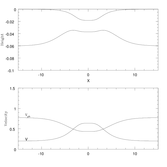
Figure 1: Figure 1. The upper graph gives the top and bottom ($y(\psi_{T})$ and $y(0)$ of a symmetric flume flow with $v_{0}=.3m/s$. The top of the flow was specified with $y(\phi,\psi_{T})=.015(e^{(\psi-.5)^{2}/2}+e^{(\psi+.5)^{2}/2}$. Note that the bottom of the flume is a reasonable function of $x$. The lower graph gives the velocity of the fluid flow, ($v(\phi)$) as a function of $x$ and the phase velocity of long wavelength waves $\sqrt{g(y(\phi,\psi_{T})-y(\phi,0))}$ as a function of $x$. The ratio of these two velocities is the Froude number, which is greater than unity over the obstacle.

In figure 1 we have an example of sub to supercritical flow over an obstacle. calculated as above. Note that the obstacle is a reasonable function $y(x)$.

I.1 $v_{0}=0$ limit

The boundary condition equations are easily solved in the limit as $v_{0}\rightarrow 0$. The upper boundary condition becomes simply $y=h$ and $\partial_{\phi}y=0$. This can be solved (in terms of the unknown lower boundary solutions $y(\phi,0),~{}x(\phi,0)$ by

$$y(\phi,\psi) = \int\alpha_{k}e^{ik\phi}{sinh(k(\psi_{T}-\psi))\over sinh(k\psi_{T})}dk$$ (48)

$$x(\phi,\psi) = i\int\alpha_{k}e^{ik\phi}{cosh(k(\psi_{T}-\psi))\over sinh(k\psi_{T})}dk$$ (49)

where

$$\alpha_{k}={1\over 2\pi}\int y(\phi,0)e^{-ik\phi}d\phi$$ (50)

Of course, we are not given $y(\phi,0)$ but rather $y(\phi,0)=F(x(\phi,0))$. However one can get rapid convergence by iteration

$$x_{0}(\phi,0)=\phi$$ (51)

$$y_{i+1}(\phi,0)=F(x_{i}(\phi,0))$$ (52)

which gives via the above equations the solution $y_{i+1}(\phi,\psi)$ and thus

$$x_{i+1}(\phi,0)=\int\partial_{\psi}y_{i+1}(\phi,0)d\phi$$ (53)

For small $v_{0}$, one can get a first order correction for the surface value of $y(\phi,\psi_{T})$ by taking

$$y(\phi,\psi_{T})=h-v_{0}^{2}{1\over(\partial_{\psi}y_{v_{0}=0}(\phi,\psi))^{2}|_{\psi=\psi_{T}}}$$ (54)

Ie, for slow flow over a bottom boundary, the stationary solution for that flow is easy to find.

I.2 Formal General solution

The general solution to the equation $\tilde{\nabla}^{2}F$=0 can be written as

$$F=f(\phi+i\psi)+g(\phi-i\psi)$$ (55)

If $F$ is real, then $g(\phi-i\psi)=(f(\phi+i\psi))^{*}$ We then have

$$x(\phi,\psi)=\hat{x}(\phi+i\psi)+\hat{x}^{*}(\phi+i\psi)$$ (56)

$$y(\phi,\psi)=i(\hat{x}(\phi+i\psi)-\hat{x}^{*}(\phi+i\psi))$$ (57)

Given the boundary conditions along the bottom, we have

$$\hat{x}(\phi)={1\over 2}(x_{0}(\phi,0)-iy_{0}(\phi,0))$$ (58)

This of course still leaves the highly non-linear boundary conditions at the top to solve to find $x$ and $y$ everywhere.

II Fluctuations

Let us assume that we have a background solution to the stationary equation, $x_{0}(\phi,\psi),y_{0}(\phi,\psi)$, or equivalently, $\phi_{0}(x,y),\psi_{0}(x,y)$. We want to find the equations for small perturbations around this background flow. Let us also consider a solution to the full time dependent equations,$\phi(x,y,t),\psi(x,y,t)$ together with their inverses, $x(\phi,\psi,t),y(\phi,\psi,t)$, such that $y(\phi(x,y,t),\psi(x,y,t),t)=y$ and $x(\phi(x,y,t),\psi(x,y,t),t)=x$. Define the small deviations from the background by

$$\delta\phi = \phi(x,y,t)-\phi_{0}(x,y)$$ (59)

$$\delta\psi = \psi(x,y,t)-\psi_{0}(x,y)$$ (60)

$$\delta x = x(\psi,\phi,t)-x_{0}(\phi,\psi)$$ (61)

$$\delta y = y(\phi,\psi,t)-y_{0}(\phi,\psi)$$ (62)

Then we have

$$y = y(\phi_{0}(x,y)+\delta\phi(x,y,t),\psi_{0}(x,y)+\delta\psi(x,y,t),t)$$ (64)

$$= y_{0}(\phi_{0}(x,y)+\delta\phi(x,y,t),\psi_{0}(x,y)+\delta\psi(x,y,t),t)+\delta y(\phi_{0}(x,y)+\delta\phi(x,y,t),\psi_{0}(x,y)+\delta\psi(x,y,t),t)$$ (65)

Keeping terms only to first order in ”$\delta$”, we have

$$y = y_{0}(\phi_{0}(x,y),\psi_{0}(x,y))+\partial_{\phi}y_{0}(\phi_{0}(x,y),\psi_{0}(x,y))\delta\phi+\partial_{\psi}y_{0}(\phi_{0}(x,y),\psi_{0}(x,y))\delta\psi+\delta y(\phi_{0}(x,y),\psi_{0}(x,y))$$ (66)

or

$$\delta y(\phi_{0}(x,y),\psi_{0}(x,y)) = -{v_{0}v_{y}\over v^{2}}\delta\phi(x,y)-{v_{0}v_{x}\over v^{2}}\delta\psi(x,y)$$ (67)

(where all velocity components are those in the background flow).

Similarly

$$\delta x=-{v_{0}v_{x}\over v^{2}}\delta\phi(x,y)+{v_{0}v_{y}\over v^{2}}\delta\psi(x,y)$$ (68)

and

$$\delta\phi(x_{0}(\phi,\psi),y_{0}(\phi,\psi))={1\over v_{0}}(v_{x}\delta x(\phi,\psi)+v_{y}\delta y(\phi,\psi))$$ (69)

$$\delta\psi(x_{0}(\phi,\psi),y_{0}(\phi,\psi))={1\over v_{0}}(-v_{y}\delta x(\phi,\psi)+v_{x}\delta y(\phi,\psi))$$ (70)

The Bernoulli equation is

$$v_{0}\partial_{t}\phi(x(\phi,\psi,t),y(\phi,\psi,t),t)+{v_{0}^{2}\over 2}{1\over(\partial_{\phi}x(\phi,\psi,t))^{2}+(\partial_{\phi}y(\phi,\psi,t))^{2}}+gy(\phi,\psi,t)+p=const$$ (71)

where the first $\partial_{t}$ is defined as the derivative keeping $x,y$ fixed, not $\phi,\psi$ fixed. Here $p$ is the specific pressure.

Writing this equation perturbatively, we have

$$-v_{x}\partial_{t}\delta x-v_{y}\partial_{t}y-{v_{0}^{2}\over((\partial_{\phi}x)^{2}+(\partial_{\phi}y)^{2})^{2}}\left({v_{0}v_{x}\over v^{2}}\partial_{\phi}\delta x+{v_{0}v_{y}\over v^{2}}\partial_{\phi}y\right)+g\delta y+\delta p=0$$ (72)

where all of the velocities are the values of the background velocities at the location $\phi,\psi$. Ie, $v_{x}(\phi,\psi)=v_{0x}(x_{0}(\phi,\psi),y_{0}(\phi,\psi))$.

We can now rewrite this equation in terms of $\delta\phi=\delta\phi(x_{0}(\phi,\psi),y_{0}(\phi,\psi))$ to get

$$v_{0}\tilde{\partial}_{t}\delta\phi+v^{2}\left(v_{x}\partial_{\phi}({v_{x}\over v^{2}}\delta\phi-{v_{y}\over v^{2}}\delta\psi)+v_{y}(\partial_{\phi}({v_{y}\over v^{2}}\delta\phi+{v_{x}\over v^{2}}\delta\psi)\right)-g({v_{0}v_{x}\over v^{2}}\delta\psi+{v_{0}v_{y}\over v^{2}}\delta\phi+\delta p=0$$ (73)

Recalling that $\partial_{\phi}{v_{x}\over v^{2}}=\partial_{\phi}\partial_{\psi}y_{0}=\partial_{\psi}{v_{0}v_{y}\over v^{2}}$ and $\partial_{\phi}{v_{0}v_{y}\over v^{2}}=-\partial_{\psi}{v_{0}v_{x}\over v^{2}}$, we finally get

$$v_{0}\tilde{\partial}_{t}\delta\phi+v^{2}\partial_{\phi}\delta\phi+\partial_{\phi}({1\over 2}v^{2}+gy_{0})\delta\phi-\partial_{\psi}(gy_{0}+{1\over 2}v^{2})\delta\psi+\delta p=0$$ (74)

The boundary conditions at the bottom are that $\delta x$ and $\delta y$ must be parallel to the bottom, or $v_{x}\delta y-v_{y}\delta x=0$ which is just

$$\delta\psi(\phi,0)=0$$ (75)

At the top, the pressure at the surface must be 0. However the surface is no longer simply $\psi=\psi_{T}$ because of the time dependence of the equations. Let us assume that the surface is defined by

$$\psi=\Psi(\phi,t)+\psi_{T}$$ (76)

Since a particle of the fluid which starts on the surface, remains on the surface, we can define the fluid coordinates $\eta,\zeta$. Then the velocity of the fluid is

$$v^{\phi}={d\over dt}\phi(\zeta,\eta,t)$$ (77)

$$v^{\psi}={d\over dt}\psi(\zeta,\eta,t)$$ (78)

Along the surface, we therefore have

$$v^{\psi}=\partial_{t}\Psi+v^{\phi}\partial_{\phi}\Psi$$ (79)

But,

$$v^{\phi} = {d\over dt}\phi(x(\eta,\zeta,t),y(\eta,\zeta,t),t)$$ (80)

$$= v_{x}\partial_{x}\phi+v_{y}\partial_{y}\phi+\partial_{t}\phi$$ (81)

$$= {v^{2}\over v_{0}}+\partial_{t}\phi(x,y,t)$$ (82)

$$v^{\psi}=\partial_{t}\psi(x,y,t)$$ (83)

Thus, assuming that $\Psi$ is also small (the same order as the other ”$\delta$” terms), we have

$$v_{0}\partial_{t}\Psi+{v^{2}\over v_{0}}\partial_{\phi}\Psi=v_{0}\partial_{t}\delta\psi$$ (84)

On the surface, we have the Bernoulli equation, which to first order is

$${1\over 2}v^{2}(\phi,\psi_{T}+\Psi) + gy_{0}(\phi,\psi_{T}+\Psi)-{1\over 2}v^{2}(\phi,\psi_{T}+\Psi)+gy_{0}(\phi,\psi_{t}+\Psi)+\tilde{\partial}_{t}\delta\phi$$ (85)

$$+ v^{2}\partial_{\phi}\delta\phi-\partial_{\phi}({1\over 2}v^{2}+gy)\delta\phi-\partial_{\psi}({1\over 2}v^{2}+gy)\delta\psi+p-p_{0}=0$$ (86)

But along the surface $\psi=\psi_{T}$, the background ${1\over 2}v^{2}+gy$ is constant, so the $\phi$ derivative is 0. We have

$$(\tilde{\partial}_{t}+v^{2}\partial_{\phi})\delta\phi+\partial_{\psi}({1\over 2}v^{2}+gy)(\Psi-\delta\psi)=0$$ (87)

Dividing by $G=\partial_{\psi}({1\over 2}v^{2}+gy)$ and taking the derivative $\tilde{\partial}_{t}+{v^{2}\over v_{0}}\partial_{\phi}$ we get

$$(\tilde{\partial}_{t}+{v^{2}\over v_{0}}\partial_{\phi})\left[{1\over G}(\tilde{\partial}_{t}+{v^{2}\over v_{0}}\partial_{\phi})\right]\delta\phi-{v^{2}\over v_{0}}\partial_{\phi}\delta\psi=0$$ (88)

as the equation of motion for the surface wave. $\delta\phi$ and $\delta\psi$ are related by the boundary condition $\delta\phi=0$ along the bottom.

Since both $\delta\phi$ and $\delta\psi$ obey $\nabla^{2}\delta\psi=\nabla^{2}\delta\phi=0$, we have

$$\tilde{\nabla}^{2}\delta\psi=\tilde{\nabla}^{2}\delta\phi=0$$ (89)

Furthermore, since

$$\partial_{x}\delta\phi=\partial_{y}\delta\psi$$ (90)

$$\partial_{y}\delta\phi=-\partial_{x}\delta\psi$$ (91)

so

$$\partial_{\phi}\delta\phi = \partial_{\phi}x_{0}\partial_{x}\delta\phi+\partial_{\phi}y_{0}\partial_{y}\delta\phi\phi$$ (92)

$$= \partial_{\psi}y_{0}\partial_{y}\delta\psi-\partial_{\psi}x_{0}(-\partial_{x}\delta\psi)=\partial_{\psi}\delta\psi$$ (93)

$$\partial_{\psi}\delta\phi = -\partial_{\phi}\delta\psi$$ (94)

For irrotational time-independent flow, the acceleration of a parcel of fluid is $\vec{v}\cdot\nabla\vec{v}=\vec{\nabla}({1\over 2}v^{2})$ and the orthogonal component of this, the centripetal acceleration is

$${1\over|\nabla\psi|^{2}}\nabla\psi\cdot\nabla({1\over 2}v^{2}={1\over v}\partial_{\psi}({1\over 2}v^{2})$$ (95)

Also $g\partial_{\psi}y=g{v_{x}v_{0}\over v^{2}}\approx gv_{0}/v$ so$Gv/v_{0}$ is the effective gravitational field orthogonal to the flow lines (including the centripital acceleration) .

However it is important to note that it is the effective force of gravity only at the surface of the fluid, not at the obstacle to the flow along the bottom, that is important for the equations of motion.

III Shallow water waves

Since $\phi,~{}\psi$ are real functions, the solutions can be written as

$$\delta\phi(\phi,\psi)=Z(\phi+i\psi)+(Z(\phi+i\psi))^{*}$$ (96)

$$\delta\psi(\phi,\psi)=i(Z(\phi+i\psi)-(Z(\phi+i\psi))^{*})$$ (97)

for some function $Z$. These functions clearly satisfy the Laplacian equation for, and furthermore also satisfy the differential relations on the derivatives of $x,y$ with respect to $\phi,psi$ This gives

$$0=\delta\psi(\phi,0)=i(Z(\phi)-Z^{*}(\phi))$$ (98)

Ie, $Z$ is a real function of a real arguments. which gives

$$\delta\phi(\phi,\psi)=(Z(\phi+i\psi)+Z(\phi-i\psi))\approx 2Z(\phi)+Z^{\prime\prime}(\phi)\psi^{2}$$ (99)

$$\delta\psi=2\psi Z^{\prime}(\phi)$$ (100)

or, to first order in $\psi_{T}$

$$\delta\psi=\psi_{T}\partial_{\phi}\delta\phi$$ (101)

The equation for the waves then becomes

$$(\tilde{\partial}_{t}+v^{2}\partial_{\phi}){1\over G}(\tilde{\partial}_{t}+v^{2}\partial_{\phi})\delta\phi-v^{2}\psi_{T}\partial_{\phi}^{2}\delta\phi=0$$ (102)

We note that this is not a Hermitian operator acting on $\delta\phi$. Recall that a Hermitian operator is one such that

$$\int\delta\hat{\phi}{\cal H}\phi d\phi dt=\int({\cal H}\delta\hat{\phi})\delta\phi d\phi dt$$ (103)

if we assume that all of the boundary terms in the integration by parts are zero. We can rewrite the equation for $\delta\phi$ by dividing by $v^{2}$ as

$$(\tilde{\partial}_{t}+\partial_{\phi}v^{2}){1\over v^{2}G}(\tilde{\partial}_{t}+v^{2}\partial_{\phi})\delta\phi-\psi_{T}\partial_{\phi}^{2}\delta\phi=0$$ (104)

This is a symmetric equation, derivable from an action,

$$\int\left[{1\over v^{2}G}(\tilde{\partial}_{t}+v^{2}\partial_{\phi})\delta\phi^{*}(\tilde{\partial}_{t}+v^{2}\partial_{\phi})\delta\phi-\Psi_{T}\partial_{\phi}\delta\phi^{*}\partial_{\phi}\delta\phi\right]d\phi dt$$ (105)

This action has the global symmetry $\delta\phi\rightarrow e^{i\mu}\delta\phi$ and thus has the usual Noether current associated with this symmetry. In particular it has the conserved norm

$$<\delta\phi,\delta\phi^{\prime}>={i\over 2}\int\left\{\delta\phi^{*}{1\over Gv}(\partial_{t}+v^{2}\partial_{\phi}){\delta\phi^{\prime}\over v}-\delta\phi^{\prime}{1\over Gv}(\partial_{t}+v^{2}\partial_{\phi}){\delta\phi^{*}\over v}\right\}d\phi$$ (106)

IV Deep Water waves

For deep water waves, we can assume that either $Z(\phi+i\psi_{T})>>Z(\psi-i\phi_{T})$ or $Z(\phi+i\psi_{T})<<Z(\psi-i\phi_{T})$. (ie, we assume that as analytic functions, $Z$ goes to zero either in the upper or lower half plane.)

Let us also assume it is the first case, and let us define $\hat{Z}(\phi)=Z(\phi+i\psi_{T})$, and that $\tilde{\partial}_{t}\delta\phi=i\omega\delta\phi$ We then have

$$(i\omega+v^{2}\partial_{\phi}){1\over G}(i\omega+v^{2}_{\phi})]\hat{Z}-(-i)v^{2}\partial_{\phi}\hat{Z}=0$$ (107)

If we assume that $K=i(\partial_{\phi}ln(\hat{Z}))$ is large and negative, such that $\hat{Z}$ varies faster than $v^{2}$ or $G$, we have approximately

$${(\omega+v^{2}(\phi)K)^{2}\over G}+Kv^{2}=0$$ (108)

or

$$\omega=-v^{2}K\pm\sqrt{v^{2}GK}$$ (109)

V General Linearized waves

The equation in general is

$$(\tilde{\partial}_{t}+v^{2}\partial_{\phi}){1\over G}(\tilde{\partial}_{t}+v^{2}\partial_{\phi})\delta\phi-v^{2}\partial_{\phi}\delta\psi=0$$ (110)

Fourier transforming with respect to $\phi$ and $\psi$, and using the fact that $\delta\psi=0$ at $\psi=0$, the functions $\delta\phi,\delta\psi$ then can be written as

$$\delta\phi(\phi,\psi,t)=\int A(k,t)e^{ik\phi}\cosh(k\psi)dk$$ (111)

$$\delta\psi(\phi,\psi,t)=i\int A(k,t)e^{ik\phi}\sinh(k\psi)dk$$ (112)

since again they obey the Laplacian equal to zero in these variables.

Defining $B(k,t)=A(k,t)cosh(k\psi)$ this can be written as

$$\delta\phi(\phi,\psi_{T},t) = \int B(k,t)e^{ik\phi}dk$$ (113)

$$\delta\psi(\phi,\psi_{T},t) = i\int B(k,t)e^{ik\phi_{T}}\tanh(k\psi)dk=i\tanh(-i\psi_{T}\partial_{\phi})\int B(k,t)e^{ik\phi}dk=i\tanh(-i\psi_{T}\partial_{\phi})\delta\phi$$ (114)

Thus the equation of the surface waves can be written as

$$0 = (\tilde{\partial}_{t}+\partial_{\phi}v^{2}){1\over v^{2}G}(\tilde{\partial}_{t}+v^{2}\partial_{\phi})\delta\phi-i\partial_{k}\tanh(-i\psi_{T}\partial_{\phi})\delta\phi$$ (115)

Ie, we get the usual $\tanh$ dispersion relation for the transition from shallow to deep water waves.

This equation is symmetric and real, and thus if $\delta\phi$ is a solution, so is $\delta\phi^{*}$. Again this gives a conserved norm between two solutions to the equations of motion $\delta\phi$ and $\delta\phi^{\prime}$ of

$$<\delta\phi,\delta\phi^{\prime}>=\int{1\over v^{2}G}\left[\phi^{*}(\tilde{\partial}_{t}+v^{2}\partial_{\phi})\delta\phi^{\prime}-\delta\phi^{\prime}(\tilde{\partial}_{t}+v^{2}\partial_{\phi}){\delta\phi}^{*}\right]d\phi$$ (116)

We note that this equation depends only the conditions at the surface of the flow. It is defined entirely in terms of the factors ($v^{2}$ and $G=\partial_{\psi}(gy+{1\over 2}v^{2}$) defined at $\psi=\psi_{T}$, and is independent of the obstacles, or the flow throughout the rest of the stream except insofar as they affect the flow at the surface. This might well change if either vorticity or viscosity were introduced into the equations.

This norm is crucial to the analysis of the wave equation. It is conserved (in the absence of viscosity), and in the use of such waves as models for black holes, it is this norm which determines the Bugoliubov coefficients (or the amplification factor) for waves in the vicinity of a horizon (blocking flow in the hydrodynamics sense) and determines the quantum noise (Hawking radiation) emitted by such a horizon analog. The quantum norm used in the quantization procedure is

$$\langle\delta\phi,\delta\phi\rangle_{Q}={i\over 2}<\delta\phi,\delta\phi>$$ (117)

If we define a new coordinate $\hat{\phi}=\int{1\over v^{2}}d\phi$, the norm becomes

$$<\delta\phi,\delta\phi^{\prime}>=\int({1\over G}\left[\delta\phi^{*}(\tilde{\partial}_{t}-\partial_{\hat{\psi}})\delta\phi^{\prime}-\delta\phi^{*}(\tilde{\partial}_{t}-\partial_{\hat{\psi}})\delta\phi\right]d\hat{\phi}$$ (118)

If the surface of the flow is shallow (${dy_{T}\over dx}<<1$) then ${d\phi\over dx}=v_{x}\approx v$ and $\hat{\phi}\approx{dx\over v_{x}}$.

To relate this to the measured quantity, the vertical displacement at the surface of the waves, we must relate $\delta\phi$ to $\delta y$ at the surface of the fluid. We have

$$\Psi(t,\phi)=\psi(t,x,y_{T}(t,x))-\psi_{T}=\delta\psi(t,x(\phi,\psi_{T}),y(\phi,\psi_{T})+v_{x}\delta y_{T}$$ (119)

or

$$\delta y_{T}={1\over v_{x}}(\Psi-\delta\psi)={1\over Gv_{x}}\partial_{t}+v^{2}\partial_{\phi})\delta\phi$$ (120)

Now, $Gv_{x}\approx g{v_{x}^{2}\over v^{2}}\approx g$ (ignoring the centrifugal contribution to the effective gravity), so the norm becomes

$$<\delta y_{t},\delta y_{T}> = \int{v^{2}\over g}\left[(\partial_{t}+\partial_{\hat{\psi}})^{-1}\delta y_{T}^{*}\delta y_{T}-(\partial_{t}+\partial_{\hat{\psi}})^{-1}\delta y_{T}\delta y_{T}^{*}\right]d\hat{\phi}$$ (121)

$$= \int{1\over g}\left[((\partial_{t}+\partial_{\hat{\psi}})^{-1}\sqrt{v}\delta y_{T}^{*})\sqrt{v}\delta y_{T}-((\partial_{t}+\partial_{\hat{\psi}})^{-1}\sqrt{v}\delta y_{T})\sqrt{v}\delta y_{T}^{*}\right]d\hat{\phi}$$ (122)

and $d{\hat{\phi}}{d\phi\over v^{2}}\approx{dx\over v}$

If we assume that the incoming wave is at a set frequency $\omega$ and take the fourier transform with respect to $t,\hat{x}$ of $\sqrt{v(\hat{\psi})}y_{T}(t,\hat{\phi})$ this becomes

$$<\delta y,\delta y>=\int{|(\sqrt{v}y_{T})(\hat{k})|^{2}\over(\omega+\hat{k})}d\hat{k}$$ (123)

We can also look at the norm current.

$$\partial_{t}\int_{\phi_{1}}^{\phi_{2}}{1\over v^{2}G}\left[\phi^{*}(\tilde{\partial}_{t}+v^{2}\partial_{\phi})\delta\phi^{\prime}-\delta\phi^{\prime}(\tilde{\partial}_{t}+v^{2}\partial_{\phi}){\delta\phi}^{*}\right]d\phi$$ (124)

$$~{}=\int_{\phi_{1}}^{\phi_{2}}\partial_{x}({1\over G}(\tilde{\partial}_{t}+v^{2}\partial_{\phi}^{*})\delta\phi-\partial_{x}({1\over G}(\tilde{\partial}_{t}+v^{2}\partial_{\phi})\delta\phi^{*})+\left[(-i\partial_{\phi}\tanh(-i\psi_{T}\partial_{\phi})\delta\phi^{*})\delta\phi-(i\partial_{\phi}\tanh(i\psi_{T})\partial_{\phi})\delta\phi^{*})\delta\phi\right]d\phi$$

The integrand is a complete derivatives. Although this is not obvious for the terms with the $\tanh$ in them, we can use

$$(\partial_{\phi}^{2n}\delta\phi^{*})\delta\phi-\delta\phi^{*}\partial_{\phi}^{2n}\delta\phi=\partial_{\phi}(\sum_{r=0}^{2n-1}(-1)^{r}\partial_{\phi}^{r}\delta\phi^{*r}\partial_{\phi}^{2n-1-r}\delta\phi)$$ (125)

and the fact that $i\partial_{\phi}\tanh(i\psi_{T}\partial_{\phi})$ can be expanded in a power series in $\partial_{\phi}^{2}$ to show that they also a complete derivative..

Thus the integrand can be written in terms of a complete derivative of with respect to $\partial_{\psi}$ and we can regard the term that is being taken the derivative of as a spatial norm current $J^{\phi}$ so that if $J^{t}$ is the temporal part of the norm current, we have $\partial_{t}J^{t}+\partial_{\phi}J^{\phi}=0$.

If we are in a regime where $\delta\phi=Ae^{-i\omega t-k\phi}$, (ie, a regime where the velocity $v$ and $G$ are both constants), then we have

$$J^{\phi}=i|A|^{2}{(\omega+v^{2}k)\over Gv^{2}}+\partial_{k}(k\tanh(\Psi_{T}k))=i|A|^{2}\omega{(1+v^{2}/v_{p}-2v_{g})\over Gv^{2}}$$ (126)

where $v_{p}$ and $v_{g}$ are the phase and group velocity of the wave. In a situation in which one has a wave train with some definite frequency and wave number entering a region, then the sum of all the norm currents for each $k$ at the boundary of the region must be zero.

VI Blocking flow

Let us return to the static situation. Define $U=\partial_{\phi}\delta\phi$, we have the equation

$$\partial_{\phi}{v^{2}\over G}U+i\tanh(i\psi_{T}\partial_{\phi})U=0$$ (127)

As above, there is a solution if we assume that the derivatives are small, which gives

$$U={{\rm const}\over{v^{2}\over G}-\psi_{T}}$$ (128)

For rapid variations, we have

$$U={\rm const}{v^{2}\over G}e^{i\int{G\over v^{2}}d\phi}$$ (129)

with the transition from one to the other occuring roughly when the logarithmic derivatives of the two solutions are equal

$${(v^{2}/G)^{\prime}\over{v^{2}\over G}-\psi_{T}}\approx{\sqrt{{(v^{2}/G)^{\prime}}^{2}+1}\over v^{2}/G}$$ (130)

Defining the Froude number by $F^{2}={v^{2}\over G\psi_{T}}$ (the square of the velocity of the fluid over the velocity of the long wavelengths in the fluid in the WKB approximation), we have

$${(F^{2})^{\prime}\over F^{2}-1}\approx\sqrt{4(\ln(F)^{\prime})^{2}+\left({1\over F^{2}\psi_{T}}\right)^{2}}$$ (132)

Note that for a non-trivial rate of change of of the bottom, the turning point occurs well before the horizon.

The ^′ denotes derivative with respect to $\phi$ not x. We can rewrite this approximately (assuming that ${v_{x}\over v}\approx 1$ and that $2ln(F)^{\prime}<1\over F^{2}\psi_{T}$ and $\psi_{T}\approx vd$ where d is the depth of the water at postion $x$. as

$${dF^{2}\over dx}\approx{(F^{2}-1)\over F^{2}d}$$ (133)

Note that this transition occurs before $G\psi_{T}=v^{2}$ or Froude number equals 1. The wave on the slope piles up and its frequency makes the transition to deep water wave before we hit the effective horizon.

The long wavelength equation,

$${1\over v^{2}}(\tilde{\partial}_{t}+v^{2}\partial_{\phi}){1\over G}(\tilde{\partial}_{t}+v^{2}\partial_{\phi})\delta\phi-\psi_{T}\partial_{\phi}^{2}\delta\phi=0$$ (134)

is not that of a two dimension metric, which is always conformally flat, but can be written as a the wave equation for a three dimensional metric where all derivatives are equal to zero in the third $\xi$ dimension for the variable $\delta\phi$. The metric is

$$ds^{2}=\alpha((1-{v^{2}\over G\psi_{T}})dt^{2}+2{1\over G\psi_{T}}dtd\phi-{1\over v^{2}G\psi_{T}}d\phi^{2})-{1\over v^{2}G\psi_{T}}d\xi^{2}$$ (135)

where $\alpha$ is an arbitrary function of $\phi$, a two dimensional conformal factor which does not affect the two dimensional wave equation This metric has surface gravity

$$\kappa={v^{2}\over 2}\partial_{\phi}\left(({v^{2}\over G\psi_{T}})\right)={1\over 2}v^{2}\partial_{\phi}F^{2}$$ (136)

(The surface gravity is the acceleration in the metric as seen from far away. for a static time independent metric in a coordinate system which is regular across the horizon, it can be defined by $\kappa=\Gamma^{t}_{tt}$ at the horizon, where $\Gamma^{i}_{jk}$ is the Christofell symbol for the metric. Then $\Gamma^{t}_{tt}=-{1\over 2}g^{t\phi}(\partial_{\phi}g_{tt})$ at the horizon.)

VII Conversion to $\delta y$

Of course $\delta\phi$ is not what is actually measured in an experiment. That is the fluctuation $\Delta y(x)$ which is the difference in height between the stationary flow, and the height with the wave present. We can relate this to $\delta\psi$ and $\Psi$.

$$y_{s}(x,t)=y_{0}(x)+\Delta y(x,t)$$ (137)

where $y_{0}$ is the surface for the background.

$$\delta y={v_{y}\over v^{2}}\delta\phi+{v_{x}\over v^{2}}\delta\psi$$ (138)

Since $\delta\psi=\tanh(\Psi_{H}\partial_{\phi})\delta\phi$, we have

$$v^{2}\delta y=[v_{y}+v_{x}\tanh(\Psi_{H}\partial_{\phi}))]\delta\phi$$ (139)

Inverting this for deep water waves,

$$\delta\phi={v^{2}\over v_{y}+v_{x}}\delta y$$ (140)

while for shallow water waves

$$\delta\phi=\int exp^{-\int{v_{y}\over v_{x}}d\phi}{v^{2}\over v_{x}}\delta yd\phi$$ (141)

The integrand in the exponent is non-zero only in the region where the background flow is dimpled, and, since $v_{y}\over v_{x}$ is in general very small, the exponential can be neglected in most situations.

In the intermediate region, where the wave changes from shallow to deep water wave, there is no easy solution to these equations, but they can be integrated numerically.

VIII Waves in stationary water over uneven bottom

In the limit as $v_{0}$ goes to zero, so does $v$ with the ratio being a finite function. $y$ obeys the equation $\partial_{\phi}^{2}+\partial_{\psi}^{2}y=0$ with the boundary conditions along the bottom that $y=Y(x)$, with Y the given function of x of the bottom, and along the top, $y=H$, a constant. If we assume that we know $Y(\phi)$ (instead of $Y(x)$) along the bottom, this can be solved by

$$y(\phi,\psi)=H+\int\alpha(k)e^{ik\phi}{sinh(k(\psi-\psi_{T}))\over sinh(k\psi_{T})}dk$$ (142)

where

$$\alpha(k)={1\over 2\pi}\int Y(\phi)e^{ik\phi}$$ (143)

and

$$x(\phi,\psi)=\phi+i\int\alpha(k){cosh(k(\psi-\psi_{T}))\over sinh(k(\psi_{T}))}dk$$ (144)

One gets rapid convergence if one starts by taking $x=\phi$, substituting into $Y(x(\phi))$ to find $Y(\phi)$, finding the new $x(\phi)$ and substituting in again.

Then $v_{y}\over v_{0}$ at the surface is zero, while

$${v_{0}\over v_{x}}={v_{0}\over v}=\partial_{\psi}y=\int k\alpha(k){1\over sinh(k(\psi_{T}))}dk$$ (145)

The equation for small perturbations becomes

$${v_{0}^{2}\over v^{2}G}\partial_{t}^{2}\delta\phi-i\partial_{\phi}\tanh(i\psi_{T}\partial_{\phi})\delta\phi=0$$ (146)

where

$${v^{2}\over v_{0}^{2}}G={v^{2}\over v_{0}^{2}}g\partial_{\psi}y=g{v_{x}\over v_{0}}=g{\partial\phi\over\partial_{x}}$$ (147)

.If the depth is constant, the backgound $\psi=y$ and $\phi=x$ giving the usual equation, which allows us to write

$$\partial_{t}^{2}\delta\phi+ig\partial_{x}\tanh(\psi_{T}\partial_{\phi})\delta\phi$$ (148)

For deep water waves, where the $\tanh$ is unity, this equation is exactly the same as the deep water equation for constant depth. The fact that the bottom varies makes no difference to the propagation of the waves, as one would expect.

For shallow water waves, where the $\tanh$ can be approximated as the linear function in its argument, the equation becomes

$$\partial_{t}^{2}\delta\phi=\psi_{T}\partial_{x}\partial_{\phi}\delta\psi=g\psi_{T}{v_{0}\over v}\partial_{x}^{2}\delta\phi$$ (149)

This allows us to determine the wave propagation over an arbitrarily defined bottom. Note that in the stationary limit, the background flow is certainly irrotational, implying that the assumptions made here should certainly be valid (of course neglecting the viscosity of the fluid).

Acknowledgement This work was supported by The Canadian Institute for Advanced Research (CIfAR) and by The Natureal Science and Engineering Research Council of Canada (NSERC) and was completed while the author was a visitor at the Perimeter Institute.

References

• (1) C. M. Misner, K. S. Thorne, and J. A. Wheeler, Gravitation, (Freemann, San Francisco, 1973).
• (2) S. W. Hawking and G. F. R. Ellis, The Large Scale Structure of Space-time, (Cambridge University Press, Cambridge, England, 1973);
• (3) ¨ R. Schützhold and W. G. Unruh, Phys. Rev. D 66, 044019 (2002).
• (4) Joseph B. Keller ”Surface waves on water of non-uniform depth” J. fluid Mech. 4 607; J.C.W Birkoff ”Computation of combined refraction-diffraction” Proceedings 13th International Conference on Coastal Engineering, Vancouver, ed. G. D. Khaskhachikh, M. . Plakida, I. Ya. Popov pp. 471, Springer (1972)
• (5) R.M. Wald ”General Relativity” U. Chicago Press (1984)
• (6) http://en.wikipedia.org/wiki/Mild-slope_equation (retrieved Oct 10,2011)