A model for stable interfacial crack growth

Abstract

We present a model for stable crack growth in a constrained geometry. The morphology of such cracks show scaling properties consistent with self affinity. Recent experiments show that there are two distinct self-affine regimes, one on small scales whereas the other at large scales. It is believed that two different physical mechanisms are responsible for this. The model we introduce aims to investigate the two mechanisms in a single system. We do find two distinct scaling regimes in the model.

1 Introduction

On a fine enough scale, fractures are rough. How to describe this roughness quantitatively? An answer to this question was first proposed by Mandelbrot et al. in 1984 [1]: Fractures are fractal and their morphology may be described quantitatively by a fractal dimension. In 1990 Bouchaud et al. [2, 3], using the more precise concept of self-affinity rather than fractality to characterize the fracture morphology of metals, proposed that the scaling properties are universal, i.e., they do not depend on the material that fractures. An important conceptual step forwards was taken by Bouchaud et al. [4] when they regarded the fracture surface to represent a “footprint” of a passing fluctuating line, the crack front. Schmittbuhl et al. [5] then made the suggestion that one may simplify the problem by constraining the crack growth to appear between two sintered plates and then follow the fluctuations of the crack front as it moves when the two plates are plied apart as show in Figure 1. In 1997, Schmittbuhl and Måløy [6] realized this system experimentally by sintering two sandblasted plexiglass plates together.

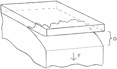
Figure 1: Sketch of the system we model. The two external control parameters are $F$ and $D$, representing either force-controlled or displacement-controlled loading, respectively.

Schmittbuhl et al. [5] presented a numerical model for constrained crack growth based on the fluctuating line picture. Here an elastic line moves through a plane covered with pinning centers. The elastic forces that the line feels is transmitted through the media constituting the two sintered plates. Their main result was to determine the roughness exponent of the self-affine fracture front. If the front is given by $h=h(x)$, where the $x$-direction is orthogonal to the crack growth direction, then self affinity manifests itself through the following invariance: If $p(h,x)$ is the probability density that the crack is at height $h$ at $x$ when it is $h=0$ at $x=0$, then we have

$$\lambda^{\zeta}\ p(\lambda^{\zeta}h,\lambda x)=p(h,x)\;,$$ (1)

where $\zeta$ is the Hurst or roughness exponent. Schmittbuhl et al. [5] found $\zeta=0.35$. This value was later refined to $\zeta=0.39$ by Rosso and Krauth [7]. The experiments [6], on the other hand, gave a much larger roughness exponent, $\zeta=0.55\pm 0.05$. In 2003, Schmittbuhl et al. [8] proposed a model based on the crack front propagating due to coalescence of damage appearing in front of it. This model gave a roughness exponent $\zeta=0.60\pm 0.05$. Recently, Santucci et al. [9] have analyzed larger experimental systems than had been considered earlier. They find a crossover between two scaling regimes in their data; a small-scale regime where $\zeta_{1}=0.60\pm 0.05$ and a large-scale regime where $\zeta_{2}=0.35\pm 0.05$. Combining this result with the previous mechanism that has been suggested — a fluctuating elastic line — it is tempting to propose that the fracture coalescence mechanisms is at work on small scales, whereas on larger scales, the system effectively behaves as the fluctuating line model indicates.

It is the aim of this project to construct a single model capable of capturing both mechanisms and then to study the crossover between them. In the next section, we present the model, which is a variant of the fiber bundle model [10, 11]. The aim of this paper is to present this model in detail, including the computational side, which will be covered in Section 3. We present the treadmill technique in Section 4, which allows us to maintain a stable crack growth. In Section 5 we present our results, two different roughness exponents $\zeta_{1}=0.45$ and $\zeta_{2}=0.3$. These values are low in comparison with the experimental values, $\zeta_{1}=0.60$ and $\zeta_{2}=0.3$. As we will argue, this is probably due to the limited system sizes we so far have considered.

2 The model

Our model is based on an idea originally proposed by Batrouni et al. [10], but with some significant alterations. The basis of the model is a variation of the fiber bundle model, in which linear elastic fibers stretch according to the difference between their local displacement $u_{i}$ and a global displacement $D$,

$$f_{i}=-k_{i}(u_{i}-D).$$ (2)

This relation contains the proportionality constant $k_{i}$, which defines the response of the fiber. $L\times L$ fibers are arranged in parallel, with each fiber connected to two elastic blocks. Each block behaves linearly elastic and can have its own elastic constant, but for simplicity and without loss of generality, one of the regions is set infinitely stiff and the other one elastic with Young’s modulus $E$. The response of the fibers are transmitted through the elastic region via the Green’s function [12],

$$u_{i} =\sum_{j}G_{ij}f_{i},$$ (3a)

$$G_{ij}=\frac{1-\nu^{2}}{\pi Ea^{2}} \iint^{a/2}_{-a/2}\frac{dx^{\prime}dy^{\prime}}{|\vec{r}_{i}(x,y)-\vec{r}_{j}(x^{\prime},y^{\prime})|}.$$ (3b)

where $\nu$ is the Poisson ratio and $a^{2}$ is the area the force of each fiber acts on, thus giving the discretization of the system. $\vec{r}_{i}-\vec{r}_{j}$ gives the distance between fiber $i$ and $j$. The two regions are pulled apart either by controlling an external force or the displacement between them, as shown in Figure 1. The fibers break when they are stretched beyond a given threshold distribution. In matrix notation, the problem can be re-written as

$$(\mathbb{I}+\mathbb{KG})\vec{f}=\mathbb{K}\vec{D},$$ (4)

where $\mathbb{K}$ is an $L^{2}\times L^{2}$ diagonal matrix where $\mathbb{K}_{ii}=k_{i}$. To simplify the problem we keep all constants equal to unity. This is to isolate the disorder in the system to the thresholds, thus avoiding the complications of simultaneously dealing with two quenched disorder distributions. Because of the $1/r$-dependence in the Green’s function (3), there are long-reaching forces in the system and every fiber is connected to every other fiber through the Green’s function, making $\mathbb{G}$ a dense $L^{2}\times L^{2}$ matrix. $\mathbb{I}$ is the identity matrix and we have chosen to give the displacement vector $\vec{D}$ and solve for the forces in the $L^{2}$ vector $\vec{f}$.

We implement our model on a square lattice using bi-periodic boundary conditions with respect to the transmission of the forces. Such boundary conditions are necessary due to numerical effects that we detail in the following. We solve the matrix equation (4) and locate the fiber with the highest ratio of strain to threshold. Then we break that fiber $i$ by setting $k_{i}$ to zero, indicating that it no longer has any load-bearing capability. The process is repeated until all fibers are broken.

2.1 Loading schemes

One of the new concepts of our model is the way we load our system. Providing a uniform displacement vector amounts to pulling the system apart, keeping the two surfaces parallel. Our main goal using this model was to observe a fracture front, meaning that we need some sort of gradient in the system to emulate the loading conditions of the experiments of Schmittbuhl and Måløy [6]. There are at least three ways this can be done. The gradient can either be in the force, the displacement, or the thresholds.

Implementing a gradient in the force applied to the system would amount to solving the inverse problem since the system now would be load controlled. This is only possible by either reformulating the problem or adding a matrix inversion per broken fiber in a simulation, which would be very computationally costly. Given a choice between the displacement and the thresholds, choosing the thresholds enables us compare our results to that of gradient percolation which then would be an extreme limit of the system where it is the treshold distribution that completely dominate how the breakdown process proceeds rather than the force distribution of the fibers. Implementing a linear gradient in the thresholds models the pulling apart of the two blocks at a constant contact angle. This simplifies the problem and maintains a close approximation to realistic loading.

3 Numerical procedures

We use the conjugate gradient (CG) algorithm with Fourier acceleration [10, 14] of the matrix multiplications to solve the system, meaning that the complete system we solve is

$$(\mathbb{I}+\mathbb{KF}^{-1}\mathbb{F}^{1}\mathbb{G})\mathbb{F}^{-1}\mathbb{F}^{1}\vec{f}=\mathbb{K}\vec{D}.$$ (5)

The choice of an iterative solver is due to the matrix $\mathbb{KG}$ evolving from dense to sparse as the simulation progresses. We can Fourier accelerate because the Green’s function, which in essence is a two-point correlation function, is only dependent on the distance between the points in question. This property makes the matrix $\mathbb{G}$ diagonal in Fourier space. Exploiting this, along with the symmetric properties of the resulting matrix on the left-hand side of (5), all matrix multiplications are performed in Fourier space and we only store matrices of size $n=L\times L$, not $L^{2}\times L^{2}$, thereby avoiding large constraints on memory.

The higher the ratio between the Young’s modulus and system size, i.e., the stiffer the system, the less impact the Green’s function (3) has on the system and the more well-behaved the equations are, leading to convergence in fewer iterations. For stiff systems, the pre-conditioning scheme of Batrouni et al. [10] works very well to further reduce the calculation times. Unfortunately, for softer systems, the Green’s function can lead to large differences in neighboring forces which in turn leads to a very complicated energy landscape for the CG algorithm to traverse. This drastically increases the number of iterations required for convergence. In extreme cases, it does not converge at all. This also destroys the effect of the pre-conditioner, and we have not yet found an effective replacement.

Another issue to address is the singularity in the Green’s function (3). To work around this, we use the solution of Love [13], expressing the displacement at point $i$ with coordinates $(x,y)$ due to a force $f_{j}$ acting on the area $a^{2}=4\varepsilon^{2}$ at the origin as

$$\begin{split}u_{i}=\frac{f_{j}(1-\nu^{2})}{\pi E\varepsilon^{2}}\times\Bigg{\{}\phantom{.}&\left(x+\varepsilon\right)\ln\left[\frac{\left(y+\varepsilon\right)+\{\left(y+\varepsilon\right)^{2}+\left(x+\varepsilon\right)^{2}\}^{1/2}}{\left(y-\varepsilon\right)+\{\left(y-\varepsilon\right)^{2}+\left(x+\varepsilon\right)^{2}\}^{1/2}}\right]\\ +&\left(y+\varepsilon\right)\ln\left[\frac{\left(x+\varepsilon\right)+\{\left(y+\varepsilon\right)^{2}+\left(x+\varepsilon\right)^{2}\}^{1/2}}{\left(x-\varepsilon\right)+\{\left(y+\varepsilon\right)^{2}+\left(x-\varepsilon\right)^{2}\}^{1/2}}\right]\\ +&\left(x-\varepsilon\right)\ln\left[\frac{\left(y-\varepsilon\right)+\{\left(y-\varepsilon\right)^{2}+\left(x-\varepsilon\right)^{2}\}^{1/2}}{\left(y+\varepsilon\right)+\{\left(y+\varepsilon\right)^{2}+\left(x-\varepsilon\right)^{2}\}^{1/2}}\right]\\ +&\left(y-\varepsilon\right)\ln\left[\frac{\left(x-\varepsilon\right)+\{\left(y-\varepsilon\right)^{2}+\left(x-\varepsilon\right)^{2}\}^{1/2}}{\left(x+\varepsilon\right)+\{\left(y-\varepsilon\right)^{2}+\left(x+\varepsilon\right)^{2}\}^{1/2}}\right]\Bigg{\}}.\end{split}$$ (6)

Part of the derivation behind (6) relies on the assumption that the transition from the area uniformly acted on by the force $f_{j}$ to the area outside can be approximated as continuos. For stiff systems, this approximation is valid because there is little difference in the force carried by neighboring fibers. This remains valid over a large range of elastic moduli. For very soft systems, however, the difference in displacement and force carried can vary immensely across neighboring fibers, producing large local gradients eventually causing the assumption on a smooth transition to break down. We must emphasize that this is only in the case of the lower limit of the elastic modulus parameter, just as the case for the upper limit, an infinitely stiff system, equation (2) reduces to

$$f=kD,$$

the purely global load sharing fiber bundle model. The point we are making is that when considering the Young’s modulus $E$ as control parameter, the limits are one-sided in that the fundament for the equations breaks down before the lower limit of $E=0$ is reached. Between these two limits we show in this paper the existence of two distinct regimes controlling the roughness of the crack front.

To match the experimental setup as closely as possible, we want to use boundary conditions periodic along the emerging crack front. However, for soft systems, it is necessary to implement bi-periodic boundary conditions to aid convergence in the CG solver. In the next section we explain the treadmill technique, allowing us to follow the evolution of the crack front indefinitely. This also allows us to keep the crack front as far away from the edges as possible. For stiff systems, periodicity in one direction is sufficient and the priority is to have as much of unbroken material ahead of the front as possible. For soft systems, the Green’s function becomes more important, forcing us to change to bi-periodicity and keep the front in the middle of system, as the crack front now runs the risk of being impeded by the mirror image behind it.

4 The treadmill technique

The basis of the treadmill technique is 1) the data is stored in matrix, or vector representation of a matrix, form and 2) as the simulation progresses, matrix elements are irreversibly changed to a common value. In our case, these requirements are automatically met, since our simulations are driven forward by breaking links, represented by the value of the load-bearing capacity of the element in question being set to zero. When the problem includes a gradient, the matrix changes from completely dense to sparse to completely empty in a logical manner. If the gradient is very sharp, half-way through the simulation, only the top half of the matrix will have non-zero elements and the other half will be computationally “useless.” Generally, only about half of the simulation can be used to gather reliable data, because the front needs time to fully develop in the beginning, and towards the end, it will eventually begin to feel the boundary conditions. To be conservative, on average, 40% of a simulation is useable with respect to gathering trustworthy statistics on the crack front. Since models of this type are computationally costly and scales badly, increasing this percentage is a priority.

To increase the yield, of a given sample, the idea is to extend the middle part of a simulation. Accomplishing this would amount to getting 100% simulation yield after a simulation length of one system size has been reached. To do this, we have a criterion that tells us when the front has completely moved a pre-specified distance into the sample, and when this occurs, we shift all the values in the matrix downwards, effectively forgetting about the lowest completely broken part of the sample, and generate new, statistically identical material at the top of the matrix. Thus, we can control at what level the average position of the front should stay at, and follow this system indefinitely: A treadmill for interfacial fracture propagation.

5 Results

Our main result is to demonstrate that our model contains a transition from a regime where the crack front is primarily driven forward by coalescence of damaged regions ahead of the crack front, to a regime where the crack front appears to behave like an elastic line moving through the medium, by variation of the Young’s modulus. These two types of behavior is exemplified in Figure 2. Note that, due to the treadmill technique, the crack fronts in the figure has propagated beyond the original size of the system, in this case $L=128$. The figure shows fronts from two simulations. In the first case, the system has a higher value for the Young’s modulus, while the other example has a much lower value for $E$. In the stiffer system, we filter away the damage in front of and behind the crack front itself. This is illustrated in the upper part of Figure 2. As the system softens, the crack front changes behavior to not moving forward until all damaged material is part of the front, eliminating any “damage islands” as seen behind the front in the top left image in Figure 2. Tuning the system even softer, eventually only the crack front itself is seen as the interface between undamaged and damaged material, no isolated broken fibers ahead of the front is observed.

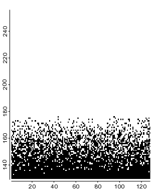
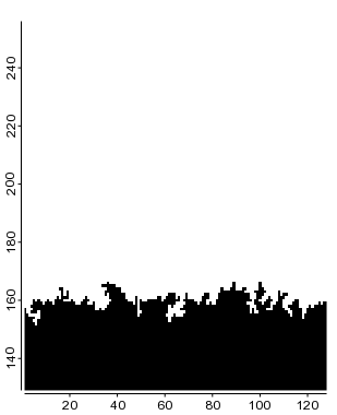
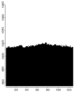
Figure 2: Snapshots from the simulations showing clear differences between two distinct regions. The two upper images are from the same system, a system with a high Young’s modulus, while the two lower images are from a simulation with a low Young’s modulus. The leftmost images are direct printouts, whilst the rightmost images have been filtered to find the largest connected damage cluster, yielding the crack front. These images are the basis for a solid-on-solid analysis, to remove the overhangs. Note the difference in needed filtering between the two regions.

The choice of gradient in the system has an impact. In the results we present here, we have chosen a gradient that clearly demonstrates the different behaviors. A more complete study of the gradient effects will be presented elsewhere. For now, suffice to say that too steep a gradient will constrain the crack front to a smaller width, to the extreme limit where the crack front spans only one or two pixels. Setting a too low gradient will have the effect of increasing the width of the front to the point of the width of the crack front surpassing the length of the system. Zero gradient amounts to pulling the system apart, generating two parallel surfaces, but no crack front.

To analyze the front, we do a solid-on-solid (SOS) thus removing the overhangs. Then we do an averaged wavelet coefficient (AWC) analysis [15, 16], to determine the roughness exponent of the front. The AWC method consists of first doing a wavelet transform of the front $h(x)$, and then, for each length scale $a$, averaging the resulting wavelet coefficients $w(a,b)$ over position $b$ along the front. For self-affine signals, the averaged coefficients $W(a)=\langle|w(a,b)|\rangle_{b}$, should scale as

$$W(a)\sim a^{\zeta+1/2}.$$ (7)

The result of this analysis is shown in Figure 3, giving a roughness exponent of

$$\zeta_{1}=0.45$$

for the stiff system in Figure 3(a), and

$$\zeta_{2}=0.3$$

for the soft system in Figure 3(b). We note that these values are lower than the values reported in the experiments [9] and in the numerical studies, $\zeta_{\textrm{c}}=0.6$ seen in the coalescence model [8] and $\zeta_{\textrm{l}}=0.39$ seen in the fluctuating line model [7]. We also show the data for a smaller system size in the same figure. We see that those data would have given lower values for the roughness exponents. Hence, we believe that the largest system sizes we have presented here are still too small for the effective roughness exponents to have attained their asymptotic values. We are currently testing several methods for running our code on massive parallel computer systems to increase the range of available system sizes.

If we do a small size analysis based on equations (2) and (3), and equation (6), using values from Schmittbuhl and Måløy [6] where they found a response of plexiglass of $F\sim 1$N at a displacement of $\delta=0.1$mm and a Young’s modulus of $E\approx 3.3$GPa, and assuming that the area covered by a single fiber is smaller than $\delta$, we find that the system sizes we have covered so far have room for forces acting at distances of the order of $0.1\sim 1$mm. A system of $L=1024$ would probably reach on the order of 10mm, which would cover the range of the data used for the analysis of the experiment in both [6] and [9]. Based on the results of Santucci et al. [9], we believe that at larger system sizes we will find a crossover between the different scaling behaviors in the same simulation.

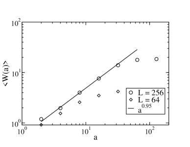
(a) Stiff system

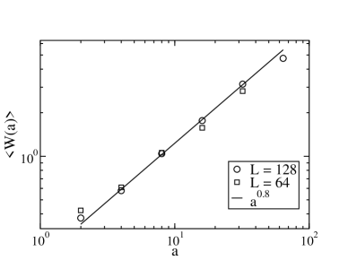
(b) Soft system

Figure 3: Log-log plot of the average wavelet coefficients of a front extracted from the stiff region and from the soft region. Decent power laws are observed, indicating self-affine behavior of two different exponents. Two system sizes are plotted, indicating that the scaling exponents have not yet reached their asymptotic values, so that our results are underestimations.

6 Conclusions

We have shown that our model contains a transition from one regime characterized by a scaling exponent of $\zeta_{1}=0.45$, to another regime characterized by a lower exponent of $\zeta_{2}=0.3$. This transition is achieved through the variation of a single parameter, the Young’s modulus. We believe that these roughness exponents are slight underestimations of the exponents found in the coalescence model and fluctuating line model, respectively, making our model the first to capture these two fracture mechanisms simultaneously — and that the idea that the two roughness regimes seen in the experiments [9] indeed is correct.

References

References

- [1] Mandelbrot B B, Passoja D E and Paullay A J 1984 Nature 308 721
- [2] Bouchaud E, Lapasset G and Planès J 1990 Europhys. Lett. 13 73
- [3] Bonamy D and Bouchaud E 2011 Phys. Rep. 498 1
- [4] Bouchaud J P, Bouchaud E, Lapasset G and Planès J 1993 Phys. Rev. Lett. 71 2240
- [5] Schmittbuhl J, Roux S, Vilotte J-P and Måløy K J 1995 Phys. Rev. Lett. 74 1787
- [6] Schmittbuhl J and Måløy K J 1997 Phys. Rev. Lett. 78 3888
- [7] Rosso A and Krauth W 2002 Phys. Rev. E 65 R025101
- [8] Schmittbuhl J, Hansen A and Batrouni G G 2003 Phys. Rev. Lett. 90 045505
- [9] Santucci S, Grob M, Toussaint R, Schmittbuhl J, Hansen A, and Måløy K J 2010 Europhys. Lett. 92 44001
- [10] Batrouni G G, Hansen A, and Schmittbuhl J 2002 Phys. Rev. E 65 036126
- [11] Pradhan S, Hansen A and Chakrabarti B K 2010 Rev. Mod. Phys. 82 499
- [12] Johnson K L 1985 Contact Mechanics (Cambridge: Cambridge University Press)
- [13] Love A E H 1929 Phil. Trans. R. Soc. A 228 377-420
- [14] Batrouni G G and Hansen A 1988 J. Stat. Phys. 52 747
- [15] Mehrabi A R, Rassamdana H, and Sahimi M 1997 Phys. Rev. E 56 712
- [16] Simonsen I, Hansen A, and Nes O M 1998 Phys. Rev. E 58 2779