Unified decoupling scheme for exchange and anisotropy contributions and temperature-dependent spectral properties of anisotropic spin systems

Abstract

We compute the temperature-dependent spin-wave spectrum and the magnetization for a spin system using the unified decoupling procedure for the high-order Green’s functions for the exchange coupling and anisotropy, both in the classical and quantum case. Our approach allows us to establish a clear crossover between quantum-mechanical and classical methods by developing the classical analog of the quantum Green’s function technique. The results are compared with the classical spectral density method and numerical modeling based on the stochastic Landau-Lifshitz equation and the Monte Carlo technique. As far as the critical temperature is concerned, there is a full agreement between the classical Green’s functions technique and the classical spectral density method. However, the former method turns out to be more straightforward and more convenient than the latter because it avoids any a priori assumptions about the system’s spectral density. The temperature-dependent exchange stiffness as a function of magnetization is investigated within different approaches.

I Introduction

Spin systems offer a rich area for fundamental research, always providing us with new open and challenging issues. In the context of modern applications, magnetic systems at the nanoscale have opened a huge laboratory for testing and applying the available methods with the challenge to adapt them to the constraints of the new area of magnetic nanotechnology. Indeed, the rapid development of computers has opened a new trend for the magnetic materials design. Today the large scale materials modeling is often used as an efficient way to find optimal material performance in technological applications such as magnetic recording. The micromagnetic simulations represent now a powerful tool, especially after the development of publicly available software codes. To provide reliable predictions, the modeling methods should be improved with the incorporation of detailed information from microscopic materials parameters into the macroscopic parameters such as magnetization, anisotropy or exchange stiffness. An additional problem arises when the full-fledged well-known approaches have to be extended to finite-size systems with acute boundary problems.

Furthermore, multiple recent applications require temperature-dependent macroscopic properties. These important applications include heat-assisted magnetic recording citenamefontR. E. Rottmayer et al. (2006), laser-induced magnetization dynamics citenamefontU. Atxitia, O. Chubykalo-Fesenko, N. Kazantseva, D. Hinzke, U. Nowak, and R. W. Chantrell (2007), thermally-assisted magnetic random memories citenamefontI. L. Prejbeanu, M. Kerekes, R. C. Sousa, O. Redon, B. Dieny, and J.P.Nozeires (2007) and thermally-assisted domain wall motion citenamefontD. Hinzke and U. Nowak (2011). In this context the multi-scale scheme where the temperature-dependent macroscopic parameters are previously calculated numerically or analytically with the aim to use them in larger scale modeling has been proposed citenamefontN. Kazantseva, D. Hinzke, U. Nowak, R. W. Chantrell, U. Atxitia, and O. Chubykalo-Fesenko (2008); citenamefontU. Atxitia, D. Hinzke, O. Chubykalo-Fesenko, U. Nowak, H. Kachkachi, O. N. Mryasov, R. F. Evans, R. W. Chantrell (2010). The variety of methods, classical and quantum, analytical and numerical, were developed in the past and can be adjusted today for applications within this multi-scale modeling framework. It is then necessary to take stock of the various methods, compare them and establish their respective limits of applicability. This is a tremendous task that has to be tackled before one can apply these methods to design new magnetic materials.

Accordingly, the present work is about a few standard methods used for investigating the spectrum of spin waves (SW) in magnetic systems at finite temperature and for arbitrary spin. These are the quantum Green’s function (QGF) technique and its classical limit (CGF), the classical spectral density (CSD) method, and the purely numerical methods, i) one that consists in solving the stochastic Landau-Lifshitz equation (LLE) citenamefontW. F. Brown (1963); citenamefontA. Lyberatos and R.W. Chantrell (1993) and ii) the Metropolis Monte Carlo (MC) method citenamefontBinder and Heermann (1992). Although these methods exist in the literature in different and multiple formulations, no systematic comparison with the aim to establish their agreement and crossover has been made. One of our objectives here is to compare these methods and establish the best framework for the calculation of the temperature-dependent SW spectrum and physical observables such as the magnetization and susceptibility. For each method we discuss the most reliable implementation which gives the best agreement with numerical techniques and provide a clear crossover between the classical and the quantum case. In this task we have realized that no unified decoupling scheme used to take into account both the exchange and anisotropy contributions in the classical case has been given in the literature so far. However, this is exactly what is required for the purpose of the hierarchical multi-scale modeling, where classical Heisenberg-like Hamiltonian is parameterized via ab initio calculations and is used to evaluate temperature-dependent macroscopic properties citenamefontN. Kazantseva, D. Hinzke, U. Nowak, R. W. Chantrell, U. Atxitia, and O. Chubykalo-Fesenko (2008); citenamefontU. Atxitia, D. Hinzke, O. Chubykalo-Fesenko, U. Nowak, H. Kachkachi, O. N. Mryasov, R. F. Evans, R. W. Chantrell (2010). On the other hand, in the future the use of classical systems may be avoided if direct reliable calculations of macroscopic properties at the nanoscale based on quantum spin systems are available. This is why it is important to establish clear connection between quantum and classical approaches.

It is well known that the Green’s function and spectral density methods involve a decoupling of high-order spin correlations into two-point correlations. Here we revisit this issue and demonstrate a clear connection between, on one hand, the classical and quantum approaches, and on the other, the CGF technique and the CSD method. In the quantum case, the spin operators satisfy the $SU(2)$ Lie algebra and this implies that two spin operators commute when they refer to distinct lattice sites. In particular, the longitudinal and transverse spin fluctuations are uncorrelated when they refer to two distinct lattice sites and they are strongly correlated otherwise. However, a decoupling that may be successful in dealing with the exchange coupling contribution, at least at low temperature, may turn out to be a bad approximation for the local (with identical lattice sites) contributions of (on-site) anisotropy. This is why mean-field theory (MFT), random-phase approximation (RPA) and the Bogoliubov-Tyablikov approximation (BTA), which assume that the longitudinal and transverse fluctuations are uncorrelated, provide a reasonably good approximation for exchange whereas they provide rather poor results in the presence of anisotropy.

Here we pay a special attention to this issue and considerably clarify the situation regarding the decoupling scheme that is used for exchange and anisotropy contributions. More precisely, we provide a unified decoupling scheme for both exchange and anisotropy contributions, for classical as well as quantum spins. Then, using this decoupling we obtain workable (semi-)analytical expressions for the SW dispersion, the magnetization and the critical temperature, which are supported by the good agreement with the numerical results of the LLE method and Monte Carlo (MC) simulations.

In section II we define the generic system we study using the Dirac-Heisenberg Hamiltonian. In section III, we discuss the various decoupling schemes used in QGF technique and show how they are related, and compute the SW dispersion and the magnetization. For the latter we also provide the analytical asymptotes at low temperature and near the critical point. Next, we work out the classical limit of this approach and obtain the corresponding dispersion and magnetization. For the latter, we pinpoint an interesting connection between the Callen’s (quantum) expression for the magnetization and the MFT-like expression in terms of the Brillouin function in the quantum case. Apart from its elegance, this formulation makes it straightforward to derive the classical limit in terms of the Langevin function. We then turn to the CSD method and clarify the relevance of the decoupling scheme when it comes to treat the exchange coupling and anisotropy. We end this section with a brief account of the LLE and MC methods and a few expressions and numerical estimates of the critical temperature. Section IV.1 presents the results for the SW spectrum, the magnetization as a function temperature and field, and spin stiffness. The paper ends with a conclusion and outlook. In Appendices A we present the main steps of the QGF for finite temperature, arbitrary spin, and oblique magnetic field. In appendix B, we give a detailed demonstration of some expressions used within the CSD approach. In appendix C we give a few expressions and numerical estimates for the critical temperature.

II Model: Hamiltonian and system studied

We study a spin system of $\mathcal{N}$ atomic spins $\mathbf{S}_{i}=S\mathbf{s}_{i}$, with $\left|\mathbf{s}_{i}\right|=1$, interacting via a nearest-neighbor exchange coupling $J_{ij}$. In addition, each spin evolves in a (local) potential energy that comprises an on-site anisotropy and a Zeeman contribution. The anisotropy is taken uniaxial with a common easy axis pointing in the $z$ direction; the magnetic field is applied in an arbitrary direction $\mathbf{e}_{h}$ so that $\mathbf{H}=H\mathbf{e}_{h}$. The Hamiltonian of the system then reads

$$\mathcal{H}=-\frac{1}{2}\sum_{\left\langle i,j\right\rangle}J_{ij}\,\mathbf{S}_{i}\cdot\mathbf{S}_{j}-K\sum_{i=1}^{\mathcal{N}}\left(S_{i}^{z}\right)^{2}-\left(g\mu_{B}H\right){\displaystyle{\displaystyle\sum_{i=1}^{\mathcal{N}}}}\mathbf{S}_{i}\cdot\mathbf{e}_{h}.$$ (1)

We consider only box-shaped systems of size $N_{x}\times N_{y}\times N_{z}=\mathcal{N}$ with, e.g. a simple cubic (sc) or a body-centered-cubic (bcc) lattice structure.

III Methods

We would like to investigate the spectral properties of such systems using and comparing two groups of methods: i) the (semi-)analytical methods, namely the classical spectral density method and the classical or quantum methods of Green’s functions (GF) at finite temperature, ii) the numerical methods that consist either in solving the stochastic Landau-Lifshitz-Gilbert equation (LLE) in the Langevin approach or Monte Carlo (MC) simulations.

III.1 Quantum Green’s function approach

The Green’s function approach has been used thoroughly in almost all areas of physics. For spin systems, this approach allows us to obtain and investigate all kinds of observables. As compared to spin-wave theory (SWT), it makes it possible to obtain in a more systematic way the excitation spectrum at finite temperature for arbitrary atomic (nominal) spin.

For our present purposes, we re-derive the basic equations involved in this approach and apply them to the Hamiltonian (1). In the latter the magnetic field is applied in an arbitrary direction with respect to the (common) anisotropy easy axis and as such, a slight reformulation of the basic equations is needed with respect to the equilibrium configuration. In particular, Callen’s formula (citenamefontA. I. Akhiezer, V. G. Bar’yakhtar, and S. V. Peletminskii, 1968) for the magnetization in the case of arbitrary spin has to be re-derived in this context. The details of these calculations are given in Appendix A.

We introduce the retarded many-body Green’s functions

$$\mathcal{G}^{\mu\nu}(i-j,t) =\mathcal{G}^{\mu\nu}(\mathbf{r}_{i}-\mathbf{r}_{j},t)\equiv\left\langle\left\langle\sigma_{i}^{\mu}(t);\sigma_{j}^{\nu}(0)\right\rangle\right\rangle_{r}=-i\theta(t)\left\langle\left[\sigma_{i}^{\mu}(t),\,\sigma_{j}^{\nu}(0)\right]\right\rangle.$$ (2)

where $\bm{\sigma}_{i}$ are the new spin variables obtained after rotation of the original variables $\mathbf{S}_{i}$ to the system of coordinates where the $z$-axis coincides with the direction of the net magnetization [see Appendix A]; $\left\langle\ldots\right\rangle$ denotes the usual thermal average. Then, one establishes the equations of motion of the GFs $\mathcal{G}_{ij}^{+-}$, $\mathcal{G}_{ij}^{--}$, $\mathcal{G}_{ij}^{3-}$ whose solution renders the SW dispersion.

The equation of motion for a GF of a given order in spin operators generates GFs of higher orders and this leads to an infinite hierarchy of GFs satisfying an open system of coupled equations. In order to close this system of equations and solve it (in Fourier space), one is led to apply a certain scheme for breaking high-order GFs into lower-order ones, thus adopting a certain approximation of the magnon-magnon interactions. Finding an adequate scheme for doing so has triggered many investigations each dealing with a specific situation with a particular Hamiltonian. Unfortunately, there is no general or systematic procedure. In fact, the variety of decoupling schemes only reflects the complexity of dealing with magnon-magnon interactions and thereby the nonlinear SW effects. In the following section, we present a discussion of the main decoupling schemes known in the literature and also propose some improvements that allow for a certain unification thereof.

III.1.1 Decoupling schemes

When applying mean-field theory (MFT), random-phase approximation (RPA), or the Bogoliubov-Tyablikov approximation (BTA), it is implicitly assumed that the longitudinal and transverse fluctuations are uncorrelated and this is a valid approximation only when they refer to distinct sites. Indeed, the idea behind this approximation consists in writing

$$\left\langle\left[AB,\,C\right]\right\rangle\simeq\left\langle A\right\rangle\times\left\langle\left[B,\,C\right]\right\rangle.$$ (3)

For spin systems, the factor $\left\langle A\right\rangle$ is usually the thermal average of $\sigma^{3}$ and thereby is related to the temperature-dependent magnetization. Hence, in practice one rearranges the various terms so that $\sigma^{3}$ appears on the left and then use the approximation (3). However, in the (local) anisotropy contributions the product factors are at the same site and thus the longitudinal and transverse fluctuations are correlated, which turns this kind of decoupling schemes into relatively bad approximations.

In Ref. (citenamefontJ. F. Devlin, 1971) it was argued that one may avoid this approximation inherent to a decoupling scheme by establishing $2S$ equations of motion for the anisotropy functions. The problem with this approach, however, is that in practice one has to specify the spin $S$ thus limiting the calculations to a particular material. In addition, it is not obvious how to obtain the classical limit from the final results.

For the exchange coupling, RPA is commonly used with reasonable satisfaction since the corresponding results for the SW dispersion and thereby the magnetization compare fairly well with other techniques such as Monte Carlo (MC) [see Ref. (citenamefontP. Frobrich, P.J. Kuntz, 2006) for a recent review], as long as the magnetization curve at low temperature is concerned. However, for a more precise estimation of the critical temperature $T_{C}$, Callen’s decoupling scheme turns out to be much more efficient, though it leads to a self-consistent equation for $T_{C}$ which is more difficult to tackle analytically. Indeed, it was shown by Tahir-Kheli and Callen citenamefontR. A. Tahir-Kheli and H. B. Callen (1964); citenamefontR. A. Tahir-Kheli (1976); citenamefontH. B. Callen (1963) that the more sophisticated decoupling scheme

$$\left\langle\left\langle\sigma_{i}^{3}(\tau)\sigma_{l}^{+}(\tau);\sigma_{j}^{-}(0)\right\rangle\right\rangle \underset{i\neq j}{\simeq}\left\langle\sigma_{i}^{3}\right\rangle\left\langle\left\langle\sigma_{l}^{+}(\tau);\sigma_{j}^{-}\left(0\right)\right\rangle\right\rangle-\left\langle\sigma_{i}^{3}\right\rangle\frac{\left\langle\sigma_{i}^{-}\sigma_{l}^{+}\right\rangle}{2S^{2}}\left\langle\left\langle\sigma_{i}^{+}(\tau);\sigma_{j}^{-}\left(0\right)\right\rangle\right\rangle$$ (4)

takes, to some extent, account of magnon-magnon interactions and renders a nonlinear equation for the magnon dispersion $\omega(\mathbf{k})$, see below.

For on-site magneto-crystalline anisotropy the simplistic RPA decoupling leads to poor and even wrong results. In the presence of anisotropy with typical ratios $K/J$, the Anderson-Callen decoupling scheme, originally proposed by Anderson and Callen (citenamefontH. B. Callen, 1963; citenamefontF. B. Anderson and H. B. Callen, 1964) and later generalized by Schwieger et al. (citenamefontS. Schwieger, J. Kienert, and W. Nolting, 2005) to a rotated reference frame, turns out to be rather efficient in producing reasonable results. This is typically of the form

$$K\left\langle\left\langle\left(\sigma_{i}^{3}\sigma_{i}^{-}+\sigma_{i}^{-}\sigma_{i}^{3}\right)\left(t\right);\,\sigma_{j}^{-}\left(0\right)\right\rangle\right\rangle \approx 2\mathcal{K}_{\sigma}\left\langle\sigma_{i}^{3}\right\rangle\times\left\langle\left\langle\sigma_{i}^{-}\left(t\right);\,\sigma_{j}^{-}\left(0\right)\right\rangle\right\rangle,$$ (5)

with the effective anisotropy factor

$$\mathcal{K}_{\sigma}=K\left[1-\frac{1}{4S^{2}}\left(\left\langle\sigma_{i}^{+}\sigma_{i}^{-}\right\rangle+\left\langle\sigma_{i}^{-}\sigma_{i}^{+}\right\rangle\right)\right].$$ (6)

The identity

$$\left\langle\sigma_{i}^{+}\sigma_{i}^{-}\right\rangle+\left\langle\sigma_{i}^{-}\sigma_{i}^{+}\right\rangle=2S(S+1)-2\left\langle\sigma_{i}^{3}\sigma_{i}^{3}\right\rangle,$$

is derived from the quantum-mechanical identities

$$\sigma^{-}\sigma{}^{+} =S(S+1)-\left(\sigma^{3}\right)^{2}-\sigma^{3},$$

$$\sigma^{3} =\frac{1}{2}\left(\sigma^{+}\sigma^{-}-\sigma^{-}\sigma^{+}\right).$$ (7)

It is well known that the decoupling (5) is valid for all spin values $S$ and renders good results when compared with the exact treatment of anisotropy and with quantum MC when $K/J$ is small (citenamefontP. Frobrich, P.J. Kuntz, 2006) .

Similar to the decoupling in Eq. (5), the following decoupling for anisotropy has been suggested citenamefontF. B. Anderson and H. B. Callen (1964)

$$\left\langle\left\langle\sigma_{i}^{3}(\tau)\sigma_{i}^{+}(\tau)+\sigma_{i}^{3}(\tau)\sigma_{i}^{+}(\tau);\sigma_{j}^{-}\left(0\right)\right\rangle\right\rangle =\left\langle\sigma_{i}^{3}\right\rangle\left[2-\frac{\left\langle\sigma_{i}^{-}\sigma_{i}^{+}\right\rangle+\left\langle\sigma_{i}^{+}\sigma_{i}^{-}\right\rangle}{2S^{2}}\right]\left\langle\left\langle\sigma_{i}^{+}(\tau);\sigma_{j}^{-}\left(0\right)\right\rangle\right\rangle$$

Then, splitting the right-hand side as follows

$$\left\langle\sigma_{i}^{3}\right\rangle\left[2-\frac{\left\langle\sigma_{i}^{-}\sigma_{i}^{+}\right\rangle+\left\langle\sigma_{i}^{+}\sigma_{i}^{-}\right\rangle}{2S^{2}}\right]\left\langle\left\langle\sigma_{i}^{+}(\tau);\sigma_{j}^{-}\left(0\right)\right\rangle\right\rangle =\left\langle\sigma_{i}^{3}\right\rangle\left(1-\frac{\left\langle\sigma_{i}^{+}\sigma_{i}^{-}\right\rangle}{2S^{2}}\right)\left\langle\left\langle\sigma_{i}^{+}(\tau);\sigma_{j}^{-}\left(0\right)\right\rangle\right\rangle$$

$$+\left\langle\sigma_{i}^{3}\right\rangle\left(1-\frac{\left\langle\sigma_{i}^{-}\sigma_{i}^{+}\right\rangle}{2S^{2}}\right)\left\langle\left\langle\sigma_{i}^{+}(\tau);\sigma_{j}^{-}\left(0\right)\right\rangle\right\rangle$$

we may propose the following decoupling

$$\left\langle\left\langle\sigma_{i}^{3}(\tau)\sigma_{i}^{+}(\tau);\sigma_{j}^{-}\left(0\right)\right\rangle\right\rangle =\left\langle\sigma_{i}^{3}\right\rangle\left[1-\frac{\left\langle\sigma_{i}^{-}\sigma_{i}^{+}\right\rangle}{2S^{2}}\right]\times\left\langle\left\langle\sigma_{i}^{+}(\tau);\sigma_{j}^{-}\left(0\right)\right\rangle\right\rangle.$$ (8)

Comparing this decoupling for the anisotropy contribution with Eq. (4) for the exchange contribution, we see that the former follows from the latter upon setting in the latter $l=i$, i.e., restricting the product of spin operators to the same lattice site. In fact, this is a consequence of the way $\sigma_{i}^{3}$ is written in powers of $\sigma_{i}^{3}$ and the products $\sigma_{i}^{\pm}\sigma_{j}^{\mp}$. More precisely, if we start from the quantum-mechanical identities (7) and then multiply them by $\alpha$ and $1-\alpha$ respectively and add the resulting equations we obtain

$$\sigma^{3} =\alpha S(S+1)-\alpha\left(\sigma^{3}\right)^{2}+\left(\frac{1-\alpha}{2}\right)\sigma^{+}\sigma^{-}-\left(\frac{1+\alpha}{2}\right)\sigma^{-}\sigma{}^{+},$$ (9)

where $\alpha$ is then determined so as to comply with the limits at zero temperature and near the critical point citenamefontH. B. Callen (1963). This leads to $\alpha=\left\langle\sigma^{3}\right\rangle/2S^{2}$.

Next, we insert the expression (9) for $\sigma^{3}$ in products of spin operators such as those appearing on the left-hand side of Eqs. (4, 8) and use Wick’s or RPA-like decoupling to obtain the decoupling (4) for exchange and (8) for anisotropy contributions, respectively. In fact, there exist several other decoupling schemes in the literature with expressions for $\alpha$ that are polynomials of different degrees in $m=\left\langle\sigma^{3}\right\rangle/S$. Namely, $\alpha=0$ corresponds to RPA (or BTA), $\alpha\propto m$ to Callen’s decoupling, $\alpha\propto m^{3}$ to the decoupling proposed by Copeland and Gersch (CG) citenamefontJ. A. Copeland and H. A. Gersch (1966), and

$$\alpha\left(m\right)=\frac{1}{2}\frac{S-1}{S\left(S+1\right)}m+\frac{1}{S\left(S+1\right)}m^{3}$$ (10)

to the decoupling proposed later by Swendsen citenamefontR. H. Swendsen (1972).

As already discussed, these polynomials with increasing degrees are approximations to the more rigorous calculation of spin correlations that consists in computing contributions of high-order of Feynman’s spin diagrams as is done in Refs. citenamefontYu. A. Izyumov and Yu. N. Skryabin, 1988; citenamefontD. A. Garanin and V. S. Lutovinov, 1984. As it will be seen later in section IV.1, the corresponding decoupling yields fairly precise results for the magnetization and critical temperature.

III.1.2 Spin-wave dispersion

Applying for instance the RPA decoupling to a homogeneous ferromagnet, i.e. with $\left\langle\sigma_{i}^{3}\right\rangle=\left\langle\sigma^{3}\right\rangle$, (see details in Appendix A) one derives the magnon energy with respect to the equilibrium state

$$E^{2}(\mathbf{k}) = \left(\hbar\omega(\mathbf{k})\right)^{2}=\mathcal{A}_{\mathbf{k}}^{2}-\mathcal{B}_{\mathbf{k}}^{2}$$

$$= \left[\left(g\mu_{B}\right)\left(H^{x}\sin\vartheta+H^{z}\cos\vartheta\right)+\mathcal{K}_{\sigma}\left\langle\sigma^{3}\right\rangle\left(2\cos^{2}\vartheta-\sin^{2}\vartheta\right)+J_{0}\left\langle\sigma^{3}\right\rangle\left(1-\gamma_{\mathbf{k}}\right)\right]^{2}$$

$$-\left(\mathcal{K}_{\sigma}\right)^{2}\left\langle\sigma^{3}\right\rangle^{2}\sin^{4}\vartheta.$$

where [see Appendix A for notation]

$$\begin{array}[]{lll}\mathcal{A}_{\mathbf{k}}&\equiv&L^{3}+\mathcal{K}_{\sigma}\left\langle\sigma^{3}\right\rangle\left(2\cos^{2}\vartheta-\sin^{2}\vartheta\right)+J_{0}\left\langle\sigma^{3}\right\rangle\left(1-\gamma_{\mathbf{k}}\right),\\ \mathcal{B}_{\mathbf{k}}&\equiv&\mathcal{K}_{\sigma}\left\langle\sigma^{3}\right\rangle\sin^{2}\vartheta\end{array}$$ (12)

$J_{0}=J\left(0\right)$ being defined in Eq. (82).

This dispersion relation is effectively obtained within the linear spin-wave theory, because the high-order GFs stemming from exchange contributions have been decoupled using the RPA which does not take account of spin correlations or magnon-magnon interactions. Indeed, following the standard procedure described in the appendix of Ref. (citenamefontU. Atxitia, D. Hinzke, O. Chubykalo-Fesenko, U. Nowak, H. Kachkachi, O. N. Mryasov, R. F. Evans, R. W. Chantrell, 2010) (and references therein) one arrives at the equation for the dispersion (in the case $\vartheta=0$, i.e., of longitudinal field and $\left\langle\sigma_{i}^{3}\right\rangle=\left\langle S_{i}^{z}\right\rangle$)

$$\hbar\omega\left(\mathbf{k}\right)\equiv\hbar\omega_{\mathbf{k}} =\left(g\mu_{B}\right)H+2\mathcal{K}_{S}\left\langle S^{z}\right\rangle+\left\langle S^{z}\right\rangle\left[J(0)-J(\mathbf{k})\right]+\frac{\left\langle S^{z}\right\rangle}{\mathcal{N}S}\alpha\sum_{\mathbf{p}}\left[J(\mathbf{p})-J(\mathbf{p}-\mathbf{k})\right]\left\langle n_{\mathbf{p}}\right\rangle,$$ (13)

where $\mathcal{K}_{S}$ reads,

$$\mathcal{K}_{S}=\mathcal{K}_{\sigma}\left(\vartheta=0\right)=K\left[1-\frac{1}{2S^{2}}\left(S(S+1)-\left\langle S^{z}S^{z}\right\rangle\right)\right]$$ (14)

and $\alpha=m$ for Callen’s decoupling. $\left\langle n_{\mathbf{p}}\right\rangle$ is the thermal occupation number given by the magnon Bose-Einstein distribution

$$\left\langle n_{\mathbf{p}}\right\rangle=\frac{1}{e^{\beta\hbar\omega_{\mathbf{p}}}-1}$$ (15)

where $\beta=1/k_{\mathrm{B}}T$.

Then, using translation invariance we see that

$$\frac{J(\mathbf{p})-J(\mathbf{p}-\mathbf{k})}{J(0)-J(\mathbf{k})}=\frac{\gamma_{\mathbf{p}}-\gamma_{\mathbf{p}\mathbf{-k}}}{1-\gamma_{\mathbf{k}}}=\gamma_{\mathbf{p}}$$

and thereby

$$\hbar\omega_{\mathbf{k}} =\left(g\mu_{B}\right)H+2\mathcal{K}_{S}\left\langle S^{z}\right\rangle+J_{0}\left\langle S^{z}\right\rangle Q\left(\alpha,\beta\right)\left(1-\gamma_{\mathbf{k}}\right).$$ (16)

Here we have introduced the exchange “stiffness coefficient”

$$Q(\alpha,\beta) =1+\frac{\alpha}{\mathcal{N}S}\sum_{\mathbf{p}}\frac{\gamma_{\mathbf{p}}}{e^{\beta\hbar\omega_{\mathbf{p}}}-1}=1+\frac{\alpha}{\mathcal{N}S}\sum_{\mathbf{p}}\gamma_{\mathbf{p}}\left\langle n_{\mathbf{p}}\right\rangle$$ (17)

where $\alpha$ is, as defined earlier, depends on the decoupling scheme.

III.1.3 Magnetization

Now, we turn to compute the magnetization for an arbitrary spin $S$. In Callen’s method [see Ref. (citenamefontA. I. Akhiezer, V. G. Bar’yakhtar, and S. V. Peletminskii, 1968) and references therein] one considers the GF

$$\Xi^{\mu\nu}(i-j,t;\xi)=-i\theta(t)\times\left\langle\left[\sigma_{i}^{\mu}(t),\exp(\xi\sigma_{j}^{z}(0))\;\sigma_{j}^{\nu}(0)\right]\right\rangle.$$ (18)

Then, replacing the GFs in the system (88) by their analogs from Eq. (18) we obtain the new system of EM

$$\left\{\begin{array}[]{ccc}\left(\omega-\mathcal{A}_{\mathbf{k}}\right)\Xi_{\mathbf{k}}^{+-}+\mathcal{B}_{\mathbf{k}}\Xi_{\mathbf{k}}^{--}&=&\left\langle\left[\sigma_{i}^{+}(0),\exp(\xi\sigma_{i}^{z}(0))\;\sigma_{i}^{-}(0)\right]\right\rangle\equiv\Sigma^{+-}\\ \\ -\mathcal{B}_{\mathbf{k}}\Xi_{\mathbf{k}}^{+-}+\left(\omega+\mathcal{A}_{\mathbf{k}}\right)\Xi_{\mathbf{k}}^{--}&=&0.\end{array}\right.$$ (19)

Following again Callen’s procedure we obtain for the first moment $\left\langle\sigma^{3}\right\rangle$

$$\left\langle\sigma^{3}\right\rangle=\frac{(S-\Omega)(1+\Omega)^{2S+1}+(S+1+\Omega)\Omega^{2S+1}}{(1+\Omega)^{2S+1}-\Omega^{2S+1}}.$$ (20)

where $\Omega$ is the following function of the $1^{\mathrm{st}}$ and $2^{\mathrm{nd}}$ moments $\left\langle\sigma^{3}\right\rangle,\left\langle\sigma^{3}\sigma^{3}\right\rangle\equiv\mathcal{C}^{33}$,

$$\Omega\left(\left\langle\sigma^{3}\right\rangle,\mathcal{C}^{33}\right)=\frac{1}{2}\frac{1}{N_{c}}\sum_{\mathbf{k}}\left[\frac{\mathcal{A}_{\mathbf{k}}}{\omega_{\mathbf{k}}}\coth\left(\frac{\beta\hbar\omega_{\mathbf{k}}}{2}\right)-1\right].$$ (21)

$N_{c}$ is the number of unit cells in the Bravais lattice of the ferromagnet and is also the number of allowed wave-vectors in the Brillouin zone.

Eq. (20), together with (16) and (21), constitutes a transcendental equation whose solution involves several sums (integrals) in Fourier space. In general, it is a heavy task to solve Eq. (20) especially for lattices with several sub-lattices. Nonetheless, it was shown in Ref. (citenamefontH. B. Callen and S. Strikman, 1965) that the magnetization $\bar{\sigma}\equiv\left\langle\sigma^{3}\right\rangle$ in Eq. (20) can be recast into the following more compact form

$$\bar{\sigma}=SB_{S}\left[SX\right]$$ (22)

where $X$ is defined by

$$\Omega=\frac{1}{e^{X}-1}$$ (23)

and $B_{S}(x)$ is the Brillouin function (for the quantum spin $S$)

$$B_{S}(x)=\frac{2S+1}{2S}\coth\left[\left(\frac{2S+1}{2S}\right)x\right]-\frac{1}{2S}\coth\left(\frac{x}{2S}\right).$$ (24)

More generally, it was shown (citenamefontE. R. Callen and H. B. Callen, 1965; citenamefontH. B. Callen and S. Strikman, 1965) that the higher moments $\left\langle\bar{\sigma}^{n}\right\rangle$ can all be expressed in terms of the reduced magnetization $m=\bar{\sigma}/S$ whereby the temperature $T$ and field $H$ enter via $m=m\left(T,H\right)$. It was argued that this model-independent MFT-like result stems from the exponential form of the probability density, i.e., $\rho=e^{XS^{z}}/\mathrm{Tr}\,e^{XS^{z}}$. Indeed, Eq. (23) expresses the fact that in MFT all the excitations are degenerate and that one may define the energy $\varepsilon=X/k_{\mathrm{B}}T$ as the effective energy of the molecular-field-like excitations with the same occupation number as the true excitations. On the other hand, we note that Eq. (22) is also a transcendental equation for $\bar{\sigma}$, similar to Eq. (20), though much more compact and it readily yields the classical limit, as will be seen below. In addition, this establishes the connection to the standard result of MFT.

In order to solve either equation, i.e. (20) or (22), and obtain the magnetization $m\left(T,H\right)$ one has to supplement the latter by a second equation for the correlation function $\mathcal{C}^{33}=\left\langle\sigma^{3}\sigma^{3}\right\rangle$; this is obtained by the Callen’s procedure (for $\xi=0$, see Eq. (18)) which leads to

$$\left\langle\sigma_{i}^{-}\sigma_{i}^{+}\right\rangle = 2\bar{\sigma}\times\Omega\left(\bar{\sigma},\mathcal{C}^{33}\right).$$ (25)

together with $1^{\mathrm{st}}$ the identity in Eq. (7).

The latter also yields

$$\left\langle\sigma^{3}\sigma^{3}\right\rangle = S\left(S+1\right)-\bar{\sigma}-\left\langle\sigma^{-}\sigma^{+}\right\rangle=S\left(S+1\right)-\left(1+2\Omega\right)\bar{\sigma}.$$ (26)

Finally, the magnetization (in the rotated frame) $\bar{\sigma}$ is given by the solution of the following system of two nonlinear (coupled) equations

$$\left\{\begin{array}[]{ccc}\bar{\sigma}&=&SB_{S}\left[S\ln\left(1+\frac{1}{\Omega}\right)\right],\\ \\ \mathcal{C}^{33}&=&S\left(S+1\right)-\left(1+2\Omega\right)\bar{\sigma}.\end{array}\right.$$ (27)

In general, this system can only be solved numerically as it involves transcendental equations with several integrals. However, we can establish a few analytical expressions for the magnetization in the limiting temperature regions $T\rightarrow 0$ and $T\to T_{C}$ and upon restricting ourselves to a longitudinal magnetic field, i.e. applied along the direction $\mathbf{e}_{3}$ ($\psi=0$).

In this case the SW dispersion $\hbar\omega_{\mathbf{k}}$ in Eq. (III.1.2) simplifies into

$$\hbar\omega_{\mathbf{k}}=\mathcal{A}_{\mathbf{k}}=L^{3}+2\mathcal{K}_{\sigma}\bar{\sigma}+J_{0}\bar{\sigma}\left(1-\gamma_{\mathbf{k}}\right)$$

and Eq. (21) becomes

$$\Omega\left(\bar{\sigma},\mathcal{C}^{33}\right)=\frac{1}{N_{c}}\sum_{\mathbf{k}}\frac{1}{2}\left[\coth\left(\frac{\beta\hbar\omega_{\mathbf{k}}}{2}\right)-1\right].$$ (28)

Low temperature asymptote

At low temperature, the spins are strongly correlated and thereby the correlation function $\mathcal{C}^{33}$ tends to $S\left(S+1\right)$. As a consequence, the effective anisotropy obtained from the Anderson-Callen decoupling scheme simply yields $\mathcal{K}_{S}\longrightarrow K$ [see Eq. (14)] so that the system of equations (27) decouples leading to a closed equation for $\bar{\sigma}$ whose solution then is Eq. (20). Expanding the latter in terms of $\Omega$ (which becomes small at low temperature), we find

$$\bar{\sigma}\simeq S-\Omega\left(\bar{\sigma}\right).$$

Moreover, at low temperature only low-energy spin waves are excited and these are the long-wave length modes. Hence, in the limit of small wave vectors, we have the dispersion relation

$$\hbar\omega_{\mathbf{k}}\simeq g\mu_{B}H^{z}+2K\bar{\sigma}+A\bar{\sigma}k^{2},$$ (29)

where $A\equiv J\delta^{2}$, $\delta^{2}\equiv\sum a^{2}J(a)/\sum J(a)$, $a$ is the lattice parameter and $J(a)$ is the exchange coupling over the nearest-neighbor bond.

Next, upon expanding $\Omega$ in terms of temperature $T$ (or rather in $k_{\mathrm{B}}T/J_{0}S$) we obtain

$$\left\langle\sigma^{3}\right\rangle\simeq S-\left(\frac{3\tau}{2\pi S}\right)^{3/2}Z{}_{3/2}\left[\frac{h+\kappa S}{\tau}\right]$$ (30)

where

$$Z_{p}\left(x\right)=\sum_{n=1}^{\infty}n^{-p}e^{-nx},$$

and $Z_{p}\left(0\right)=\zeta\left(p\right)$ is the well known Riemann zeta function. We have also introduced the following dimensionless parameters

$$\tau\equiv\frac{1}{\beta J_{0}}=\frac{k_{\mathrm{B}}T}{J_{0}},\quad h\equiv\frac{\left(g\mu_{B}\right)H}{J_{0}},\quad\kappa\equiv\frac{2K}{J_{0}}.$$

Obviously, in the present limit and in zero applied field, one obtains the well known “$3/2$” Bloch’s power law for the thermal decrease of the magnetization.

Near-critical temperature asymptote ($H=0$)

Just below the Curie temperature, in the absence of magnetic field, the mean number of excited quasi-particles and their density are large, and it is then a reasonable approximation to pass to the continuum limit. In this case, in Eq. (28) we make the transformation

$$\frac{1}{N_{c}}\times\sum_{\mathbf{k}}\left(\cdots\right)_{\mathbf{k}}\longrightarrow\frac{1}{N_{c}}\times\frac{V}{\left(2\pi\right)^{3}}\iiint d^{3}k\,\left(\cdots\right)_{\mathbf{k}}=\frac{V}{N_{c}}\iiint\frac{d^{3}k}{\left(2\pi\right)^{3}}\left(\cdots\right)_{\mathbf{k}}=v_{0}\int\frac{d\mathbf{k}}{\left(2\pi\right)^{3}}\left(\cdots\right)_{\mathbf{k}}$$

where $v_{0}$ is the volume of the unit cell of the direct lattice.

Next, in this limit the system (27) again decouples and leads to the Callen’s expression (20) for the magnetization, similarly to the low-temperature limit. In addition, we may write for $C^{33}$

$$C^{33}\simeq\frac{S\left(S+1\right)}{3}$$ (31)

where the factor $1/3$ stems from the three dimensional rotational symmetry ($SO\left(3\right)$) of spins that starts to recover as the temperature reaches the critical temperature of the ferromagnet.

Consequently, upon inserting in Eq. (13) $\mathcal{C}^{33}=\left\langle S^{z}S^{z}\right\rangle$ given by the result above, dropping the nonlinear SW contributions, and neglecting the second-order terms in $\bar{\sigma}$ we obtain the dispersion

$$\hbar\omega_{\mathbf{k}} =2K\eta\bar{\sigma}+\bar{\sigma}J_{0}\left(1-\gamma_{\mathbf{k}}\right)=J_{0}\bar{\sigma}\lambda^{-1}\left(1-\lambda\gamma_{\mathbf{k}}\right).$$ (32)

with

$$\eta\equiv 1-\frac{S(S+1)}{3S^{2}},\quad\lambda\equiv\frac{1}{1+\eta\kappa}.$$ (33)

In addition, $\bar{\sigma}$ is rather small because the density of SW is large and since $\omega_{\mathbf{k}}$ is proportional to $\bar{\sigma}$, as is seen in Eq. (32), we can expand $\Omega\left(\left\langle\sigma^{3}\right\rangle\right)$ in powers of $\omega_{\mathbf{k}}$ and obtain

$$\Omega\left(\bar{\sigma}\right) =v_{0}\intop\frac{d\mathbf{k}}{\left(2\pi\right)^{3}}\frac{1}{e^{\beta\hbar\omega_{\mathbf{k}}}-1}\simeq v_{0}\intop\frac{d\mathbf{k}}{\left(2\pi\right)^{3}}\left(\frac{1}{\beta\hbar\omega_{\mathbf{k}}}-\frac{1}{2}+\frac{\beta\hbar\omega_{\mathbf{k}}}{12}\right).$$ (34)

Let us now compute these integrals. Using (32), the first contribution reads

$$v_{0}\intop\frac{d\mathbf{k}}{\left(2\pi\right)^{3}}\frac{1}{\beta\hbar\omega_{\mathbf{k}}}=\frac{\lambda P\left(\lambda\right)}{\bar{\sigma}}\tau.$$

where we have introduced the well known lattice Green’s function [see Ref. citenamefontG. S. Joyce, 1972 and references therein]

$$P\left(\lambda\right)\equiv v_{0}\intop\frac{d\mathbf{k}}{\left(2\pi\right)^{3}}\frac{1}{1-\lambda\gamma_{\mathbf{k}}}.$$ (35)

Analytical expressions for this integral for various limiting cases of the parameter $\lambda$ are given in Ref. citenamefontG. S. Joyce, 1972, see also Eq. (4.2) in Ref. citenamefontD. A. Garanin, 1996. In our case, from (33) we have $\lambda=\left(1+\eta\kappa\right)^{-1}\simeq 1-\eta\kappa$ since $\kappa=2K/J_{0}\ll 1$. Hence $\delta\lambda\equiv 1-\lambda\ll 1$ and according to Refs. citenamefontG. S. Joyce, 1972; citenamefontD. A. Garanin, 1996 we have

$$P\left(\lambda\right)\simeq W-c_{0}\left(1-\lambda\right)^{1/2}.$$ (36)

$W$ is the Watson integral that evaluates to $1.51639$ for a sc lattice and to $1.39320$ for a bcc lattice; $c_{0}$ is a lattice-dependent constant that is equal to $\frac{3}{\pi}\left(\frac{3}{2}\right)^{1/2}\simeq 1.16955$ for the sc lattice and to $2^{3/2}/\pi\simeq 0.90032$ for the bcc lattice citenamefontG. S. Joyce (1972). Next, using the fact that for both sc and bcc lattices citenamefontG. S. Joyce (1972)

$$\intop\frac{d\mathbf{k}}{\left(2\pi\right)^{3}}\left(\gamma_{\mathbf{k}}\right)^{2n+1}=0,\quad n=0,1,2,\ldots$$ (37)

we compute the remaining contributions in (34) and obtain

$$\Omega\left(\bar{\sigma}\right) \simeq\frac{\lambda P\left(\lambda\right)\tau}{\bar{\sigma}}-\frac{1}{2}+\frac{1}{12\lambda}\frac{\bar{\sigma}}{\tau}.$$

Finally, using this expression in Eq. (20) and expanding with respect to $\bar{\sigma}$ we obtain the following asymptote for the magnetization

$$\bar{\sigma}^{\textrm{QGF}} \simeq\frac{2\sqrt{15}\lambda P\left(\lambda\right)\tau}{\sqrt{4S(S+1)+5P(\lambda)-3}}\sqrt{1-\frac{3\lambda P\left(\lambda\right)\tau}{S(S+1)}}.$$ (38)

This asymptotic expression is plotted in Fig. 2 where it favorably compares with the other (exact numerical) magnetization curves.

Now, in this relatively high temperature regime, magnon-magnon interactions become relevant. In order to take them into account, we consider the dispersion in Eq. (32) to which we add the last contribution in Eq. (16), i.e.

$$\hbar\omega_{\mathbf{k}}=J_{0}\bar{\sigma}Q(\alpha,\tau)\Lambda^{-1}\left(1-\Lambda\gamma_{\mathbf{k}}\right),$$

where

$$\left\{\begin{array}[]{lll}\Lambda&\equiv&\frac{Q(\alpha,\tau)}{\kappa+Q(\alpha,\tau)},\\ \\ Q(\alpha,\tau)&=&1+\frac{\alpha}{S^{2}\mathcal{N}}\sum_{\mathbf{p}}\frac{\gamma_{\mathbf{p}}}{e^{\beta\hbar\omega_{\mathbf{p}}}-1}.\end{array}\right.$$ (39)

Upon neglecting the second-order terms in $\bar{\sigma}$ the last expression leads to the transcendental equation for $Q$

$$Q(\alpha,\tau) \simeq 1+\frac{\tau}{Q(\alpha,\tau)}\left[W_{N}-C_{0}\sqrt{1-\frac{Q(\alpha,\tau)}{\kappa+Q(\alpha,\tau)}}-1\right].$$ (40)

In the absence of anisotropy one can easily solve the latter and obtain

$$Q(\alpha,\tau) \simeq\frac{1}{2}\left(1+\sqrt{1+4\frac{\alpha}{m}\tau\left(W_{N}-1\right)}\right)\equiv Q_{\mathrm{exch}}(\alpha,\tau).$$ (41)

Since the anisotropy contribution is much smaller than that of exchange we may seek a solution for $Q\left(\alpha,\tau\right)$ in the form

$$Q\left(\alpha,\tau\right)\simeq Q_{\mathrm{exch}}(\alpha,\tau)\left(1+\epsilon\right),\qquad\epsilon\equiv\frac{Q_{\mathrm{exch}}}{Q_{\mathrm{anis}}}.$$

Then, inserting this in Eq. (40) and expanding successively with respect to $\epsilon$ and then with respect to $\kappa$, we obtain (to first order)

$$Q(\alpha,\tau) \simeq Q_{\mathrm{exch}}(\alpha,\tau)-\phi\frac{C_{0}\tau}{2Q_{\mathrm{exch}}(\alpha,\tau)-1}\sqrt{\frac{\kappa}{\kappa+Q_{\mathrm{exch}}(\alpha,\tau)}}.$$ (42)

Next, using the same expansion for $\Omega\left(\left\langle\sigma^{3}\right\rangle\right)$, similar to Eq. (34) we get

$$\Omega\left(\bar{\sigma}\right) \simeq\frac{\Lambda P\left(\Lambda\right)}{\bar{\sigma}}\tau-\frac{1}{2}+\frac{1}{12\Lambda}\frac{\bar{\sigma}}{\tau}$$

which leads to the following asymptote for the magnetization

$$\bar{\sigma}^{\textrm{QGF}}\simeq\frac{\sqrt{15}\Lambda P(\Lambda)\tau}{Q(\alpha,\tau)\sqrt{S(S+1)+\frac{5P(\Lambda)-3}{4}}}\sqrt{1-\frac{3\Lambda P(\Lambda)\tau}{S(S+1)Q(\alpha,\tau)}}.$$ (43)

Note that this expression reduces to that in Eq. (38) if we set $\alpha=0$ since then $Q(0,\tau)=1$ and $\Lambda=\lambda$, which corresponds to the RPA decoupling. On the other hand, as we will see later [see Eq. (91)], one has to use this expression instead of (38) to obtain the critical temperature. In addition, as far as the magnetization is concerned, Eq. (43) renders a more precise profile for relatively higher temperatures.

III.2 Classical Green’s function approach

In many situations, the classical approach turns out to be appropriate for describing the magnetic properties of the system studied. Therefore, it is worth establishing analogous expressions as in the quantum case by carefully examining the corresponding decoupling schemes and controlling the various approximations. Accordingly, in this section we establish a complete procedure, analogous to the quantum-mechanical one, that yields the classical SW dispersion and thereby the magnetization. In particular, we provide the classical analog of Callen’s decoupling scheme, for both exchange and anisotropy contributions.

For this purpose we first set $\vartheta=0$ and return to the spin variables $\mathbf{S}_{i}$. We then introduce the classical spin vectors $\mathbf{s}_{i}=\mathbf{S}_{i}/S$ and make the substitutions $J_{ij}\rightarrow J^{\prime}_{ij}=S^{2}J_{ij},K\rightarrow K^{\prime}=S^{2}K,H\rightarrow H^{\prime}=SH$ in the Hamiltonian (1). Next, we define the classical two-time (retarded) GF

$$G_{ij}(\tau)=\left\langle\left\langle s_{i}^{+}(\tau);s_{j}^{-}(0)\right\rangle\right\rangle=-i\theta(\tau)\mbox{$\left\langle\left\{s_{i}^{+}(\tau),s_{j}^{-}(0)\right\}\right\rangle$},$$ (44)

and its (time) Fourier transform

$$G_{ij}(\omega)=\intop_{-\infty}^{\infty}d\tau\,G_{ij}(\tau)e^{i\omega\tau}\equiv\left\langle\left\langle s_{i}^{+}(\tau);s_{j}^{-}\right\rangle\right\rangle_{\omega}.$$ (45)

Using the Poisson brackets for the classical spin variables $\mathbf{s}_{i}$ citenamefontH. Kleinert (1995)

$$\left\{s_{i}^{\pm},s_{j}^{z}\right\}=\pm i\delta_{ij}s_{i}^{\pm},\quad\left\{s_{i}^{+},s_{j}^{-}\right\}=-2i\delta_{ij}s_{i}^{z},$$

we obtain the equation of motion for $G_{ij}(\tau)$ and thereby for its Fourier transform $G_{ij}(\omega)$

$$-i\omega G_{ij}(\omega) = -2i\delta_{ij}\left\langle s_{i}^{z}(0)\right\rangle-i\left(g\mu_{B}H^{\prime}\right)G_{ij}(\omega)-2iK^{\prime}\left\langle\mbox{$\left\langle s_{i}^{z}(\tau)s_{i}^{+}(\tau),s_{j}^{-}(0)\right\rangle$}\right\rangle_{\omega}$$ (46)

$$+ i\sum_{l}J^{\prime}_{il}\left\langle\mbox{$\left\langle s_{i}^{z}(\tau)s_{l}^{+}(\tau);s_{j}^{-}(0)\right\rangle$}\right\rangle_{\omega}-i\sum_{l}J^{\prime}_{il}\left\langle\mbox{$\left\langle s_{l}^{z}(\tau)s_{i}^{+}(\tau);s_{j}^{-}(0)\right\rangle$}\right\rangle_{\omega}.$$

Then, in analogy with the quantum-mechanical decoupling of exchange in Eq. (4), we propose the following decoupling scheme

$$\left\langle\left\langle s_{i}^{z}(\tau)s_{j}^{+}(\tau);s_{l}^{-}(0)\right\rangle\right\rangle_{\omega} \simeq\left\langle s_{i}^{z}\right\rangle\left\langle\left\langle s_{j}^{+}(\tau);s_{l}^{-}\right\rangle\right\rangle_{\omega}-\left\langle s_{i}^{z}\right\rangle\frac{\left\langle s_{i}^{+}s_{j}^{-}\right\rangle}{2}\left\langle\left\langle s_{i}^{+}(\tau);s_{l}^{-}\right\rangle\right\rangle_{\omega}.$$ (47)

We will show below that this decoupling scheme leads to the correct classical limit of the SW dispersion and magnetization.

Similar to Eq. (8), the decoupling of anisotropy contributions is obtained from the equation above upon setting $l=i$. Note that this way the same decoupling scheme applies to both quantum and classical spins, and to both exchange and anisotropy. As discussed earlier, for quantum spins this unification of exchange and anisotropy decoupling schemes is due to the expansion in Eq. (9) for $S^{z}$. However, on the classical side there is no such expansion. This is a consequence of the fact that the second identity in Eq. (7) becomes meaningless owing to $\left[S^{+},S^{-}\right]=0$.

Therefore, applying these two decoupling schemes and passing to the Fourier space in Eq. (46) we obtain

$$G_{\mathbf{k}}(\omega^{\prime})=\frac{2\mathcal{N}m}{\omega^{\prime}-\omega^{\prime}\left(\mathbf{k}\right)}$$

with the classical dispersion relation ($\omega_{\mathbf{k}}^{\prime}\equiv\omega^{\prime}\left(\mathbf{k}\right)$)

$$\hbar\omega_{\mathbf{k}}^{\prime} =g\mu_{B}H^{\prime}+2K^{\prime}m\left(1-\frac{\left\langle s_{i}^{+}s_{i}^{-}\right\rangle}{2}\right)+m\left[J^{\prime}(0)-J^{\prime}(\mathbf{k})\right]$$

$$+\frac{m}{2\mathcal{N}}\sum_{p}\left[J^{\prime}(\mathbf{p})-J^{\prime}(\mathbf{p}-\mathbf{k})\right]\sum_{i,j}e^{i\mathbf{p}\cdot\mathbf{r}_{ij}}\left\langle s_{j}^{+}s_{i}^{-}\right\rangle.$$

Note that we have used the translational invariance to write $\left\langle s_{i}^{z}\right\rangle=\left\langle s^{z}\right\rangle=m$.

Now if we apply the classical analog of the spectral theorem citenamefontD. N. Zubarev (1960); citenamefontA. Cavallo, F. Cosenza, and L. De Cesare (2005), i.e.,

$$G_{k}(\omega^{\prime}+i\epsilon)-G_{k}(\omega^{\prime}-i\epsilon)=-4i\pi\mathcal{N}m\delta(\omega^{\prime}-\omega_{\mathbf{k}}^{\prime}),$$

we obtain

$$\sum_{i,j}e^{i\mathbf{p}\cdot\mathbf{r}_{ij}}\left\langle s_{j}^{+}s_{i}^{-}\right\rangle = \frac{2m}{\beta\hbar\omega_{\mathbf{p}}^{\prime}},\qquad\left\langle s_{i}^{+}s_{i}^{-}\right\rangle=\frac{2m}{\beta\mathcal{N}}\sum_{k}\frac{1}{\hbar\omega_{\mathbf{k}}^{\prime}}.$$ (48)

Inserting these expressions back into $\omega_{\mathbf{k}}^{\prime}$ we obtain the classical analog of the dispersion relation that accounts for the SW interactions

$$\hbar\omega_{\mathbf{k}}^{\prime} = g\mu_{B}H^{\prime}+2K^{\prime}m\left[1-\frac{m}{\beta\mathcal{N}}\sum_{\mathbf{p}}\frac{1}{\hbar\omega_{\mathbf{p}}^{\prime}}\right]$$

$$+m\left[J^{\prime}(0)-J^{\prime}(\mathbf{k})\right]+\frac{m^{2}}{\beta\mathcal{N}}\sum_{\mathbf{p}}\left[\frac{J^{\prime}(\mathbf{p})-J^{\prime}(\mathbf{p}-\mathbf{k})}{\hbar\omega_{\mathbf{p}}^{\prime}}\right].$$

We stress again that only after solving this transcendental equation, one obtains the final SW dispersion $\omega_{\mathbf{k}}$. This is, however, a heavy procedure because $\omega_{\mathbf{k}}$ also enters the magnetization $m$, which in turn involves $\omega_{\mathbf{k}}$ via $\Omega$, and vice versa. At each step one has to compute three-dimensional sums (or integrals) in Fourier space.

Obviously, this dispersion can also be obtained by taking the classical limit of the quantum GF result, i.e. Eq. (13). Indeed, in the presence of uniaxial anisotropy, the Anderson-Callen decoupling yields the equation [see Ref. (citenamefontU. Atxitia, D. Hinzke, O. Chubykalo-Fesenko, U. Nowak, H. Kachkachi, O. N. Mryasov, R. F. Evans, R. W. Chantrell, 2010) and references therein]

$$\hbar\omega_{\mathbf{k}} =g\mu_{B}H+2K\left\langle S^{z}\right\rangle\left[1-\frac{1}{2S^{2}}\left(S(S+1)-\left\langle S^{z}S^{z}\right\rangle\right)\right]$$

$$+\left\langle S^{z}\right\rangle\left(J(0)-J(\mathbf{k})\right)+\frac{\left\langle S^{z}\right\rangle^{2}}{\mathcal{N}S^{2}}\sum_{\mathbf{p}}\left[\frac{J(\mathbf{p})-J(\mathbf{p}-\mathbf{k})}{e^{\beta\hbar\omega_{\mathbf{p}}}-1}\right].$$

Then, using the identities (7) and making the substitutions $\omega_{\mathbf{k}}=\omega_{\mathbf{k}}^{\prime}/S,J_{ij}=J^{\prime}_{ij}/S^{2},K=K^{\prime}/S^{2},H=H^{\prime}/S$, together with $m=\left\langle S^{z}\right\rangle/S$, we obtain

$$\hbar\omega^{\prime}_{\mathbf{k}} = g\mu_{B}H^{\prime}+2K^{\prime}m\left[1+\frac{m}{2S}-\frac{\left\langle s^{+}s^{-}\right\rangle}{2}\right]+m\left(J^{\prime}(0)-J^{\prime}(\mathbf{k})\right)+\frac{m^{2}}{\mathcal{N}}\sum_{\mathbf{p}}\left[\frac{J^{\prime}(\mathbf{p})-J^{\prime}(\mathbf{p}-\mathbf{k})}{S\left(e^{\beta\frac{\hbar\omega_{{}^{\prime}\mathbf{p}}}{S}}-1\right)}\right].$$

In the classical limit $\left\langle n_{\mathbf{p}}\right\rangle$ in Eq. (15) becomes

$$\left\langle n_{\mathbf{p}}\right\rangle=\frac{1}{e^{\beta\frac{\hbar\omega_{{}^{\prime}\mathbf{p}}}{S}}-1}\rightarrow\frac{1}{\beta\frac{\hbar\omega_{{}^{\prime}\mathbf{p}}}{S}}$$ (50)

and thereby

$$\left(\hbar\omega^{\prime}_{\mathbf{k}}\right)_{S\to\infty} =g\mu_{B}H^{\prime}+2K^{\prime}m\left[1-\frac{\left\langle s^{+}s^{-}\right\rangle}{2}\right]+m\left[J^{\prime}(0)-J^{\prime}(\mathbf{k})\right]+\frac{m^{2}}{\mathcal{N}}\sum_{\mathbf{p}}\left[\frac{J^{\prime}(\mathbf{p})-J^{\prime}(\mathbf{p}-\mathbf{k})}{\beta\hbar\left(\omega^{\prime}_{\mathbf{p}}\right)_{S\to\infty}}\right].$$

Next, upon replacing $\left\langle s_{i}^{+}s_{i}^{-}\right\rangle$ by its expression given in Eq. (48) we obtain

$$\left(\hbar\omega^{\prime}_{\mathbf{k}}\right)_{S\to\infty} =g\mu_{B}H^{\prime}+2K^{\prime}m\left[1-\frac{m}{\beta\mathcal{N}}\sum_{\mathbf{p}}\frac{1}{\left(\hbar\omega^{\prime}_{\mathbf{p}}\right)_{S\to\infty}}\right]$$ (51)

$$+m\left[J^{\prime}(0)-J^{\prime}(\mathbf{k})\right]+\frac{m^{2}}{\mathcal{N}}\sum_{\mathbf{p}}\left[\frac{J^{\prime}(\mathbf{p})-J^{\prime}(\mathbf{p}-\mathbf{k})}{\beta\hbar\left(\omega^{\prime}_{\mathbf{p}}\right)_{S\to\infty}}\right].$$

This is the dispersion in Eq. (III.2), which was obtained directly from the retarded classical GF (44) using the (classical) decoupling scheme (47) for exchange and its analog for anisotropy. Therefore, starting directly with GFs for classical spins and using the classical analog of the spectral theorem leads, as it should, to the same result that is achieved by proceeding with the GFs for quantum spins and taking the classical limit at the very end.

Similarly to the quantum case, the dispersion (51) can be recast in the form

$$\left(\hbar\omega^{\prime}_{\mathbf{k}}\right)_{S\to\infty}=g\mu_{B}H^{\prime}+2\mathcal{K}^{\prime}m+mJ^{\prime}(0)Q^{\prime}\left(\alpha,\beta\right)\left(1-\gamma_{\mathbf{k}}\right)$$

where we have introduced the classical analogs of the effective anisotropy (14) and the exchange stiffness (17)

$$\mathcal{K}^{\prime} \equiv K^{\prime}\left[1-\frac{m}{\beta\mathcal{N}}\sum_{\mathbf{p}}\frac{1}{\left(\hbar\omega^{\prime}_{\mathbf{p}}\right)_{S\to\infty}}\right],\quad Q^{\prime}\left(\alpha,\beta\right)\equiv 1+\frac{m}{\mathcal{N}}\sum_{\mathbf{p}}\frac{\gamma_{\bm{p}}}{\beta\left(\hbar\omega^{\prime}_{\mathbf{p}}\right)_{S\to\infty}}.$$

Before ending this section we discuss the magnetization. The large-spin limit, i.e. $S\longrightarrow\infty$, yields the classical limit of the Brillouin function, that is the Langevin function, i.e.,

$$\lim_{S\to\infty}B_{S}\left(x\right)=\mathcal{L}\left(x\right)=\coth\left(x\right)-\frac{1}{x}.$$

On the other hand, this is what one obtains when the quantum spins are replaced by classical vectors and, in the partition function, the trace operator is replaced by integrals on the spin variables (or their spherical coordinates). Doing so for independent spins in a magnetic field $x$ leads to the Langevin function.

Now, in Eq. (22) setting $m=\left\langle\sigma^{3}\right\rangle/S$ and taking the limit $S\to\infty$ yields the magnetization in the classical limit, i.e.

$$\lim_{S\to\infty}m=\left\langle s^{z}\right\rangle_{\mathrm{class}}=\mathcal{L}\left(\frac{1}{\rho}\right),$$ (52)

with

$$\rho\equiv\frac{1}{N_{c}}\sum_{\mathrm{\mathbf{k}}}\frac{1}{\beta\hbar\omega_{\mathbf{k}}^{\prime}}$$ (53)

being the classical density of SW excitations.

We note in passing that it is more straightforward to obtain the classical limit (52) from Eq. (22) than from (20). On the other hand, Eq. (22) provides a clear connection with MFT. Indeed, as discussed earlier, this connection can be revealed by noting that all quasi-particle excitations in MFT are degenerate and thus one can simply drop the dependence on the wave vector in Eq. (28). However, this similarity in form should not shadow the fundamental difference, namely that in pure MFT the magnetization $\left\langle s^{z}\right\rangle_{\mathrm{class}}$ is calculated self-consistently using (in a longitudinal magnetic field)

$$\left\langle s^{z}\right\rangle=\mathcal{L}\left[\beta S\left(g\mu_{B}H^{\prime z}+2K^{\prime}\left\langle s^{z}\right\rangle+J^{\prime}\left(0\right)\left\langle s^{z}\right\rangle\right)\right]$$ (54)

while in Eq. (52) one explicitly takes into account the SW dispersion via $\rho$. This SW density is obtained by the GF technique using the RPA decoupling for exchange contribution and the Anderson-Callen decoupling for single-ion anisotropy contribution. Eq. (52) is also a (self-consistent) transcendental equation because $\rho$ is a function of the dispersion $\omega_{\mathbf{k}}$. For a comparison of the corresponding critical temperatures see Appendix C.

Magnetization asymptotes

The low-temperature asymptote for the magnetization is obtained by expanding $\rho$ and then the magnetization with respect to $\tau=k_{\mathrm{B}}T/J_{0}$. Neglecting the terms due to Callen’s decoupling for exchange and anisotropy terms in the dispersion relation (III.2) we obtain

$$\hbar\omega_{\mathbf{k}}^{\prime}=g\mu_{B}H^{\prime}+2K^{\prime}m+m\left(J^{\prime}(0)-J^{\prime}(\mathbf{k})\right).$$

which may be rewritten as ($J^{\prime}(0)\equiv J_{0}^{\prime}=zJ^{\prime}$)

$$\hbar\omega_{\mathbf{k}}^{\prime} =J_{0}^{\prime}\left[h^{\prime}+\left(1+\kappa\right)m\right]\left(1-\psi\left(m\right)\gamma_{\mathbf{k}}\right)$$

where we have introduced the function

$$\psi\left(m\right)\equiv\frac{m}{h^{\prime}+\left(1+\kappa\right)m}.$$ (55)

with

$$h^{\prime}\equiv\frac{g\mu_{B}H^{\prime}}{J_{0}^{\prime}}=\frac{g\mu_{B}H}{J_{0}S}=\frac{h}{S}$$

and $2K^{\prime}/J_{0}^{\prime}=2K/J_{0}=\kappa$.

Then, the density $\rho$ in Eq. (53) becomes

$$\rho\equiv\psi\left(m\right)P_{N}\left[\psi\left(m\right)\right]\times\frac{\tau^{\prime}}{m}$$ (56)

where $\tau^{\prime}\equiv\tau/S^{2}$ and the function $P_{N}\left[\psi\left(m\right)\right]$ reads

$$P_{N}\left[\psi\left(m\right)\right]\equiv\frac{1}{N_{c}}\sum_{\mathrm{\mathbf{k}}}\frac{1}{1-\psi\left(m\right)\gamma_{\mathbf{k}}}\simeq W_{N}-c_{0}\sqrt{1-\psi\left(m\right)}$$

which is the analog of (35) for a finite lattice of linear size $N$. Asymptotic expressions of the lattice Green function $P_{N}\left(G\right)$ without the zero mode ($\mathbf{k=0}$), for free boundary conditions (fbc) and periodic boundary conditions (pbc), can be found in Refs. (citenamefontH. Kachkachi and D. A. Garanin, 2001natexlaba; citenamefontH. Kachkachi and D.A. Garanin, 2001). $W_{N}$ is the well known lattice sum whose large-size (continuous) limit is the Watson integral $W$, introduced earlier in Eq. (36). For a bcc lattice we have

$$\left\{\begin{array}[]{lllll}W_{N}&\simeq&W_{\mathrm{bcc}}\left(1-\frac{0.65}{N}\right),&&\mbox{for fbc}\\ \\ W_{N}&\simeq&W_{\mathrm{bcc}}\left(1-\frac{0.83}{N}\right),&&\mbox{for pbc}\end{array}\right.$$

and for a sc lattice citenamefontH. Kachkachi and D.A. Garanin (2001)

$$\left\{\begin{array}[]{lllll}W_{N}&\simeq&W_{sc}+\frac{9\ln\left(1.17N\right)}{2\pi N},&&\mbox{for fbc}\\ \\ W_{N}&\simeq&W_{\mathrm{sc}}\left(1-\frac{0.90}{N}\right)&&\mbox{for pbc}.\end{array}\right.$$

$W_{sc}$ and $W_{\mathrm{bcc}}$ are the Watson integrals for the corresponding lattices and are given after Eq. (36).

Now, at low temperature the density of SW $\rho$ is small and using $\mathcal{L}\left(x\right)\simeq 1-1/x$ for large $x$ in Eq. (52) we obtain the asymptote for the magnetization (up to $2^{\mathrm{nd}}$ order in $\tau$), upon expanding $\rho$ around $m\simeq 1$,

$$m^{\mathrm{CGF}}\simeq 1-\rho\simeq 1-\psi\left(1\right)P_{N}\left[\psi\left(1\right)\right]\times\tau^{\prime}-\left(\psi\left(1\right)P_{N}\left[\psi\left(1\right)\right]\right)^{2}\left(\tau^{\prime}\right)^{2}.$$ (57)

Note that $\psi\left(1\right)$ is a function of the applied field, since according to Eq. (55), $\psi\left(1\right)=1/\left(h^{\prime}+1+\kappa\right)$. To first order in $\tau^{\prime}$ Eq. (57) obviously recovers the low-temperature linear decay of the magnetization which is typical of the classical Dirac-Heisenberg models. At very low temperature we can neglect the second-order terms and expand with respect to the field $h^{\prime}$ leading to

$$m^{CGF}\simeq 1-\frac{W_{N}}{1+\kappa}\tau^{\prime}+\frac{c_{0}}{1+\kappa}\sqrt{\frac{h^{\prime}+\kappa}{1+\kappa}}\tau^{\prime}.$$

This is also the SW theory result obtained in Ref. citenamefontH. Kachkachi and D.A. Garanin (2001), second line of Eq. (65), in the absence of anisotropy. We remark in passing that in this reference SW theory was extended to account for finite-size effects in fine magnetic particles. One of the consequences of these effects is that there appears a critical field $H_{V}\sim T/\mathcal{N}$, that corresponds to the suppression of the global rotation of the particle’s net magnetic moment, below which the magnetization is quadratic in the applied magnetic field. In the present work, the system size $\mathcal{N}$ is big enough so that $H_{V}$ vanishes and the quadratic behavior of the magnetization is suppressed. A more thorough comparison of the present work with that of Ref. citenamefontH. Kachkachi and D.A. Garanin (2001) will be addressed in a future work.

Near the critical temperature and in the absence of the applied field we have

$$\rho=\lambda^{\prime}P\left(\lambda^{\prime}\right)\frac{\tau^{\prime}}{m}.$$ (58)

We note that we have replaced the finite-sum lattice Green function $P_{N}\left(\lambda^{\prime}\right)$ by its continuum limit defined in (35) as this is appropriate in the present high temperature regime. In the absence of the magnetic field and neglecting Callen’s decoupling for anisotropy and exchange, i.e. for $h^{\prime}=0$, we have $\psi(m)=1/\left(1+\kappa\right)$. Likewise, $\eta$ in Eq. (33) is simply replaced by one and thereby $\psi$ equals the parameter $\lambda$ but here with the “primed” parameters, i.e. $\lambda\rightarrow\lambda^{\prime}=1/\left(1+\kappa\right)$.

Then, since the magnetization $m$ is small the density of SW $\rho$ is large. Hence, using $\mathcal{L}\left(x\right)\simeq x/3-x^{3}/45$, for small $x$, and solving for $m^{\mathrm{CGF}}$ we obtain the asymptotic expression

$$m^{\mathrm{CGF}} \simeq\sqrt{15}\lambda^{\prime}P\left(\lambda^{\prime}\right)\tau^{\prime}\sqrt{1-3\lambda^{\prime}P\left(\lambda^{\prime}\right)\tau^{\prime}}.$$ (59)

As in the quantum case, it is possible to take into account the magnon-magnon interactions from the last term in Eq. (III.2). The magnetization is then given by the following expression

$$m^{\mathrm{CGF}} \simeq\frac{\sqrt{15}\Lambda P\left(\Lambda\right)\tau^{\prime}}{Q^{\prime}(\alpha,\tau^{\prime})}\sqrt{1-\frac{3\Lambda P\left(\Lambda\right)\tau^{\prime}}{Q^{\prime}(\alpha,\tau^{\prime})}},$$ (60)

with $\alpha=0,m^{2},m^{4},m\left(m+m^{3}\right)$ for the RPA, Callen, Copeland-Gersch or Swendsen decoupling, respectively. Now we can see that this can be recovered, as it should, as the classical limit of the asymptote (43) obtained for quantum spins. Indeed replacing the various parameters by their classical counterparts (e.g. $J_{0}$ by $J_{0}^{\prime}=J_{0}S^{2}$, $\tau^{\prime}=\tau/S^{2}$, etc.) and dividing $\bar{\sigma}$ by $S$ we obtain

$$\frac{\bar{\sigma}^{\textrm{QGF}}}{S}\simeq\frac{\sqrt{15}\Lambda P(\Lambda)\tau^{\prime}}{Q(\alpha,\tau^{\prime})\sqrt{1+\frac{1}{S^{2}}\left(1+\frac{5P(\Lambda)-3}{4}\right)}}\sqrt{1-\frac{3\Lambda P(\Lambda)\tau^{\prime}}{\left(1+\frac{1}{S^{2}}\right)Q(\alpha,\tau^{\prime})}}.$$

This readily yields the asymptote in Eq. (59) upon taking the limit $S\rightarrow\infty$, here and in Eq. (39), and writing $m^{\mathrm{CGF}}=\lim_{S\rightarrow\infty}\left(\bar{\sigma}^{\textrm{QGF}}/S\right)$.

We note that while submitting the present work we became aware of a recent work citenamefontL. S. Campana, A. Cavallo, L. De Cesare U. Esposito, A. Naddeo where the classical GF method is developed along the procedure employed by Callen for quantum spins based on the generalized GF in Eq. (18). The results obtained by the authors for the dispersion and magnetization are quite similar to ours. We stress, however, that the classical GF method we develop here is more straightforward as it avoids the difficult algebra involved in the calculation of the GF (18), which was introduced for dealing with arbitrary quantum spin $S$ citenamefontA. I. Akhiezer, V. G. Bar’yakhtar, and S. V. Peletminskii (1968). Moreover, our approach is based on a unified decoupling scheme for both exchange and anisotropy contributions and establishes a clear connection with the quantum-mechanical Callen’s decoupling. In fact, the work in Ref. citenamefontL. S. Campana, A. Cavallo, L. De Cesare U. Esposito, A. Naddeo about Callen’s method together with the present approach provide a complete picture of the GF technique for classical spins.

III.3 Classical spectral density method

In this section we summarize the basic ideas and formulas of the classical analog of the spectral-density method, the so-called classical spectral density method (CSD). One of the objectives of this method is to provide systematic and non trivial approximations in classical statistical physics when applied to classical spin systems. To the best of our knowledge, this was initially formulated in (citenamefontA. Caramico D’Auria, L. De Cesare, and U. Esposito, 1981) and later developed and applied by several authors [see Refs. (citenamefontL. S. Campana et al., 1984; citenamefontA. Cavallo, F. Cosenza, and L. De Cesare, 2005) and references therein]. This approach is then compared to the classical GF technique developed in the previous section. In Ref. citenamefontL. S. Campana, A. Cavallo, L. De Cesare U. Esposito, A. Naddeo , the CSD method was compared to the classical analog of Callen’s method.

Here the spin $\mathbf{s}_{i}$ is a classical vector and the magnetization is defined by $\bar{m}=\left\langle s^{z}\right\rangle$. One then defines the classical spectral density $\Lambda_{\mathbf{k}}\left(\omega\right)$ of the time-dependent spin correlations. Then, the calculations proceed by assuming a given form (e.g. a Gaussian or a Lorentzian) for $\Lambda_{\mathbf{k}}\left(\omega\right)$ involving some parameters (citenamefontA. Caramico D’Auria, L. De Cesare, and U. Esposito, 1981). The latter are obtained by solving a hierarchy of (moment) equations which are in turn obtained from a chain of equations for Green’s functions of all orders (citenamefontA. Caramico D’Auria, L. De Cesare, and U. Esposito, 1981). For the Hamiltonian $\mathcal{H}$ in Eq. (1) one obtains the following dispersion relation citenamefontA. Caramico D’Auria, L. De Cesare, and U. Esposito (1981); citenamefontU. Atxitia, D. Hinzke, O. Chubykalo-Fesenko, U. Nowak, H. Kachkachi, O. N. Mryasov, R. F. Evans, R. W. Chantrell (2010)

$$\hbar\omega^{\prime}_{\mathbf{k}}=h^{\prime}+\frac{1}{\mathcal{N}^{2}}\sum_{\mathbf{q}}\left[\left(-2k^{\prime}+J^{\prime}_{\mathbf{q}}-J^{\prime}_{\mathbf{k}-\mathbf{q}}\right)\left\langle s_{\mathbf{q}}^{+}s_{-\mathbf{q}}^{-}\right\rangle+2\left(2k^{\prime}+J^{\prime}_{\mathbf{q}}-J^{\prime}_{\mathbf{k}-\mathbf{q}}\right)\left\langle s_{\mathbf{q}}^{z}s_{-\mathbf{q}}^{z}\right\rangle\right].$$ (61)

This involves the two correlation functions $\left\langle s_{\mathbf{k}}^{z}s_{-\mathbf{k}}^{z}\right\rangle$ and $\left\langle s_{\mathbf{k}}^{+}s_{-\mathbf{k}}^{-}\right\rangle$ which have to be dealt with in order to proceed any further. $\left\langle s_{\mathbf{k}}^{+}s_{-\mathbf{k}}^{-}\right\rangle$ is easily obtained as citenamefontU. Atxitia, D. Hinzke, O. Chubykalo-Fesenko, U. Nowak, H. Kachkachi, O. N. Mryasov, R. F. Evans, R. W. Chantrell (2010)

$$\left\langle s_{\mathbf{k}}^{+}s_{-\mathbf{k}}^{-}\right\rangle=\frac{2\mathcal{N}m}{\beta\hbar\omega^{\prime}_{\mathbf{k}}}.$$

The second approximation made in CSD - the first being the form chosen for the spectral density $\Lambda_{\mathbf{k}}\left(\omega\right)$- concerns the unavoidable decoupling scheme that is required for the calculation of the longitudinal correlation function $\left\langle s_{\mathbf{k}}^{z}s_{-\mathbf{k}}^{z}\right\rangle$. Here we stress that, as is seen from Eq. (61), this contribution stems from the exchange as well as the anisotropy contribution. However, as discussed earlier, the decoupling that should be applied to the one or to the other contribution is rather different from the physical point of view since this depends on whether this contribution is a local or a bi-local term. Hence, let us summarize the results of our developments concerning this issue, which is extremely important as the soundness of the results is strongly dependent on its outcome.

In fact, to obtain a decoupling for $\left\langle s_{\mathbf{k}}^{z}s_{-\mathbf{k}}^{z}\right\rangle$ that stems from the exchange contribution, we may start from Eq. (46) use the decoupling (47), and then Fourier transform the result. These developments are carried out in Appendix B and their outcome is the following exchange decoupling scheme

$$\sum_{\mathbf{q}}\left(J_{\mathbf{\mathbf{q}}}^{\prime}-J_{\mathbf{\mathbf{k}}-\mathbf{\mathbf{q}}}^{\prime}\right)\left\langle s_{\mathbf{q}}^{z}s_{-\mathbf{q}}^{z}\right\rangle\simeq\sum_{\mathbf{q}}\left(J_{\mathbf{\mathbf{q}}}^{\prime}-J_{\mathbf{\mathbf{k}}-\mathbf{\mathbf{q}}}^{\prime}\right)\left[\left\langle s_{\mathbf{q}}^{z}\right\rangle\left\langle s_{-\mathbf{q}}^{z}\right\rangle-\frac{1}{2}\left(1-m^{2}\right)\left\langle s_{\mathbf{q}}^{+}s_{-\mathbf{q}}^{-}\right\rangle\right].$$ (62)

These calculations provide a clear derivation of the exchange decoupling used in the literature, see e.g. Ref. citenamefontA. Cavallo, F. Cosenza, and L. De Cesare, 2005. Note, however, that the decoupling of the longitudinal correlation function (62) is only valid under the sum over the wave vector $\mathbf{q}$.

For the anisotropy contribution one may start from the decoupling scheme proposed in Eq. (47) with $j=i$ and decouple the high-order contributions, i.e.,

$$\left\langle\left\langle s_{-\mathbf{q}}^{z}(\tau)s_{-\mathbf{k}}^{+}(\tau);s_{\mathbf{q}+\mathbf{k}}^{-}(0)\right\rangle\right\rangle_{\omega} =\left\langle s_{-\mathbf{q}}^{z}\right\rangle\left(1-\frac{\left\langle s^{+}s^{-}\right\rangle}{2}\right)\left\langle\left\langle s_{-\mathbf{k}}^{+}(\tau);s_{\mathbf{q}+\mathbf{k}}^{-}\right\rangle\right\rangle_{\omega}.$$

In Ref. (citenamefontL. S. Campana et al., 1984) the higher-order spectral density was reduced to a simple form that leads to the correct results in the low- and high-temperature limits. This yields the following equation

$$m^{2}\left(1-\frac{\left\langle s^{+}s^{-}\right\rangle}{2}\right)=1-\frac{3}{2}\left\langle s^{+}s^{-}\right\rangle.$$ (63)

In turn this renders the following expression for the magnetization

$$m\simeq\sqrt{\frac{1-3m\rho}{1-m\rho}}.$$ (64)

with $\rho$ being the spectral density defined in Eq. (53).

Here a remark is in order concerning CSD as compared to CGF. For a longitudinal magnetic field, Callen’s expression (20) or (22) for the magnetization is exact, whereas expression (64) rendered by CSD is an approximation. Hence, in addition to the common approximation related with the decoupling scheme and which yields the SW dispersion, CSD introduces an additional approximation for the magnetization itself.

The classical analog of (7) is obtained by using the condition $\left|\mathbf{s}\right|=1$ and the fact that for classical spins we have $s^{+}s^{-}=s^{-}s^{+}$. That is

$$\left\langle s^{z}s^{z}\right\rangle=1-\left\langle s^{+}s^{-}\right\rangle.$$

Consequently, Eq. (63) can be rewritten as

$$m^{2}\left(1-\frac{\left\langle s^{+}s^{-}\right\rangle}{2}\right)=\left\langle s^{z}s^{z}\right\rangle-\frac{1}{2}\left\langle s^{+}s^{-}\right\rangle$$

leading to the following decoupling for the anisotropy contribution

$$\left\langle s_{\mathbf{\mathbf{q}}}^{z}s_{-\mathbf{\mathbf{q}}}^{z}\right\rangle\approx m^{2}+\frac{1}{2}\left(1-m^{2}\right)\left\langle s_{\mathbf{\mathbf{q}}}^{+}s_{-\mathbf{\mathbf{q}}}^{-}\right\rangle.$$ (65)

As stressed earlier, we see that for the same longitudinal correlation $\left\langle s_{\mathbf{\mathbf{q}}}^{z}s_{-\mathbf{\mathbf{q}}}^{z}\right\rangle$ we have a different decoupling scheme according to whether this results from exchange or anisotropy. Notice the difference in sign between Eq. (62) and Eq. (65).

Applying the decoupling (62) for the exchange and (65) for the anisotropy contributions to Eq. (61) we obtain the expression for the dispersion that coincides with the classical limit in Eq. (III.2). Summarizing, we see that only upon clearly identifying the origin (exchange or anisotropy) of the correlation function and applying the right decoupling scheme does one show that the CSD method renders the same results as the CGF technique. Next, we deal with the magnetization.

Low temperature asymptote

Expanding Eq. (64) with respect to $\rho$ which is small here, we obtain

$$m\simeq 1-\rho m-\frac{3}{2}\rho^{2}m^{2}$$

and then using the expression (56) for $\rho$ we get

$$m \simeq 1-\psi\left(1\right)P_{N}\left[\psi\left(1\right)\right]\tau-\frac{3}{2}\left(\psi\left(1\right)P_{N}\left[\psi\left(1\right)\right]\right)^{2}\tau^{2}.$$

Upon setting $m\sim 1$ in the right-hand side we see that this expression and the corresponding CGF asymptote (57) differ only at the second order in $\tau^{\prime}$ by a factor of $3/2$. In the case $h^{\prime}=0$ we obtain

$$m^{\mathrm{CSD}} \simeq 1-\lambda^{\prime}P\left(\lambda^{\prime}\right)\tau^{\prime}-\frac{3}{2}\left(\lambda^{\prime}P\left(\lambda^{\prime}\right)\tau^{\prime}\right)^{2}.$$

Near-critical temperature asymptote ($h^{\prime}=0$)

Starting again from Eq. (64) in the absence of magnetic field and using the expression (58 ) for $\rho$, we obtain

$$m^{\mathrm{CSD}}\simeq\sqrt{\frac{1}{1-\lambda^{\prime}P\left(\lambda^{\prime}\right)\tau^{\prime}}}\sqrt{1-3\lambda^{\prime}P\left(\lambda^{\prime}\right)\tau^{\prime}}.$$ (66)

Similarly to the CGF method, if we take into account the magnon-magnon interactions by introducing the parameter $\alpha$, the magnetization becomes

$$m^{\mathrm{CSD}}\simeq\sqrt{\frac{1}{1-\frac{\Lambda P\left(\Lambda\right)\tau^{\prime}}{Q^{\prime}(\alpha,\tau^{\prime})}}}\sqrt{1-\frac{3\Lambda P\left(\Lambda\right)\tau^{\prime}}{Q^{\prime}(\alpha,\tau^{\prime})}}.$$

For comparison, we give the following relation between the CGF and CSD high-temperature asymptotes

$$m^{\mathrm{CGF}} \simeq\frac{\sqrt{15}\Lambda P\left(\Lambda\right)\tau^{\prime}}{Q^{\prime}(\alpha,\tau^{\prime})}\sqrt{1-\frac{\Lambda P\left(\Lambda\right)\tau^{\prime}}{Q^{\prime}(\alpha,\tau^{\prime})}}\times m^{\mathrm{CSD}}.$$

III.4 Numerical methods

One of the numerical techniques used here is based on the Langevin dynamics simulations of thermally excited spin waves (citenamefontO.A.Chubykalo, J.D.Hannay, M.A.Wongsam, R.W.Chantrell and J.M.Gonzalez, 2002; citenamefontU. Atxitia, D. Hinzke, O. Chubykalo-Fesenko, U. Nowak, H. Kachkachi, O. N. Mryasov, R. F. Evans, R. W. Chantrell, 2010) in the classical case. The method is based on the numerical integration of the stochastic LLE

$$\frac{d\bm{\mathbf{s}}_{i}}{dt}=-\frac{\gamma}{\mu}\Big{(}\bm{\mathbf{s}}_{i}\times\bm{\mathbf{H}}_{i}^{{\textrm{eff}}}+\lambda\bm{\mathbf{s}}_{i}\times\left[\bm{\mathbf{s}}_{i}\times\bm{\mathbf{H}}_{i}^{{\textrm{eff}}}\right]\Big{)}$$ (67)

where $\bm{s}$ is the classical localized spin corresponding to a localized magnetic moment with modulus $\mu$. $\lambda$ and $\gamma$ are the Gilbert damping parameter and the gyromagnetic ratio respectively. The effective field, $\bm{\mathbf{H}}_{i}^{\mathrm{eff}}$, is then given by:

$$\bm{\mathbf{H}}_{i}^{\textrm{eff}}=\bm{\zeta}_{i}(t)-\frac{1}{\mu}\frac{\partial\mathcal{H}_{i}}{\partial\bm{\mathbf{s}}_{i}}.$$ (68)

Here $\bm{\zeta}_{i}(t)$ is the stochastic term that describes the coupling to the external heat bath. Thermal fluctuations are included as a white noise term (uncorrelated in time) which is added into the effective field. The thermal fields are calculated by generating Gaussian random numbers and multiplying by the strength of the noise process. The correlators of different components of this field are given by

$$\left\langle\bm{\zeta}_{i,\alpha}(t)\bm{\zeta}_{j,\beta}(t^{\prime})\right\rangle=\frac{2\lambda k_{\text{B}}T}{\mu\gamma}\delta_{ij}\delta_{\alpha\beta}\delta(t-t^{\prime})$$ (69)

where $\alpha,\beta$ refer to the Cartesian components and $T$ is the temperature of the heat bath to which the spin is coupled.

Using this technique, we simulate a generic three dimensional ferromagnet with a Heisenberg Hamiltonian as in Eq. (1) with an external applied field $H$ parallel to the $z-$axis. The correlated magnetization fluctuations introduced by the random Langevin field are dealt with by Fourier analysis, both in space and time. More precisely, we transform the magnetization fluctuations $\mathbf{\widetilde{s}}\left(\mathbf{r},t\right)=\left(s_{x}\left(\mathbf{r},t\right),s_{y}\left(\mathbf{r},t\right)\right)$ around the equilibrium direction along the axis $z$ via a Discrete Fourier Transform $\mathcal{DFT}$,

$$\widetilde{\mathbf{s}}(\mathbf{k},\omega_{n})=\mathcal{DFT}\left(\mathbf{\widetilde{s}}\left(\mathbf{r},t_{n}\right)\right)$$ (70)

where $\{t_{n}\}$ are discrete time instants and the wave vector for a finite box-shaped ferromagnet with periodic boundary conditions takes the form (citenamefontH. Kachkachi and D. A. Garanin, 2001natexlaba, 2001natexlabb) $ak_{\alpha}=2\pi n_{\alpha}/N_{\alpha}$ with $n_{\alpha}=0,1,\ldots,N_{\alpha}-1$; $\alpha=x,y,z$. Then we compute the power spectrum density defined by $F(\mathbf{k},w)=|\widetilde{\mathbf{s}}(\mathbf{k},\omega)|^{2}$.

The second numerical method used in this work is the classical Monte Carlo simulation technique using the standard Metropolis algorithm, see e.g. Refs. (citenamefontBinder and Heermann, 1992; citenamefontH. Kachkachi and D.A. Garanin, 2001). The results of this method are used as a benchmark for those rendered by the (semi-)analytical methods of QGF/CGF and CSD with various decoupling schemes. For equilibrium properties it is well known that MC and LLE render similar results, with the difference that the former method is computationally faster at high temperatures whereas at low temperature LLE is faster. At the same time, we should note that the MC techniques do not include proper magnetization dynamics and thus are not suitable for the calculations of the spin wave spectrum but certainly are for the magnetization.

IV Results and further comparison between different methods.

In this section we present a sample of the results for the SW spectrum and magnetization as a function of temperature and magnetic field, taking account of magnon-magnon interactions within various decoupling schemes. The second objective here is to compare the latter and assess their validity. We also evaluate the temperature-dependent exchange stiffness and provide (in Appendix C) analytical expressions for the Curie temperature within the decoupling schemes considered.

IV.1 Temperature-dependent magnetization within different decoupling schemes

First, as an illustration of the temperature dependence of the SW spectrum, we plot in Fig. 1 the dispersion as a function of the wave vector $\mathbf{k}$ along the $z$ axis, for different temperatures.

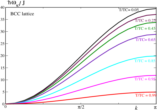
Figure 1: Dispersion relations, obtained by the CGF method, with wave vector (0,0,k) and without magnetic field.

It can be seen that $\omega_{\mathbf{k}}$, which includes magnon-magnon interactions, is strongly dependent on temperature. At temperatures near the critical value, the SW softening is clearly seen. A favorable comparison of these curves obtained by the CSD method with those rendered by the numerical LLE method was presented in Ref. (citenamefontU. Atxitia, D. Hinzke, O. Chubykalo-Fesenko, U. Nowak, H. Kachkachi, O. N. Mryasov, R. F. Evans, R. W. Chantrell, 2010).

Now, we present the magnetization curves, as a function of temperature and applied field, computed with the different methods for the bcc lattice and iron parameters (per atom) $J=1.44\>10^{-21}{\rm J}$ and $K=5.4\>10^{-24}{\rm J}$.

In Fig. 2, we plot the magnetization $m=\left\langle S^{z}\right\rangle/S$ as a function of (reduced) temperature $\tau=k_{\mathrm{B}}T/J_{0}$ in zero magnetic field, as obtained from i) QGF with two values of the nominal spin $S=5/2,30$, from ii) CGF, and from iii) classical MFT (CMFT), i.e. Eq. (54). We see that as $S$ increases the magnetization curve $m$ tends to that rendered by CGF and CMFT. In particular, at low temperature we do see the evolution from the $m\sim T^{3/2}$ Bloch law to the linear law $m\sim T$, as is typical of the classical Dirac-Heisenberg model. It is interesting how the CMFT result agrees with that of CGS when $m$ is plotted against the reduced temperature. The low-temperature asymptote (30) shows a good agreement with the QGF curve for $T\lesssim T_{\mathrm{C}}/4$. Similarly, the asymptote in the critical region (38) also reproduces correctly the QGF curve.

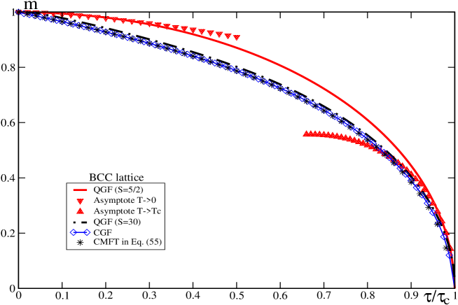
Figure 2: Magnetization against reduced temperature. Comparison of i) QGF for $S=5/2,30$, ii) CGF, and iii) classical MFT. We also show the low-temperature asymptote (30) and the asymptote near the critical temperature (38). The critical temperature $\tau_{c}$ is that of the method used for obtaining the corresponding magnetization curve and $\tau\equiv k_{B}T/J_{0}$.

In Fig. 3, we compare the magnetization curves rendered by CGF [see Eq. (52)] for various decoupling schemes, with MC as a benchmark. Here, we prefer to plot the magnetization against the absolute temperature $\tau$ so as to see how different are the critical values of temperature rendered by the various decoupling methods.

It is seen that the decoupling schemes of Callen and Swendsen agree quite well with MC. On the other hand, Copeland $\&$ Gersch (CG) and RPA decoupling schemes render nearly the same curve $m\left(\tau\right)$ that goes below the previous curves at high temperature. This is simply due to the fact that decoupling schemes with terms of high powers of $m$, e.g. $3$ in the CG decoupling and in the second term in Swendsen’s decoupling [see Eq. (10)], lead to a negligible contribution at temperatures nearing the critical value. On the contrary, contributions that are linear in $m$ in the decoupling schemes, such as Callen’s and Swendsen’s, do improve the magnetization curve at all temperatures.

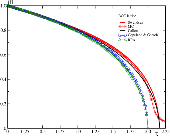
Figure 3: Magnetization curves rendered by different decoupling schemes. The methods are compared to Monte Carlo.

In Fig. 4, we compare the magnetization rendered by i) CGF and its Langevin function in Eq. (52) and ii) CSD given by Eq. (64), within RPA, and the two results are compared to MC. Globally, CGF renders a magnetization curve that keeps closer to MC than CSD method, which does so only at low temperature and near the critical temperature.

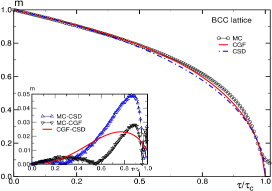
Figure 4: Magnetization obtained by CGF and CSD within RPA. The two methods are compared to Monte Carlo. Inset: difference between CGF, CSD (with RPA decoupling) and MC.

In the inset we plot the three differences between the CSD, CGF, and MC. It is seen that large deviations occur for $T/T_{C}\gtrsim 0.4$.

In Fig. 5 we compare, for the simpler case of an sc lattice, the classical Green’s function method with three decoupling schemes, with the numerical LLE method. It is seen that LLE compares quite well with CGF using the Swendson decoupling in almost the whole range of temperature. Note however, that in the numerical LLE method the finite-size effects are clearly seen in the critical temperature region, as is also the case with MC, while the analytical methods do not ignore such effects for they implicitly consider an infinite lattice.

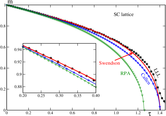
Figure 5: Comparison between the GF methods, the CSD method with RPA decoupling, the LLE approach and the classical Green’s function for an SC lattice structure.

Next, we study the relative magnetization variation

$$\widetilde{\delta m}\left(T,H\right)=\frac{m(T,H)-m(T,0)}{1-m(T,0)}$$

as a function of the applied field for different values of temperature, without anisotropy. The results are shown in Fig. 6.

In the quantum-mechanical case, we may use the low-temperature asymptote (30) to get (in the absence of anisotropy)

$$\widetilde{\delta m}\left(T,H\right) \simeq 1-\frac{1}{\zeta\left(3/2\right)}Z{}_{3/2}\left(\frac{g\mu_{B}H}{k_{\mathrm{B}T}}\right).$$

This can also be seen within the quantum linear SW theory which renders exactly the same expression. It is clear from the behavior of $Z_{p}\left(x\right)$ that in the low-temperature regime $\widetilde{\delta m}$ decreases when the temperature increases.

In the classical case and at low temperature, we use the asymptote (57) and obtain

$$\widetilde{\delta m}{}^{\mathrm{CGF}} \simeq 1-\left(1+\kappa\right)\psi(1)+\left(1+\kappa\right)\psi(1)\left(\lambda^{\prime}-\psi(1)\right)P_{N}(\psi\left(1\right))\times\tau^{\prime}.$$

Here we see that this expression increases when the temperature increases since $\lambda^{\prime}=1/\left(1+\kappa\right)>\psi\left(1\right)=1/\left(h^{\prime}+\left(1+\kappa\right)\right)$ for any $h^{\prime}>0$.

However, it remains unclear why in the quantum-mechanical case there is a change of behavior at a particular temperature because it is difficult to derive an (approximate) analytical expression for the latter. Indeed, this would at least require to derive the magnetization asymptote in the critical region in finite magnetic field which, unfortunately, leads to a rather cumbersome expression. Nevertheless, quantum spin effects are attenuated at high temperatures and as such the quantum approach renders the same behavior for the magnetization as the classical one.

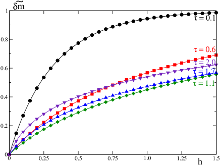
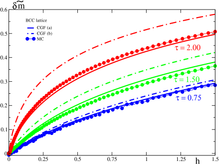
Figure 6: Field dependence of the relative magnetization variation $\widetilde{\delta m}$, (left) from QGF with RPA decoupling and (right) from CGF (Callen (a) and RPA (b) decoupling) and MC.

IV.2 SW spectrum and exchange stiffness at finite temperature

Now we discuss the exchange stiffness as a function of the magnetization taking account of nonlinear SW effects. As we have seen, taking account of these effects (or magnon-magnon interactions), through the various decoupling schemes, leads to a temperature-dependent dispersion. This dependence on temperature comes about through the magnetization $m$. Let us consider, for simplicity, the case with the sole contribution from exchange coupling. Hence, we may define the SW stiffness $D$ as follows

$$\hbar\omega_{\mathbf{k}}^{\prime}=D\left(m\right)\left(1-\gamma_{\mathbf{k}}\right),$$ (71)

assuming that all SW nonlinear effects [see the last term in e.g. Eqs. (13, III.2)] are booked into the function $D\left(m\right)$. On the other hand, in the absence of applied field and anisotropy, and for a given decoupling scheme with the parameter $\alpha$ introduced in Eq. (9) we deduce from Eq. (17) that

$$D\left(m\right)=J_{0}^{\prime}mQ^{\prime}\left(\alpha,m\right)$$

with

$$Q^{\prime}(\alpha,\beta)=1+\frac{\alpha}{\mathcal{N}}\sum_{\mathbf{p}}\frac{\gamma_{\mathbf{p}}}{\beta\hbar\omega_{\mathbf{p}}^{\prime}}$$

in the classical limit.

In the general case, as discussed in the previous sections, the dispersion $\omega_{\mathbf{k}}$ and the magnetization $m$ are solved for by using the system of coupled equations and then $D\left(m\right)$ is obtained by fitting the curves of $\omega$ as a function of the wave vector $\mathbf{k}$ in a given direction in Fourier space. Next, we substitute $\hbar\omega_{\mathbf{k}}^{\prime}=J_{0}^{\prime}mQ^{\prime}\left(1-\gamma_{\mathbf{k}}\right)$ in $Q^{\prime}$ to obtain

$$Q^{\prime}\left(\alpha,\beta\right)=1+\frac{1}{Q^{\prime}\left(\alpha,\beta\right)}\frac{\alpha/m}{\mathcal{N}}\sum_{\mathbf{p}}\frac{\gamma_{\mathbf{p}}}{1-\gamma_{\mathbf{k^{\prime}}}}\times\tau^{\prime}=1+\frac{\alpha\left(W-1\right)}{mQ^{\prime}\left(\alpha,\beta\right)}\times\tau^{\prime}$$ (72)

where $W$ is the Watson integral for the given lattice.

At low temperature, the magnetization is given by (CGF or CSD)

$$m\simeq 1-\frac{W}{Q^{\prime}\left(\alpha,\beta\right)}\tau^{\prime}$$

leading to

$$\tau^{\prime}=\left(1-m\right)\frac{Q^{\prime}}{W}.$$

Then, when this is substituted in Eq. (72) yields

$$Q^{\prime}\left(\alpha,\beta\right)=1+\frac{W-1}{W}\times\frac{\left(1-m\right)\alpha}{m}$$

and thereby the spin stiffness $D\left(m\right)$ reads

$$D\left(m\right)=J_{0}^{\prime}m\left[1+\frac{W-1}{W}\times\frac{\left(1-m\right)\alpha}{m}\right].$$ (73)

Now, defining $\phi=\alpha\left(m\right)/m$ and $\varsigma\equiv\left(W-1\right)/W$, we write

$$D\left(m\right)=J_{0}^{\prime}m\left[1+\varsigma\phi\left(m\right)\times\left(1-m\right)\right].$$

Finally, considering the fact that at low temperature $1-m$ is small so that we may write

$$D\left(m\right)\simeq J_{0}^{\prime}m\left[1-\left(1-m\right)\right]^{-\varsigma\phi\left(m\right)}=m^{1-\varsigma\phi\left(m\right)}.$$

$\alpha\left(m\right)$ and thereby $\phi\left(m\right)$ is given according to the RPA, Callen’s, Copeland and Gersch or Swendsen decoupling scheme, see Eq. (10) et seq. For the RPA decoupling, for instance, $\alpha=0$ and thus $D\left(m\right)\sim m$, as it should. For Callen’s decoupling, $\alpha\left(m\right)=m$ leading to $D\left(m\right)\sim m^{1-\varsigma}$. For a decoupling scheme with $\alpha\left(m\right)=am+bm^{3}$ we make an expansion around $m\simeq 1$ and obtain $D\left(m\right)\simeq m\left[1-\zeta\left(a+b\right)\left(m-1\right)\right]$.

In Fig. 7 we plot the exchange stiffness as obtained numerically from Eq. (71) and Eqs. (13, III.2), for the decoupling schemes discussed in Fig. 3.

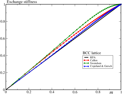
Figure 7: Exchange stiffness against the magnetization for different decoupling schemes obtained by CGF.

As is seen in Eq. (73) and confirmed by the numerical results in Fig. 7, the exchange stiffness depends on the decoupling scheme or the way the spin-spin correlations are tackled, especially at moderate temperatures. Obviously, the curves corresponding to the four decoupling schemes merge for $m\sim 1$ (very low temperature) and $m\sim 0$, i.e. at high temperature where they exhibit a linear behavior.

V Conclusion

We have established clear connections between the quantum/classical Green function technique and the classical spectral density method, and have compared them with the numerical methods of Monte Carlo and Landau-Lifshitz-Langevin dynamics. We have proposed a unified decoupling scheme for both anisotropy and exchange contributions, for classical as well as for quantum spins which allows us to establish a clear connection between the various methods and to obtain reasonable results for the magnetization and critical temperature. We have computed the spin-wave spectrum at finite temperature and inferred the magnetization as a function of temperature and field and have obtained the exchange stiffness, for various decoupling schemes. Asymptotic expressions for the magnetization have been given at low temperature and in the critical region, both for classical and quantum spins, and the crossover between them has been established. As far as the (semi-)analytical methods are concerned, it turns out that the classical Green’s function technique is more straightforward and does not require any a priori assumptions about the the system’s spectral density. In particular, Callen’s famous formula for the magnetization is recast in a compact form using the Brillouin function. This makes it straightforward to obtain the classical limit leading to the familiar Langevin function for the magnetization. However, the outcome is still a transcendental equation involving the spin-wave density, unlike the Langevin form one obtains from mean-field theory.

In future work, we would like to extend the present calculations and the Green’s function technique to finite-size systems by taking account of boundary and surface effects, similarly to what has been done in Refs. (citenamefontH. Kachkachi and D. A. Garanin, 2001natexlaba; citenamefontH. Kachkachi and D.A. Garanin, 2001). This should be useful for studying the dynamics of multi-layered magnetic systems and magnetic nanostructures.

VI Acknowledgement

RB and HK acknowldge financial support from the French National Research Agency under the program ANR Jeunes-Chercheurs MARVEL. UA and OCF acknowledge funding by the Spanish Ministry of Science and Innovation under the grant FIS2010-20979-C02-02.

Appendix A Quantum Green Function Method

In this section we briefly describe the quantum Green function method (QGM) in the case of an oblique magnetic field.

In order to compute the spin-wave (SW) spectrum and the magnetization, one deals with the spin fluctuations with respect to the equilibrium configuration, which has to be determined beforehand. In practice, one assumes that there exists a net direction of the system’s magnetization denoted by $\mathbf{e}_{3}$

$$\mathbf{m}=\frac{1}{\mathcal{N}}\sum_{i}\mathbf{S}_{i}\equiv m\,\mathbf{e}_{3}.$$

We start by passing to the new coordinate system in which the (usually adopted) $z$ reference direction is now the direction $\mathbf{e}_{3}$. This amounts to performing a rotation of the original variables $\mathbf{S}_{i}$ to the new ones $\bm{\sigma}_{i}$ around a given axis and at a given angle depending on $\mathbf{e}_{3}$. Following the standard approach (citenamefontM. G. Pini, P. Politi, and R. L. Stamps, 2005; citenamefontP. Frobrich, P.J. Kuntz, 2006; citenamefontS. Schwieger, J. Kienert, and W. Nolting, 2005), we use the Holstein-Primakov representation for the new variables $\bm{\sigma}_{i}$ . To rewrite the Green’s functions in the local reference frame, we use a rotation matrix $\mathcal{R}(\mathbf{e}_{y},\vartheta)$ for the rotation of an angle $\vartheta$ around the axis $\mathbf{e}_{y}$. So in the Hamiltonian (1) we replace the spin variable $\mathbf{S}_{i}$ by the new one $\bm{\sigma}_{i}$ (with $\left\|\bm{\sigma}_{i}\right\|=\left\|\mathbf{S}_{i}\right\|=S$) using

$$\mathbf{S}_{i} =\mathcal{R}(\mathbf{e}_{y},-\vartheta)\bm{\sigma}_{i}=\cos\vartheta\,\bm{\sigma}_{i}-\sin\vartheta\,(\bm{\sigma}_{i}\times\mathbf{e}_{y})+\left(1-\cos\vartheta\right)(\bm{\sigma}_{i}\cdot\mathbf{e}_{y})\mathbf{e}_{y}.$$ (74)

For instance,

$$S^{z}=\cos\vartheta\sigma_{i}^{z}-\sin\vartheta\sigma_{i}^{x}$$

and the Zeeman term ($H_{y}=0$) becomes

$$\mathbf{S}_{i}\cdot\mathbf{H}=\left[H^{x}\cos\vartheta-H^{z}\sin\vartheta\right]\sigma_{i}^{x}+\left[H^{z}\cos\vartheta+H^{x}\sin\vartheta\right]\sigma_{i}^{z}.$$ (75)

We also define the rotated field

$$\mathbf{H}_{\mathcal{R}}\equiv\mathcal{R}(\mathbf{e}_{y},\vartheta)\mathbf{H}.$$

The new spin variables satisfy the same algebra as the original spin variables $\mathbf{S}_{i}$, i.e.,

$$\left[\sigma_{i}^{+},\,\sigma_{j}^{-}\right] = 2\delta_{ij}\,\sigma_{i}^{3}$$

$$\left[\sigma_{i}^{3},\,\sigma_{j}^{\mu}\right] = \mu\sigma_{i}^{\mu}\delta_{ij},\qquad\mu=\pm.$$ (76)

Then, rewriting the Hamiltonian (1) in the new variables, we obtain the quadratic form

$$\mathcal{H} = -\frac{1}{2}\sum_{i,j=1}^{\mathcal{N}}\sum_{\mu,\nu=+,-,(3)}\sigma_{i}^{\mu}Q_{ij}^{\mu\nu}\sigma_{j}^{\nu}-{\displaystyle{\displaystyle\sum_{i=1}^{\mathcal{N}}}}{\displaystyle{\displaystyle\sum_{\mu=+,-,(3)}}}L^{\mu}\sigma_{i}^{\mu}$$ (77)

with the linear coefficients

$$L^{+}=\left(g\mu_{B}\right)\frac{H_{\mathcal{R}}^{-}}{2},\qquad L^{-}=\left(g\mu_{B}\right)\frac{H_{\mathcal{R}}^{+}}{2},\qquad L^{3}=\left(g\mu_{B}\right)H_{\mathcal{R}}^{3}$$ (78)

and the quadratic ones

$$\begin{array}[]{ll}Q_{ij}^{++}=\frac{K}{2}\sin^{2}\vartheta\,\delta_{ij}=Q_{ij}^{--},&Q_{ij}^{+-}=\frac{1}{2}\left[J_{ij}+K\sin^{2}\vartheta\delta_{ij}\right]=Q_{ij}^{-+},\\ \\ Q_{ij}^{33}=J_{ij}+2K\cos^{2}\vartheta\delta_{ij}&Q_{ij}^{3+}=Q_{ij}^{+3}=-K\sin\vartheta\cos\vartheta\delta_{ij}=Q_{ij}^{3-}=Q_{ij}^{-3}.\end{array}$$ (79)

These satisfy the symmetry relation $Q_{ij}^{\mu\nu}=Q_{ji}^{\mu\nu}$.

Applying the RPA decoupling to a homogeneous ferromagnet, i.e. with $\left\langle\sigma_{i}^{3}\right\rangle=\left\langle\sigma^{3}\right\rangle$, we obtain the following (coupled) equations for the relevant GFs after Fourier transformations with respect to time and space

$$\left(\begin{array}[]{lll}\omega-\mathcal{A}_{\mathbf{k}}&\mathcal{B}_{\mathbf{k}}&2\mathcal{A}_{\mathbf{k}}^{-}\left(\mathcal{K}_{\sigma}\right)\\ -\mathcal{B}_{\mathbf{k}}&\omega+\mathcal{A}_{\mathbf{k}}&-2\mathcal{A}_{\mathbf{k}}^{+}\left(\mathcal{K}_{\sigma}\right)\\ \mathcal{A}_{\mathbf{k}}^{+}\left(\mathcal{K}_{\sigma}/2\right)&-\mathcal{A}_{\mathbf{k}}^{-}\left(\mathcal{K}_{\sigma}/2\right)&\omega\end{array}\right)\left(\begin{array}[]{l}\mathcal{G}_{\mathbf{k}}^{+-}\\ \mathcal{G}_{\mathbf{k}}^{--}\\ \mathcal{G}_{\mathbf{k}}^{3-}\end{array}\right)=\left(\begin{array}[]{l}2\left\langle\sigma^{3}\right\rangle\\ 0\\ 0\end{array}\right)$$ (80)

where

$$\begin{array}[]{lll}\mathcal{A}_{\mathbf{k}}&\equiv&L^{3}+\mathcal{K}_{\sigma}\left\langle\sigma^{3}\right\rangle\left(2\cos^{2}\vartheta-\sin^{2}\vartheta\right)+J_{0}\left\langle\sigma^{3}\right\rangle\left(1-\gamma_{\mathbf{k}}\right),\\ \mathcal{A}_{\mathbf{k}}^{\pm}&\equiv&L^{\pm}-\mathcal{K}_{\sigma}\left\langle\sigma^{3}\right\rangle\sin 2\vartheta,\\ \mathcal{B}_{\mathbf{k}}&\equiv&\mathcal{K}_{\sigma}\left\langle\sigma^{3}\right\rangle\sin^{2}\vartheta.\end{array}$$ (81)

$J_{0}$ is the $\mathbf{k}=0$ component of the exchange coupling given by

$$J_{0}\equiv J\left(\text{0}\right)=\sum_{j}J_{ij}=zJ$$ (82)

with $z$ being the coordination number. If the exchange is isotropic, we may write

$$J\left(\mathbf{k}\right) =J\left(-\mathbf{k}\right)=\sum_{j}e^{-i\mathbf{k}\cdot\mathbf{r}_{ij}}J_{ij}=J_{0}\times\frac{1}{z}\sum_{j}e^{-i\mathbf{k}\cdot\mathbf{r}_{ij}}\equiv J_{0}\gamma_{\mathbf{k}}.$$ (83)

For a bcc lattice we have ($z=8$) the unit cell unit vectors

$$\mathbf{\delta}_{ij}\equiv\frac{a}{2}\left(\pm\mathbf{e}_{{}_{x}},\pm\mathbf{e}_{y},\pm\mathbf{e}_{z}\right)$$

and thereby

$$\gamma_{\mathbf{k}} = \cos\frac{ak_{x}}{2}\cos\frac{ak_{y}}{2}\cos\frac{ak_{z}}{2},$$ (84)

$a$ being the lattice parameter. For long wavelength excitations we use $\cos k_{\alpha}\simeq 1-\frac{1}{2}k_{\alpha}^{2}$, which yields

$$1-\gamma_{\mathbf{k}} \simeq \left(ak\right)^{2}.$$

Note that the EM for $\mathcal{G}_{ij}^{z-}$, that is the last equation in the system (80), provides the equilibrium configuration. Near equilibrium, the net magnetic moment $\mathbf{m}=\frac{1}{\mathcal{N}}\sum_{i}\mathbf{\sigma}_{i}$ does not change much, which means that $d\mathbf{m}/dt\simeq 0$. In quantum mechanics, this implies that the total magnetic moment along the equilibrium direction commutes with the Hamiltonian, or in other words, the projection of the total magnetic moment along the equilibrium direction is conserved, that is

$$i\frac{d}{dt}\left(\frac{1}{\mathcal{N}}\sum_{i}\sigma_{i}^{3}\right)=\left[\frac{1}{\mathcal{N}}\sum_{i}\sigma_{i}^{3},\mathcal{H}\right]=0.$$ (85)

On the other hand, on the same level of approximation as that used to obtain the system of EM (80), the commutator above reads

$$\left[\frac{1}{\mathcal{N}}\sum_{i}\sigma_{i}^{3},\mathcal{H}\right] \simeq\left[\left(g\mu_{B}\right)\left(H^{z}\sin\vartheta-H^{x}\cos\vartheta\right)+\mathcal{K}\left\langle\sigma^{3}\right\rangle\sin 2\vartheta\right]\times\frac{1}{\mathcal{N}}\sum_{i}\left(i\sigma_{i}^{y}\right),$$ (86)

which, if set to zero according to (85), leads to the equilibrium condition

$$\left(h^{z}\sin\vartheta-h^{x}\cos\vartheta\right)+\mathcal{K}_{\sigma}\left\langle\sigma^{3}\right\rangle\sin 2\vartheta=0.$$ (87)

Hence, the GF $\mathcal{G}_{\mathbf{k}}^{z-}(\omega)$ is eliminated from the system (80) and thereby the latter simplifies into the following system of two coupled equations

$$\left\{\begin{array}[]{ccc}\left(\omega-\mathcal{A}_{\mathbf{k}}\right)\mathcal{G}_{\mathbf{k}}^{+-}+\mathcal{B}_{\mathbf{k}}\mathcal{G}_{\mathbf{k}}^{--}&=&2\left\langle\sigma^{3}\right\rangle\\ \\ -\mathcal{B}_{\mathbf{k}}\mathcal{G}_{\mathbf{k}}^{+-}+\left(\omega+\mathcal{A}_{\mathbf{k}}\right)\mathcal{G}_{\mathbf{k}}^{--}&=&0.\end{array}\right.$$ (88)

Appendix B Decoupling of exchange contributions within CSD

Following the procedure described in section III.3, before Eq. (62), we obtain

$$\frac{1}{\mathcal{N}}\sum_{\mathbf{q}}J_{\mathbf{\mathbf{q}}}^{\prime}\begin{array}[]{c}\left\langle\left\{s_{\mathbf{k}-\mathbf{q}}^{z}(\tau)s_{\mathbf{q}}^{+}(\tau);s_{-\mathbf{k}}^{-}(0)\right\}\right\rangle_{\omega}\end{array} \simeq mJ_{\mathbf{k}}^{\prime}\left\langle\left\langle s_{\mathbf{k}}^{+}(\tau);s_{-\mathbf{k}}^{-}\right\rangle\right\rangle_{\omega}$$

$$-\frac{m}{\mathcal{N}^{2}}\sum_{\mathbf{p},\mathbf{q}}J_{\mathbf{\mathbf{q}}}^{\prime}\frac{\left\langle s_{\mathbf{p}}^{+}s_{\mathbf{q}}^{-}\right\rangle}{2}\left\langle\left\langle s_{\mathbf{k}-\mathbf{p}-\mathbf{q}}^{+}(\tau);s_{-\mathbf{k}}^{-}\right\rangle\right\rangle_{\omega}.$$

Similarly, for the second contribution we get

$$\frac{1}{\mathcal{N}}\sum_{\mathbf{q}}J_{\mathbf{\mathbf{q}}}^{\prime}\left\langle\left\{s_{\mathbf{q}}^{z}(\tau)s_{\mathbf{k}-\mathbf{q}}^{+}(\tau);s_{-\mathbf{k}}^{-}(0)\right\}\right\rangle_{\omega} \simeq mJ_{\mathbf{\mathbf{0}}}^{\prime}\left\langle\left\langle s_{\mathbf{k}}^{+}(\tau);s_{-\mathbf{k}}^{-}\right\rangle\right\rangle_{\omega}$$

$$-\frac{m}{\mathcal{N}^{2}}\sum_{\mathbf{p},\mathbf{q}}J_{\mathbf{\mathbf{q}}}^{\prime}\frac{\left\langle s_{\mathbf{p}}^{+}s_{\mathbf{k}-\mathbf{q}}^{-}\right\rangle}{2}\left\langle\left\langle s_{\mathbf{q}-\mathbf{p}}^{+}(\tau);s_{-\mathbf{k}}^{-}\right\rangle\right\rangle_{\omega}.$$

Now, using the two moment equations

$$\left\{\begin{array}[]{lll}\intop_{-\infty}^{\infty}\frac{d\omega}{2\pi}\Lambda_{\mathbf{k}}\left(\omega\right)=i\left\langle\left\{S_{\mathbf{k}}^{+},S_{-\mathbf{k}}^{-}\right\}\right\rangle,\\ \\ \intop_{-\infty}^{\infty}\frac{d\omega}{2\pi}\omega\Lambda_{\mathbf{k}}\left(\omega\right)=-\left\langle\left\{\left\{S_{\mathbf{k}}^{+},\mathcal{H}\right\},S_{-\mathbf{k}}^{-}\right\}\right\rangle.\end{array}\right.$$ (89)

with the spectral density, see Ref. citenamefontA. Cavallo, F. Cosenza, and L. De Cesare (2005)

$$\Lambda_{\mathbf{k}}\left(\omega\right)=\left\langle\left\langle s_{\mathbf{k}}^{+}(\tau);s_{-\mathbf{k}}^{-}\right\rangle\right\rangle_{\omega}=i\left\langle\left\{s_{\mathbf{k}}^{+}\left(\tau\right),s_{-\mathbf{k}}^{-}\left(0\right)\right\}\right\rangle_{\omega}=2\pi\mathcal{N}m\delta\left(\omega-\omega_{\mathbf{k}}\right)$$ (90)

we integrate over $\omega$ and obtain for the first contribution

$$\intop_{-\infty}^{\infty}\frac{d\omega}{2\pi}\frac{1}{\mathcal{N}}\sum_{\mathbf{q}}J_{\mathbf{\mathbf{q}}}^{\prime}\begin{array}[]{c}\left\langle\left\{s_{\mathbf{k}-\mathbf{q}}^{z}(\tau)s_{\mathbf{q}}^{+}(\tau);s_{-\mathbf{k}}^{-}(0)\right\}\right\rangle_{\omega}\end{array} \simeq 2\mathcal{N}m^{2}J_{\mathbf{k}}^{\prime}-\frac{2m}{\mathcal{N}}\sum_{\mathbf{q}}J_{\mathbf{\mathbf{q}}}^{\prime}\left\langle s_{-\mathbf{q}}^{+}s_{\mathbf{q}}^{-}\right\rangle$$

and for the second

$$\intop_{-\infty}^{\infty}\frac{d\omega}{2\pi}\frac{1}{\mathcal{N}}\sum_{\mathbf{q}}J_{\mathbf{\mathbf{q}}}^{\prime}\left\langle\left\{s_{\mathbf{q}}^{z}(\tau)s_{\mathbf{k}-\mathbf{q}}^{+}(\tau);s_{-\mathbf{k}}^{-}(0)\right\}\right\rangle_{\omega} \simeq 2\mathcal{N}m^{2}J_{\mathbf{\mathbf{0}}}^{\prime}-\frac{m^{2}}{\mathcal{N}}\sum_{\mathbf{q}}J_{\mathbf{\mathbf{q}}}^{\prime}\left\langle s_{\mathbf{q}-\mathbf{k}}^{+}s_{\mathbf{k}-\mathbf{q}}^{-}\right\rangle.$$

Then, subtracting the second contribution from the first yields

$$\intop_{-\infty}^{\infty}\frac{d\omega}{2\pi}\frac{1}{\mathcal{N}}\sum_{\mathbf{q}}J_{\mathbf{\mathbf{q}}}^{\prime}\left[\begin{array}[]{c}\left\langle\left\{s_{\mathbf{k}-\mathbf{q}}^{z}(\tau)s_{\mathbf{q}}^{+}(\tau);s_{-\mathbf{k}}^{-}(0)\right\}\right\rangle_{\omega}\\ -\left\langle\left\{s_{\mathbf{q}}^{z}(\tau)s_{\mathbf{k}-\mathbf{q}}^{+}(\tau);s_{-\mathbf{k}}^{-}(0)\right\}\right\rangle_{\omega}\end{array}\right] \simeq 2\mathcal{N}m^{2}\left(J_{\mathbf{k}}^{\prime}-J_{\mathbf{\mathbf{0}}}^{\prime}\right)-\frac{m^{2}}{\mathcal{N}}\sum_{\mathbf{q}}\left(J_{\mathbf{\mathbf{q}}}^{\prime}-J_{\mathbf{\mathbf{k}}-\mathbf{\mathbf{q}}}^{\prime}\right)\left\langle s_{-\mathbf{q}}^{+}s_{\mathbf{q}}^{-}\right\rangle.$$

On the other hand, using the zero-moment equation, we get

$$\intop_{-\infty}^{\infty}\frac{d\omega}{2\pi}\frac{1}{\mathcal{N}}\sum_{\mathbf{q}}J_{\mathbf{\mathbf{q}}}^{\prime}\left[\begin{array}[]{c}\left\langle\left\{s_{\mathbf{k}-\mathbf{q}}^{z}(\tau)s_{\mathbf{q}}^{+}(\tau);s_{-\mathbf{k}}^{-}(0)\right\}\right\rangle_{\omega}\\ -\left\langle\left\{s_{\mathbf{q}}^{z}(\tau)s_{\mathbf{k}-\mathbf{q}}^{+}(\tau);s_{-\mathbf{k}}^{-}(0)\right\}\right\rangle_{\omega}\end{array}\right] =-\frac{1}{\mathcal{N}}\sum_{\mathbf{q}}\left(J_{\mathbf{\mathbf{q}}}^{\prime}-J_{\mathbf{\mathbf{k}}-\mathbf{\mathbf{q}}}^{\prime}\right)\left[2\left\langle s_{\mathbf{q}}^{z}s_{-\mathbf{q}}^{z}\right\rangle+\left\langle s_{-\mathbf{q}}^{-}s_{\mathbf{q}}^{+}\right\rangle\right].$$

Consequently, we have the equation

$$2\mathcal{N}m^{2}\left(J_{\mathbf{\mathbf{0}}}^{\prime}-J_{\mathbf{k}}^{\prime}\right)+\frac{m^{2}}{\mathcal{N}}\sum_{\mathbf{q}}\left(J_{\mathbf{\mathbf{q}}}^{\prime}-J_{\mathbf{\mathbf{k}}-\mathbf{\mathbf{q}}}^{\prime}\right)\left\langle s_{-\mathbf{q}}^{+}s_{\mathbf{q}}^{-}\right\rangle\simeq\frac{1}{\mathcal{N}}\sum_{\mathbf{q}}\left(J_{\mathbf{\mathbf{q}}}^{\prime}-J_{\mathbf{\mathbf{k}}-\mathbf{\mathbf{q}}}^{\prime}\right)\left[2\left\langle s_{\mathbf{q}}^{z}s_{-\mathbf{q}}^{z}\right\rangle+\left\langle s_{-\mathbf{q}}^{-}s_{\mathbf{q}}^{+}\right\rangle\right]$$

which leads to

$$\sum_{\mathbf{q}}\left(J_{\mathbf{\mathbf{q}}}^{\prime}-J_{\mathbf{\mathbf{k}}-\mathbf{\mathbf{q}}}^{\prime}\right)\left\langle s_{\mathbf{q}}^{z}s_{-\mathbf{q}}^{z}\right\rangle\simeq\mathcal{N}^{2}m^{2}\left(J_{\mathbf{\mathbf{0}}}^{\prime}-J_{\mathbf{k}}^{\prime}\right)+\frac{1}{2}m^{2}\sum_{\mathbf{q}}\left(J_{\mathbf{\mathbf{q}}}^{\prime}-J_{\mathbf{\mathbf{k}}-\mathbf{\mathbf{q}}}^{\prime}\right)\left\langle s_{-\mathbf{q}}^{+}s_{\mathbf{q}}^{-}\right\rangle-\frac{1}{2}\sum_{\mathbf{q}}\left(J_{\mathbf{\mathbf{q}}}^{\prime}-J_{\mathbf{\mathbf{k}}-\mathbf{\mathbf{q}}}^{\prime}\right)\left\langle s_{-\mathbf{q}}^{-}s_{\mathbf{q}}^{+}\right\rangle.$$

One can can easily check that $\left\langle s_{-\mathbf{q}}^{+}s_{\mathbf{q}}^{-}\right\rangle=\left\langle s_{-\mathbf{q}}^{-}s_{\mathbf{q}}^{+}\right\rangle$ and thereby one obtains

$$\sum_{\mathbf{q}}\left(J_{\mathbf{\mathbf{q}}}^{\prime}-J_{\mathbf{\mathbf{k}}-\mathbf{\mathbf{q}}}^{\prime}\right)\left\langle s_{\mathbf{q}}^{z}s_{-\mathbf{q}}^{z}\right\rangle\simeq\sum_{\mathbf{q}}\left(J_{\mathbf{\mathbf{q}}}^{\prime}-J_{\mathbf{\mathbf{k}}-\mathbf{\mathbf{q}}}^{\prime}\right)\left[\mathcal{N}^{2}m^{2}\Delta\left(\mathbf{q}\right)-\frac{1}{2}\left(1-m^{2}\right)\left\langle s_{\mathbf{q}}^{+}s_{-\mathbf{q}}^{-}\right\rangle\right].$$

This may also be recast into the form (62) which can be more easily compared to RPA.

Appendix C The critical temperature via different approaches.

Within the QGF approach and using parameter $\phi$ for exchange decoupling, the Curie temperature can be calculated from Eq. (43) by setting $\left\langle\sigma^{3}\right\rangle\simeq 0$ at $\tau=\tau_{c}$. This leads to [see Eq. (33) for notation]

$$\tau_{c}=\frac{S(S+1)}{3}\frac{\kappa+Q(\phi,\tau_{c})}{P(\Lambda)}.$$

In the absence of anisotropy, which is negligible near $T_{c}$, we obtain

$$\tau_{c}^{\mathrm{QGF}}=\frac{S(S+1)}{3}\frac{Q_{\mathrm{exch}}(\phi,\tau_{c}^{\mathrm{QGF}})}{W}\rightarrow\tau_{c}^{\mathrm{QGF}}=\frac{S\left(S+1\right)}{3W}\left[1+\frac{\phi}{3}\left(1+\frac{1}{S}\right)\left(1-\frac{1}{W}\right)\right].$$ (91)

In CGF (or in CSD where we obtain the same result), we similarly use the high-temperature asymptote (60) and obtain

$$\tau_{c}^{\mathrm{CGF}}=S^{2}\frac{Q_{\mathrm{exch}}^{\prime}(\phi,\tau_{c}^{\mathrm{CGF}})}{3W}\rightarrow\tau_{c}^{\mathrm{CGF}}=\frac{S^{2}}{3W}\left[1+\frac{\phi}{3}\left(1-\frac{1}{W}\right)\right].$$ (92)

We remark in passing that this is also the result that one obtains within the spherical model, in the isotropic case (citenamefontH. Kachkachi and D. A. Garanin, 2001natexlaba), i.e. $\kappa=0$, and for a RPA decoupling $\phi=0$, which yields

$$\tau_{c}=\frac{1}{W}\frac{S^{2}}{3}.$$ (93)

On the other hand, from the MFT magnetization (54) one obtains the Curie temperature (for $H=0$ and $\kappa=0$)

$$\tau_{C}^{\mathrm{MFT}}=\frac{J_{0}S^{2}}{3}.$$ (94)

Note that contrary to the MFT result (94), the expression (92) for $\tau_{C}$, as obtained from the GF in the classical limit, or Eq. (93) from the isotropic spherical model, depends on the lattice and on the SW dispersion via the Watson integral $W$. Moreover, as mentioned earlier, we can relate MFT to SWT by assuming that all excitations are degenerate and by ignoring spin fluctuations. More precisely, this amounts to dropping the terms that are responsible for the propagation of the SWs (or magnons) through the lattice. This can be done by dropping the propagation function $\gamma_{\mathbf{k}}$ from all SWT expressions. Hence, the MFT result (94) can be obtained from the classical limit of the GF result (92) by formally setting $\gamma_{\mathbf{k}}=0$ in the lattice integral $W$ (leading to $W=1$) and taking $\phi=0$.

In Table 1 we collect the values of $\tau_{C}$ estimated by the different approaches in the isotropic case. First, we remark that the values obtained within quantum-mechanical approaches are higher than the classical ones. Indeed, comparing for instance Eqs. (91) and (92) we see that for small spin values the difference in $\tau_{c}$, due to the contribution $S$ in $S\left(S+1\right)=S^{2}+S$, is non negligible. This is no surprise because this decoupling scheme, unlike RPA, accounts for magnon-magnon interactions whose role becomes crucial in the vicinity of the critical temperature. Second, there is a perfect agreement between the two classical methods CGF and CSD. As discussed earlier, this shows that given that i) CGF renders the same results as CSD and ii) that CGF does not require any assumptions about the spectral function, it might be preferable to use the CGF method.

Method	$\begin{array}[]{ccc}&\mbox{QGF}&\mathrm{}\\ \mathrm{(a)}&\mathrm{(b)}&\mathrm{(c)}\end{array}$	$\begin{array}[]{ccc}&\mbox{CGF}&\mathrm{}\\ \mathrm{(a)}&\mathrm{(b)}&\mathrm{(c)}\end{array}$	$\begin{array}[]{ccc}&\mbox{CSD}&\mathrm{}\\ \mathrm{(a)}&\mathrm{(b)}&\mathrm{(c)}\end{array}$	MFT	MC
$\tau_{\mathrm{C}}/S^{2}$ (K)	$\begin{array}[]{cccc}0.335&0.380&&0.354\end{array}$	$\begin{array}[]{ccc}0.240&0.262&0.262\end{array}$	$\begin{array}[]{ccc}0.240&0.262&0.262\end{array}$	$0.333$	$0.268$

Table 1: Reduced Curie temperature $\tau_{\mathrm{C}}/S^{2}\equiv k_{\mathrm{B}}T_{\mathrm{C}}/S^{2}J_{0}$ for a bcc lattice with Fe parameters and $S=5/2$. (a) stands for the RPA or Copeland-Gersch, (b) for Callen, and (c) for Swenden’s decoupling schemes used for the exchange contributions.

References

- citenamefontR. E. Rottmayer et al. (2006) R. E. Rottmayer et al., IEEE Trans. Magn. 42, 2417 (2006).
- citenamefontU. Atxitia, O. Chubykalo-Fesenko, N. Kazantseva, D. Hinzke, U. Nowak, and R. W. Chantrell (2007) U. Atxitia, O. Chubykalo-Fesenko, N. Kazantseva, D. Hinzke, U. Nowak, and R. W. Chantrell, Appl. Phys. Lett. 91, 232507 (2007).
- citenamefontI. L. Prejbeanu, M. Kerekes, R. C. Sousa, O. Redon, B. Dieny, and J.P.Nozeires (2007) I. L. Prejbeanu, M. Kerekes, R. C. Sousa, O. Redon, B. Dieny, and J.P.Nozeires, J. Phys.: Condens. Mat. 19, 165218 (2007).
- citenamefontD. Hinzke and U. Nowak (2011) D. Hinzke and U. Nowak, Phys. Rev. Lett. 107, 027205 (2011).
- citenamefontN. Kazantseva, D. Hinzke, U. Nowak, R. W. Chantrell, U. Atxitia, and O. Chubykalo-Fesenko (2008) N. Kazantseva, D. Hinzke, U. Nowak, R. W. Chantrell, U. Atxitia, and O. Chubykalo-Fesenko, Phys. Rev. B 77, 184428 (2008).
- citenamefontO.A.Chubykalo, J.D.Hannay, M.A.Wongsam, R.W.Chantrell and J.M.Gonzalez (2002) O.A.Chubykalo, J.D.Hannay, M.A.Wongsam, R.W.Chantrell y J.M.Gonzalez, Phys. Rev. B 65, 184428 (2002).
- citenamefontU. Atxitia, D. Hinzke, O. Chubykalo-Fesenko, U. Nowak, H. Kachkachi, O. N. Mryasov, R. F. Evans, R. W. Chantrell (2010) U. Atxitia, D. Hinzke, O. Chubykalo-Fesenko, U. Nowak, H. Kachkachi, O. N. Mryasov, R. F. Evans, R. W. Chantrell, Phys. Rev. B 82, 134440 (2010).
- citenamefontW. F. Brown (1963) W. F. Brown, Phys. Rev. 135, 1677 (1963).
- citenamefontA. Lyberatos and R.W. Chantrell (1993) A. Lyberatos and R.W. Chantrell, J. Appl. Phys. 73, 6501 (1993).
- citenamefontBinder and Heermann (1992) K. Binder and D. Heermann, Monte Carlo simulation in statistical physics (Springer-Verlag, Berlin, 1992).
- citenamefontA. I. Akhiezer, V. G. Bar’yakhtar, and S. V. Peletminskii (1968) A. I. Akhiezer, V. G. Bar’yakhtar, and S. V. Peletminskii, Spin Waves (North-Holland, Amsterdam, 1968).
- citenamefontM. G. Pini, P. Politi, and R. L. Stamps (2005) M. G. Pini, P. Politi, and R. L. Stamps, Phys. Rev. B 72, 014454 (2005).
- citenamefontP. Frobrich, P.J. Kuntz (2006) P. Fröbrich, P.J. Kuntz, Phys. Rep. 432, 223 (2006).
- citenamefontS. Schwieger, J. Kienert, and W. Nolting (2005) S. Schwieger, J. Kienert, and W. Nolting, Phys. Rep. 71, 024428 (2005).
- citenamefontJ. F. Devlin (1971) J. F. Devlin, Phys. Rev. 4, 136 (1971).
- citenamefontR. A. Tahir-Kheli and H. B. Callen (1964) R. A. Tahir-Kheli and H. B. Callen, Phys. Rev. 135, A679 (1964).
- citenamefontR. A. Tahir-Kheli (1976) R. A. Tahir-Kheli, in Phase Transitions and Critical Phenomena, edited by C. Domb and M. S. Green (Academic Press, New York, 1976), vol. 5b.
- citenamefontH. B. Callen (1963) H. B. Callen, Phys. Rev. 130, 890 (1963).
- citenamefontF. B. Anderson and H. B. Callen (1964) F. B. Anderson and H. B. Callen, Phys. Rev. 136, A1068 (1964).
- citenamefontJ. A. Copeland and H. A. Gersch (1966) J. A. Copeland and H. A. Gersch, Phys. Rev. 143, 236 (1966).
- citenamefontR. H. Swendsen (1972) R. H. Swendsen, Phys. Rev. B 5, 116 (1972).
- citenamefontYu. A. Izyumov and Yu. N. Skryabin (1988) Yu. A. Izyumov and Yu. N. Skryabin, Statistical Mechanics of Magnetically Ordered Materials (Consultants Bureau, New York, London, 1988).
- citenamefontD. A. Garanin and V. S. Lutovinov (1984) D. A. Garanin and V. S. Lutovinov, Physica A 126, 416 (1984).
- citenamefontH. B. Callen and S. Strikman (1965) H. B. Callen and S. Strikman, Solid State Commun. 3, 5 (1965).
- citenamefontE. R. Callen and H. B. Callen (1965) E. R. Callen and H. B. Callen, Phys. Rev. 139, A455 (1965).
- citenamefontG. S. Joyce (1972) G. S. Joyce, in Phase Transitions and Critical Phenomena, edited by C. Domb and M. S. Green (Academic Press, New York, 1972), vol. 2, p. 375.
- citenamefontD. A. Garanin (1996) D. A. Garanin, Phys. Rev. B 53, 11593 (1996).
- citenamefontH. Kleinert (1995) H. Kleinert, Path Integrals in Quantum Mechanics, Statistics and Polymer Physics (World Scientific, Singapore, 1995).
- citenamefontD. N. Zubarev (1960) D. N. Zubarev, Sov. Phys. Usp. 3, 320 (1960).
- citenamefontA. Cavallo, F. Cosenza, and L. De Cesare (2005) A. Cavallo, F. Cosenza, and L. De Cesare, in New Developments in Ferromagnetic Research, edited by V. N. Murray (Nova Science Publishers, Inc., 2005), p. 131.
- citenamefontH. Kachkachi and D. A. Garanin (2001natexlaba) H. Kachkachi and D. A. Garanin, Physica A 300, 487 (2001a).
- citenamefontH. Kachkachi and D.A. Garanin (2001) H. Kachkachi and D.A. Garanin, Eur. Phys. J. B 22, 291 (2001).
- (33) L. S. Campana, A. Cavallo, L. De Cesare U. Esposito, A. Naddeo, Physica A 391, 1087 (2012).
- citenamefontA. Caramico D’Auria, L. De Cesare, and U. Esposito (1981) A. Caramico D’Auria, L. De Cesare, and U. Esposito, Phys. Lett. A 85, 197 (1981).
- citenamefontL. S. Campana et al. (1984) L. S. Campana et al., Phys. Rev. B 30, 2769 (1984).
- citenamefontH. Kachkachi and D. A. Garanin (2001natexlabb) H. Kachkachi and D. A. Garanin, Physica A 291, 485 (2001b).