Mie scattering by a charged dielectric particle

Abstract

We study for a dielectric particle the effect of surplus electrons on the anomalous scattering of light arising from the transverse optical phonon resonance in the particle’s dielectric function. Excess electrons affect the polarizability of the particle by their phonon-limited conductivity, either in a surface layer (negative electron affinity) or the conduction band (positive electron affinity). We show that surplus electrons shift an extinction resonance in the infrared. This offers an optical way to measure the charge of the particle and to use it in a plasma as a minimally invasive electric probe.

The scattering of light by a spherical particle is a fundamental problem of electromagnetic theory. Solved by Mie in 1908 Mie (1908), it encompasses a wealth of scattering phenomena owing to the complicated mathematical form of the scattering coefficients and the variety of the underlying material-specific dielectric constants Bohren and Huffman (1983); Born and Wolf (1999). While Mie scattering is routinely used as a particle size diagnostic Bohren and Huffman (1983), the particle charge has not yet been determined from the Mie signal. Most particles of interest in astronomy, astrophysics, atmospheric sciences, and laboratory experiments are however charged  Heifetz et al. (2010); Friedrich and Rapp (2009); Mann (2008); Ishihara (2007); Mendis (2002). The particle charge is a rather important parameter. It determines the coupling of the particles among each other and to external electro-magnetic fields. An optical measurement of it would be extremely useful. In principle, light scattering contains information about excess electrons as their electrical conductivity modifies either the boundary condition for electromagnetic fields or the polarizability of the material Klačka and Kocifaj (2010, 2007); Bohren and Huffman (1983); Bohren and Hunt (1977). But how strong and in what spectral range the particle charge reveals itself by distorting the Mie signal of the neutral particle is an unsettled issue.

In this Letter, we revisit Mie scattering by a negatively charged dielectric particle. Where electrons are trapped on the particle depends on the electron affinity $\chi$ of the dielectric, that is, the offset of the conduction band minimum to the potential in front of the surface. For $\chi<0$, as it is the case for MgO, CaO or LiF Rohlfing et al. (2003); Baumeier et al. (2007), the conduction band lies above the potential outside the grain and electrons are trapped in the image potential induced by a surface mode associated with the transverse optical (TO) phonon Heinisch et al. (2011, 2012). The conductivity $\sigma_{s}$ of this two-dimensional electron gas is limited by the residual scattering with the surface mode and modifies the boundary condition for the electromagnetic fields at the surface of the grain. For $\chi>0$ , as it is the case for Al₂O₃ or SiO₂, electrons accumulate in the conduction band forming a space charge Heinisch et al. (2012). Its width, limited by the screening in the dielectric, is typically larger than a micron. For micron sized particles we can thus assume a homogeneous distribution of the excess electrons in the bulk. The effect on light scattering is now encoded in the bulk conductivity of the excess electrons $\sigma_{b}$, which is limited by scattering with a longitudinal optical (LO) bulk phonon and gives rise to an additional polarizability per volume $\alpha=4\pi i\sigma_{b}/\omega$, where $\omega$ is the frequency of the light. We focus on the scattering of light in the vicinity of anomalous optical resonances which have been identified for metal particles by Tribelsky et al. Tribelsky and Lykyanchuk (2006); Tribelsky (2011). These resonances occur at frequencies $\omega$ where the complex dielectric function $\epsilon(\omega)=\epsilon^{\prime}(\omega)+i\epsilon^{\prime\prime}(\omega)$ has $\epsilon^{\prime}<0$ and $\epsilon^{\prime\prime}\ll 1$. For a dielectric they are induced by the TO phonon and lie in the infrared. Using Mie theory, we show that for submicron-sized particles the extinction resonance shifts with the particle charge and can thus be used to determine the particle charge.

In the framework of Mie theory, the scattering and transmission coefficients connecting incident $(i)$, reflected $(r)$, and transmitted $(t)$ partial waves are determined by the boundary conditions for the electric and magnetic fields at the surface of the particle Stratton (1941); Bohren and Huffman (1983). For a charged particle with $\chi<0$ the surface charges may sustain a surface current $\mathbf{K}$ which enters the boundary condition for the magnetic field. Thus, $\hat{\mathbf{e}}_{r}\times\left(\mathbf{H}_{i}+\mathbf{H}_{r}-\mathbf{H}_{t}\right)=\frac{4\pi}{c}\mathbf{K}$, where $c$ is the speed of light Bohren and Hunt (1977). The surface current $\mathbf{K}=\sigma_{s}\mathbf{E}_{\parallel}$ is induced by the component of the electric field parallel to the surface and is proportional to the surface conductivity $\sigma_{s}$ . For $\chi>0$ the bulk surplus charge enters the refractive index $N=\sqrt{\epsilon+\alpha}$ through its polarizability. Matching the fields at the boundary of a dielectric sphere with radius $a$ gives, following Bohren and Hunt Bohren and Hunt (1977), the scattering coefficients

$$a_{n}^{r} =\frac{\psi_{n}(N\rho)\psi_{n}^{\prime}(\rho)-\left[N\psi_{n}^{\prime}(N\rho)-i\tau\psi_{n}(N\rho)\right]\psi_{n}(\rho)}{\left[N\psi_{n}^{\prime}(N\rho)-i\tau\psi_{n}(N\rho)\right]\xi_{n}(\rho)-\psi_{n}(N\rho)\xi_{n}^{\prime}(\rho)}~{},$$ (1)

$$b_{n}^{r} =\frac{\psi_{n}^{\prime}(N\rho)\psi_{n}(\rho)-\left[N\psi_{n}(N\rho)+i\tau\psi_{n}^{\prime}(N\rho)\right]\psi_{n}^{\prime}(\rho)}{\left[N\psi_{n}(N\rho)+i\tau\psi_{n}^{\prime}(N\rho)\right]\xi_{n}^{\prime}(\rho)-\psi_{n}^{\prime}(N\rho)\xi_{n}(\rho)}$$

where for $\chi<0$ ($\chi>0$) the dimensionless surface conductivity $\tau(\omega)=4\pi\sigma_{s}(\omega)/c$ ($\tau=0$) and the refractive index $N=\sqrt{\epsilon}$ ($N=\sqrt{\epsilon+\alpha}$), the size parameter $\rho=ka=2\pi a/\lambda$, where $k$ is the wavenumber, $\psi_{n}(\rho)=\sqrt{\pi\rho/2}J_{n+1/2}(\rho)$, $\xi_{n}(\rho)=\sqrt{\pi\rho/2}H^{(1)}_{n+1/2}(\rho)$ with $J_{n}(\rho)$ the Bessel and $H_{n}^{(1)}(\rho)$ the Hankel function of the first kind. As for uncharged particles the extinction efficiency becomes $Q_{t}=-(2/\rho^{2})\sum_{n=1}^{\infty}\left(2n+1\right)\operatorname{Re}\left(a_{n}^{r}+b_{n}^{r}\right)$. Any effect of the surplus electrons on the scattering of light, encoded in $a_{n}^{r}$ and $b_{n}^{r}$, is due to the surface conductivity ($\chi<0$) or the bulk conductivity ($\chi>0$).

For $\chi<0$ we describe the surface electron film in a planar model to be justified below. For the dielectrics we consider, the low-frequency dielectric function is dominated by an optically active TO phonon with frequency $\omega_{TO}$. For the modelling of the surface electrons it suffices to approximated it by $\epsilon(\omega)=1+\omega_{TO}^{2}(\epsilon_{0}-1)/(\omega_{TO}^{2}-\omega^{2})$, where $\epsilon_{0}$ is the static dielectric constant, and allows for a TO surface mode whose frequency is given by $\epsilon(\omega_{s})=-1$ leading to $\omega_{s}=\omega_{TO}\sqrt{(1+\epsilon_{0})/2}$ Evans and Mills (1973). The coupling of the electron to this surface mode consists of a static and a dynamic part Barton (1981). The former leads to the image potential $V=-\Lambda_{0}e^{2}/z$ with $\Lambda_{0}=(\epsilon_{0}-1)/(4(\epsilon_{0}+1))$ supporting a series of bound Rydberg states whose wave functions read $\phi_{n\mathbf{k}}(\mathbf{x},z)=\sqrt{\Lambda_{0}/Aa_{B}nn!^{2}}e^{i\mathbf{k}\mathbf{x}}W_{n,1/2}\left(2\Lambda_{0}z/na_{B}\right)$ with $a_{B}$ the Bohr radius, $\mathbf{k}=(k_{x},k_{y})$, $\mathbf{x}=(x,y)$, and $A$ the surface area. Since trapped electrons are thermalized with the surface and the spacing between Rydberg states is large compared to $k_{B}T$, they occupy only the lowest image band $n=1$. Assuming a planar surface is justified provided the de Broglie wavelength $\lambda_{dB}$ of the electron on the surface is smaller than the radius $a$ of the sphere. For a surface electron with energy $E_{kin}/k_{B}=300K$ one finds $\lambda_{dB}\approx 10^{-8}cm$. Thus, for particle radii $a>10nm$ the plane-surface approximation is justified. The dynamic interaction enables momentum relaxation parallel to the surface and limits the surface conductivity. Introducing annihilation operators $c_{\mathbf{k}}$ and $a_{\mathbf{Q}}$ for electrons and phonons, the Hamiltonian describing the dynamic electron-phonon coupling in the lowest image band reads, $H=\sum_{\mathbf{k}}\epsilon_{\mathbf{k}}c_{\mathbf{k}}^{\dagger}c_{\mathbf{k}}+\hbar\omega_{s}\sum_{\mathbf{Q}}a_{\mathbf{Q}}^{\dagger}a_{\mathbf{Q}}+H_{int}$ Kato and Ishii (1995) with $H_{int}=\sum_{\mathbf{k},\mathbf{Q}}(M_{\mathbf{k},\mathbf{Q}}/\sqrt{A})c^{\dagger}_{\mathbf{k}+\mathbf{Q}}(a_{\mathbf{Q}}-a^{\dagger}_{-\mathbf{Q}})c_{\mathbf{k}}$, where the matrix element is given by ($m$ is the electron mass)

$$M_{\mathbf{k}\mathbf{Q}}=\frac{2e\sqrt{\pi\Lambda_{0}\hbar^{3}}}{m\sqrt{\omega_{s}Q}}\left(\frac{2\Lambda_{0}}{Qa_{B}+2\Lambda_{0}}\right)^{3}\left[\mathbf{Q}\mathbf{k}+\frac{Q^{2}}{2}\right]~{}.$$ (2)

Within the memory function approach Götze and Wölfle (1972) the surface conductivity can be written as

$$\sigma_{s}(\omega)=\frac{e^{2}n_{s}}{m}\frac{i}{\omega+M(\omega)}$$ (3)

with $n_{s}$ the surface electron density. Up to second order in the electron-phonon coupling the memory function

$$M(\omega) =\frac{\sqrt{m\omega_{s}\delta}e^{2}\Lambda_{0}}{\sqrt{2\pi\hbar^{3}}}\int_{-\infty}^{\infty}\mathrm{d}\bar{\nu}\frac{j(-\bar{\nu})-j(\bar{\nu})}{\bar{\nu}(\bar{\nu}-\nu-i0^{+})}~{},$$ (4)

$$j(\nu) =\frac{e^{\delta}}{e^{\delta}-1}|\nu+1|^{3}e^{-\delta(\nu+1)/2}I_{\frac{\gamma}{\sqrt{|\nu+1|}}}\left(\frac{\delta|\nu+1|}{4}\right)$$

$$+ \frac{1}{e^{\delta}-1}|\nu-1|^{3}e^{-\delta(\nu-1)/2}I_{\frac{\gamma}{\sqrt{|\nu-1|}}}\left(\frac{\delta|\nu-1|}{4}\right)~{},$$ (5)

where $\nu=\omega/\omega_{s}$, $\delta=\beta\hbar\omega_{s}$, $\gamma=\sqrt{2\Lambda_{0}^{2}\hbar/a_{B}^{2}m\omega_{s}}$, and $I_{a}(x)=\int_{0}^{\infty}\mathrm{d}te^{-x\left(1/t+t\right)}a^{6}/(a+\sqrt{t})^{6}$ which for low temperature, that is $x\rightarrow\infty$, has the asymptotic form $I_{a}(x)\sim\sqrt{\pi/x}e^{-2x}a^{6}/(1+a)^{6}\text{.}$ Since $M(\omega)$ is independent of $n_{s}$ the surface conductivity is proportional to $n_{s}$.

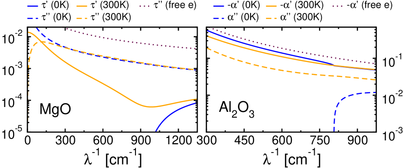
Figure 1: Dimensionless surface conductivity $\tau=\tau^{\prime}+i\tau^{\prime\prime}$ for MgO for $n_{s}=10^{13}cm^{-2}$ (left) and polarizability of excess electrons $\alpha=\alpha^{\prime}+i\alpha^{\prime\prime}$ for Al₂O₃ for $n_{b}=3\times 10^{17}cm^{-3}$ (right) as a function of the inverse wavelength $\lambda^{-1}$.

For $\chi>0$ the bulk conductivity is limited by a longitudinal optical (LO) phonon with frequency $\omega_{LO}$. The coupling of the electron to this mode is described by $H_{int}=\sum_{\mathbf{k},\mathbf{q}}Mc_{\mathbf{k}+\mathbf{q}}^{\dagger}c_{\mathbf{k}}\left(a_{\mathbf{q}}+a_{-\mathbf{q}}^{\dagger}\right)/\sqrt{V}q$ Mahan (1990), where $M=\sqrt{2\pi e^{2}\hbar\omega_{LO}\left(\epsilon_{\infty}^{-1}-\epsilon_{0}^{-1}\right)}$. Employing the memory function approach, the bulk conductivity is given by Eq. (3) where $n_{s}$ is replaced by the bulk electron density $n_{b}$ and $m$ by the conduction band effective mass $m^{\ast}$, the prefactor of the memory function (Eq. (4)) is then $4e^{2}\sqrt{m^{\ast}\omega_{LO}\delta}(\epsilon_{\infty}^{-1}-\epsilon_{0}^{-1})/(3\sqrt{(2\pi\hbar)^{3}})$, and

$$j(\nu)= \frac{e^{\delta}}{e^{\delta}-1}|\nu+1|e^{-\delta(\nu+1)/2}K_{1}\left(\delta|\nu+1|/2\right)$$

$$+ \frac{1}{e^{\delta}-1}|\nu-1|e^{-\delta(\nu-1)/2}K_{1}\left(\delta|\nu-1|/2\right)\text{ ,}$$ (6)

where $\nu=\omega/\omega_{LO}$, $\delta=\beta\hbar\omega_{LO}$, and $K_{1}(x)$ is a modified Bessel function. For low temperature, i.e. $\delta\rightarrow\infty$ $j(\nu)\sim\sqrt{\pi/\delta}\sqrt{|\nu+1|}\theta(-\nu-1)$.

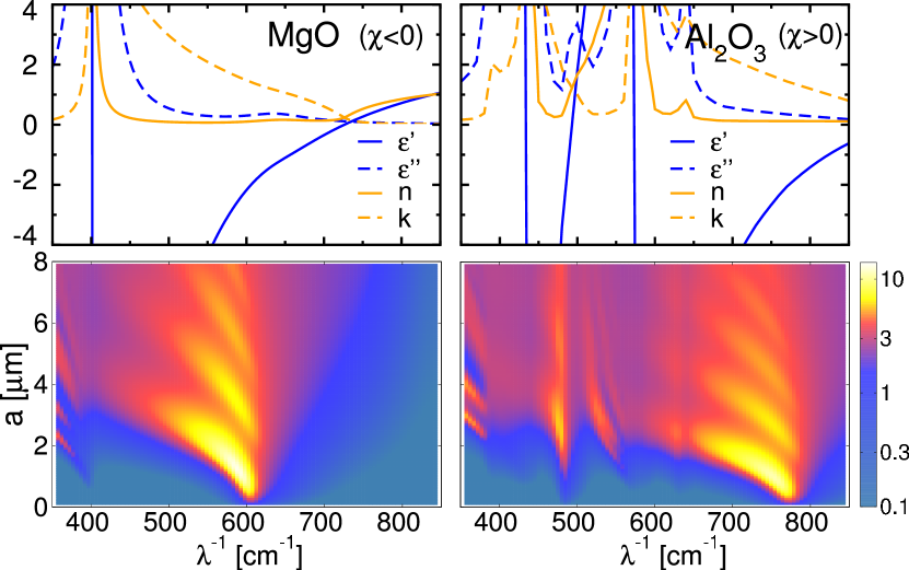
Figure 2: Dielectric constant $\epsilon=\epsilon^{\prime}+i\epsilon^{\prime\prime}$, refractive index $N=n+ik$ (top) and extinction efficiency $Q_{t}$ (bottom) depending on the particle radius $a$ for MgO and Al₂O₃ as a function of the inverse wavelength $\lambda^{-1}$.

To exemplify light scattering by a charged dielectric particle we will consider a MgO ($\chi<0$) and an Al₂O₃ ($\chi>0$) particle mat . The charge effect on scattering is controlled by the dimensionless surface conductivity $\tau=\tau^{\prime}+i\tau^{\prime\prime}$ (for $\chi<0$) or the excess electron polarizability $\alpha=\alpha^{\prime}+i\alpha^{\prime\prime}$ (for $\chi>0$), both shown in Fig. 1, which are small even for a highly charged particle with $n_{s}=10^{13}cm^{-2}$ (corresponding to $n_{b}=3\times 10^{17}cm^{-3}$ for $\chi>0$ and $a=1\mu m$). The electron-phonon coupling reduces $\tau^{\prime\prime}$ and $\alpha^{\prime}$ compared to a free electron gas where $M(\omega)=0$, implying $\tau^{\prime}=0$ and $\alpha^{\prime\prime}=0$. For $T=0K$, $\tau^{\prime}=0$ ($\alpha^{\prime\prime}=0$) for $\lambda^{-1}<\lambda_{s}^{-1}=909cm^{-1}$, the inverse wavelength of the surface phonon ( $\lambda^{-1}<\lambda_{LO}^{-1}=807cm^{-1}$, the inverse wavelength of the bulk LO phonon) since light absorption is only possible above the surface (bulk LO) phonon frequency. At room temperature $\tau^{\prime\prime}$ and $\alpha^{\prime}$ still outweigh $\tau^{\prime}$ and $\alpha^{\prime\prime}$. The temperature effect on $\tau^{\prime\prime}$ is less apparent for $\lambda^{-1}>300cm^{-1}$ than for $\alpha^{\prime}$ but for $\lambda^{-1}<300cm^{-1}$ a higher temperature lowers $\tau^{\prime\prime}$ considerably. The upper panel of Fig. 2 shows the complex dielectric constant $\epsilon$ and the refractive index $N$. For MgO we use a two-oscillator fit for $\epsilon$ Jasperse et al. (1966); Palik (1985). In the infrared, $\epsilon$ is dominated by a TO phonon at $401cm^{-1}$. The second phonon at $640cm^{-1}$ is much weaker, justifying our model for the image potential based on one dominant phonon. Far above the highest TO phonon, that is, for $\lambda^{-1}>800cm^{-1}$ ($\lambda^{-1}>900cm^{-1}$) for MgO (Al₂O₃) $\epsilon^{\prime}>0$ and $\epsilon^{\prime\prime}\ll 1$. For these wavenumbers a micron sized grain would give rise to a typical Mie plot exhibiting interference and ripples due to the functional form of $a_{n}^{r}$ and $b_{n}^{r}$ and not due to the dielectric constant. Surplus electrons would not alter the extinction in this region because $|\epsilon|\gg|\tau|$ and $|\epsilon|\gg|\alpha|$.

To observe a stronger dependence of extinction on the parameters $\epsilon$ and $\tau$ or $\alpha$, we turn to $400cm^{-1}<\lambda^{-1}<700cm^{-1}$ for MgO ($700cm^{-1}<\lambda^{-1}<900cm^{-1}$ for Al₂O₃) where $\epsilon^{\prime}<0$ and $\epsilon^{\prime\prime}\ll 1$ allowing for optical resonances, sensitive to even small changes in $\epsilon$. They correspond to resonant excitation of transverse surface modes of the sphere Fuchs and Kliewer (1968). For a metal particle the resonances are due to plasmons and lie in the ultraviolet Tribelsky and Lykyanchuk (2006); Tribelsky (2011). For a dielectric the TO phonon induces them. As the polarizability of excess electrons, encoded in $\tau$ or $\alpha$, is larger at low frequency, the resonances of a dielectric particle, lying in the infrared, should be more susceptible to surface charges. The lower panel of Fig. 2 shows a clearly distinguishable series of resonances in the extinction efficiency. The effect of negative excess charges is shown by the crosses in Fig. 3. The extinction maxima are shifted to higher $\lambda^{-1}$ for both surface and bulk excess electrons. For comparison the circles show the shift for a free electron gas. The effect is strongest for the first resonance, where a surface electron density $10^{13}cm^{-2}$ (or an equivalent bulk charge), realized for instance in dusty plasmas Fortov et al. (2011), yields a shift of a few wavenumbers.

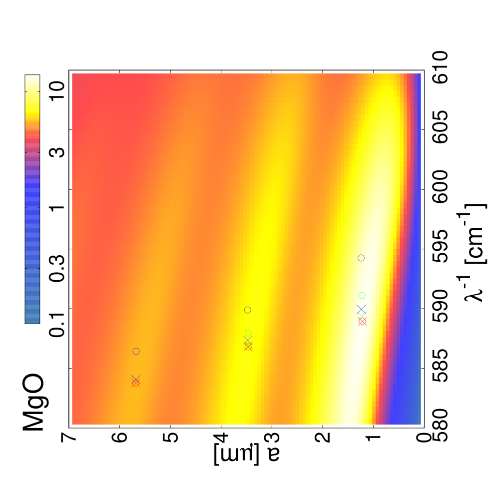
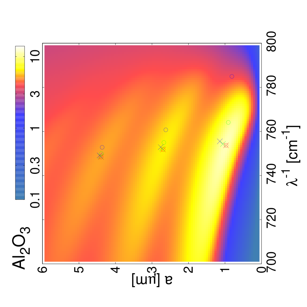
Figure 3: Magnification of the extinction resonances depending on $\lambda^{-1}$ and $a$. Crosses indicate their maxima for $n_{s}=0$ (red), $2\times 10^{13}$ (green), and $5\times 10^{13}cm^{-2}$ (blue) at $T=300K$ for MgO (left panel) and for $n_{b}=3n_{s}/a$ for Al₂O₃ (right panel). Open circles indicate the maxima for free electrons.

The shift can be more clearly seen in Fig. 4 where the tail of the first resonance is plotted for MgO on an enlarged scale. The main panel shows the extinction efficiency for $n_{s}=10^{13}cm^{-2}$ with its maxima indicated by blue dots. Without surface charge the resonance is at $\lambda^{-1}=606cm^{-1}$ for $a<0.25\mu m$. For a charged particle it moves to higher $\lambda^{-1}$ and this effect becomes stronger the smaller the particle is. The line shape of the extinction resonance for fixed particle size is shown in the top and bottom panels for $a=0.2\mu m$ and $a=0.05\mu m$, respectively. For comparison data for other surface charge densities are also shown. Figure 4 also suggests that the resonance shift is even more significant for particles with radius $a<0.01\mu m$ where the planar model for the image states is inapplicable. An extension of our model, guided by the study of multielectron bubbles in helium Tempere et al. (2007), requires surface phonons, image potential and electron-phonon coupling for a sphere. Due to its insensitivity to the location of the excess electrons, we expect qualitatively the same resonance shift for very small grains.

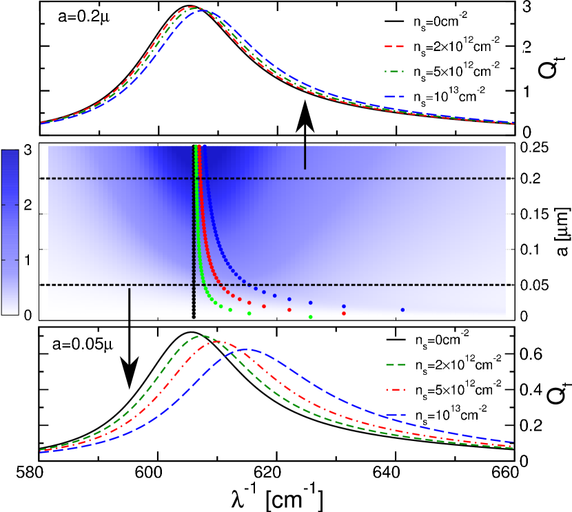
Figure 4: Middle panel: Extinction efficiency $Q_{t}$ as a function of the inverse wavelength $\lambda^{-1}$ and the radius $a$ for a MgO particle with $n_{s}=10^{13}cm^{-2}$ and $T=300K$. The dotted lines indicate the extinction maximum for $n_{s}=0$ (black), $2\times 10^{12}$ (green), $5\times 10^{12}$ (red), and $10^{13}cm^{-2}$ (blue) obtained from (8). Top and bottom panel: Extinction efficiency $Q_{t}$ as a function of $\lambda^{-1}$ for $a=0.2\mu m$ (top) and $a=0.05\mu m$ (bottom) for different surface electron densities.

As we are considering particles small compared to $\lambda$ we expand the scattering coefficients for small $\rho$. To ensure that in the limit of an uncharged grain, that is, for $\tau\rightarrow 0$, $a_{n}^{r}$ and $b_{n}^{r}$ converge to their small $\rho$ expansions Stratton (1941), we substitute $t=\tau/\rho$ before expanding the coefficients. Up to $\mathcal{O}(\rho^{3})$ this yields $a_{1}^{r}=a_{2}^{r}=b_{2}^{r}=0$ and only $b_{1}^{r}\sim\mathcal{O}(\rho^{3})$ contributes. Then the extinction efficiency,

$$Q_{t}=\frac{12\rho\left(\epsilon^{\prime\prime}+\alpha^{\prime\prime}+2\tau^{\prime}/\rho\right)}{\left(\epsilon^{\prime}+\alpha^{\prime}+2-2\tau^{\prime\prime}/\rho\right)^{2}+\left(\epsilon^{\prime\prime}+\alpha^{\prime\prime}+2\tau^{\prime}/\rho\right)^{2}}~{},$$ (7)

where the excess charges enter either through $\tau$ with $\alpha=0$ for $\chi<0$ or through $\alpha$ with $\tau=0$ for $\chi>0$. For $\tau,\alpha\rightarrow 0$ this gives the limit of Rayleigh scattering. The resonance is located at the wavenumber where

$$\epsilon^{\prime}+\alpha^{\prime}+2-2\tau^{\prime\prime}/\rho=0\text{ }$$ (8)

and has a Lorentzian shape, already apparent from Fig. 4, provided $\epsilon^{\prime\prime}$ and $\tau^{\prime}$ (or $\alpha^{\prime\prime}$) vary only negligibly near the resonance wavelength. For an uncharged surface the resonance is at $\lambda_{0}^{-1}$ for which $\epsilon^{\prime}=-2$. For $\chi<0$ the shift of the resonance is proportional to $\tau^{\prime\prime}$ and thus to $n_{s}$, provided $\epsilon^{\prime}$ is well approximated linearly in $\lambda^{-1}$ and $\tau^{\prime\prime}$ does not vary significantly near $\lambda_{0}^{-1}$. In this case, we substitute in (8) the expansions $\epsilon^{\prime}=-2+c_{\epsilon}(\lambda^{-1}-\lambda_{0}^{-1})$ and $\tau^{\prime\prime}=c_{\tau}n_{s}$ where $c_{\epsilon}=\frac{\partial\epsilon^{\prime}}{\partial\lambda^{-1}}|_{\lambda_{0}^{-1}}$ and $c_{\tau}=\frac{\tau^{\prime\prime}}{n_{s}}|_{\lambda_{0}^{-1}}$. Then the resonance is located at $\lambda^{-1}=\lambda_{0}^{-1}+c_{\tau}n_{s}/(\pi c_{\epsilon}a\lambda_{0}^{-1})$. For $\chi>0$ the resonance is located at $\lambda^{-1}=\lambda_{0}^{-1}-c_{\alpha}n_{b}/c_{\epsilon}$ where $c_{\alpha}=\frac{\alpha^{\prime}}{n_{b}}|_{\lambda_{0}^{-1}}$. The dotted lines in Fig. 4 give the location of the resonance obtained from Eq. (8) for MgO, where $\lambda_{0}^{-1}=606cm^{-1}$ for several surface electron densities. They agree well with the underlying contour calculated from the exact Mie solution, as exemplified for $n_{s}=10^{13}cm^{-2}$. The proportionality of the resonance shift to $n_{s}$ ($n_{b}$) can also be seen in Fig. 5 where we plot on the abscissa the shift of the extinction resonance arising from the surface electron density given on the ordinate for LiF mat , MgO ($\chi<0$) and Al₂O₃ ($\chi>0$). Both bulk and surface electrons lead to a resonance shift. To illustrate the similarity of the shift we consider (8) for free electrons, which then becomes $\epsilon^{\prime}-2N_{e}e^{2}/(ma^{3}\omega^{2})=-2$ for $\chi<0$ and $\epsilon^{\prime}-3N_{e}e^{2}/(m^{\ast}a^{3}\omega^{2})=-2$ for $\chi>0$; $N_{e}$ is the number of excess electrons. The effect of surface electrons is weaker by a factor $2m^{\ast}/3m$ where the $2/3$ arises from geometry as only the parallel component of the electric field acts on the spherically confined electrons. Most important, however, $\tau/\rho$ and $\alpha$ enter the resonance condition on the same footing showing that the shift is essentially an electron density effect on the polarizability of the grain. We therefore expect the shift to prevail also for electron distributions between the two limiting cases of a surface and a homogeneous bulk charge.

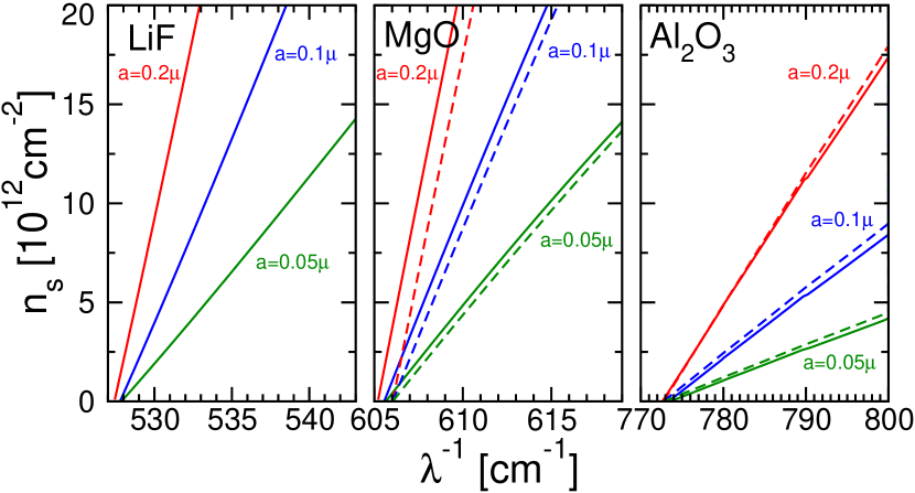
Figure 5: Position of the extinction resonance depending on the surface charge $n_{s}$ for LiF , MgO and Al₂O₃ (for equivalent bulk charge $n_{b}=3n_{s}/a$) particles with different radii $a$. Solid (dashed) lines are obtained from the Mie contour (Eq. (8)).

To conclude, our results suggest that for dielectric particles showing anomalous optical resonances the extinction maximum in the infrared can be used to determine the particle charge (see Fig. 5). For dusty plasmas this can be rather attractive because established methods for measuring the particle charge Carstensen et al. (2011); Khrapak et al. (2005); Tomme et al. (2000) require plasma parameters which are not precisely known whereas the charge measurement by Mie scattering does not. Particles with surface (negative electron affinity $\chi$, e.g. MgO, LiF) as well as bulk excess electrons ($\chi>0$ e.g. Al₂O₃) show the effect and could serve as model systems for sub-micron sized dust in space, the laboratory, and the atmosphere. These particles could be also used as minimally invasive electric probes in a plasma, which collect electrons depending on the local plasma environment. Determining their charge from Mie scattering and the forces acting on them by conventional means Carstensen et al. (2011); Khrapak et al. (2005); Tomme et al. (2000) would provide a way to extract plasma parameters locally.

We acknowledge support by the Deutsche Forschungsgemeinschaft through SFB-TRR 24, Project B10.

References

- Mie (1908) G. Mie, Ann. Phys. (Leipzig) 25, 377 (1908).
- Bohren and Huffman (1983) C. F. Bohren and D. R. Huffman, Absorption and Scattering of Light by small particles (Wiley, 1983).
- Born and Wolf (1999) M. Born and E. Wolf, Principles of Optics (Cambridge University Press, 1999).
- Heifetz et al. (2010) A. Heifetz, H. T. Chien, S. Liao, N. Gopalsami, and A. C. Raptis, J. of Quantitative Spectroscopy and Radiative Transfer 111, 2550 (2010).
- Friedrich and Rapp (2009) M. Friedrich and M. Rapp, Surv. Geophys. 30, 525 (2009).
- Mann (2008) I. Mann, Advances in Space Research 41, 160 (2008).
- Ishihara (2007) O. Ishihara, J. Phys. D: Appl. Phys 40, R121 (2007).
- Mendis (2002) D. A. Mendis, Plasma Sources Sci. Technol. 11, A219 (2002).
- Klačka and Kocifaj (2010) J. Klačka and M. Kocifaj, Progress in Electromagnetics Research 109, 17 (2010).
- Klačka and Kocifaj (2007) J. Klačka and M. Kocifaj, J. of Quantitative Spectroscopy and Radiative Transfer 106, 170 (2007).
- Bohren and Hunt (1977) C. F. Bohren and A. J. Hunt, Can. J. Phys. 55, 1930 (1977).
- Rohlfing et al. (2003) M. Rohlfing, N.-P. Wang, P. Kruger, and J. Pollmann, Phys. Rev. Lett. 91, 256802 (2003).
- Baumeier et al. (2007) B. Baumeier, P. Kruger, and J. Pollmann, Phys. Rev. B 76, 205404 (2007).
- Heinisch et al. (2011) R. L. Heinisch, F. X. Bronold, and H. Fehske, Phys. Rev. B 83, 195407 (2011).
- Heinisch et al. (2012) R. L. Heinisch, F. X. Bronold, and H. Fehske, Phys. Rev. B 85, 075323 (2012).
- Tribelsky and Lykyanchuk (2006) M. I. Tribelsky and B. S. Lykyanchuk, Phys. Rev. Lett. 97, 263902 (2006).
- Tribelsky (2011) M. I. Tribelsky, Europhys. Lett. 94, 14004 (2011).
- Stratton (1941) J. A. Stratton, Electromagnetic theory (McGraw-Hill, 1941).
- Evans and Mills (1973) E. Evans and D. L. Mills, Phys. Rev. B 8, 4004 (1973).
- Barton (1981) G. Barton, J. Phys. C 14, 3975 (1981).
- Kato and Ishii (1995) M. Kato and A. Ishii, Appl. Surf. Sci. 85, 69 (1995).
- Götze and Wölfle (1972) W. Götze and P. Wölfle, Phys. Rev. B 6, 1226 (1972).
- Mahan (1990) G. D. Mahan, Many-particle physics (Plenum, 1990), p. 703-708.
- (24) We use for MgO Wintersgill et al. (1979), and from Jasperse et al. (1966), for LiF Dolling et al. (1968), Dolling et al. (1968) and from Hofmeister et al. (2003), and for Al2O3 , , Schubert et al. (2000), Perevalov et al. (1979) and from Palik (1985).
- Jasperse et al. (1966) J. R. Jasperse, A. Kahan, J. N. Plendl, and S. S. Mitra, Phys. Rev. 146, 526 (1966).
- Palik (1985) E. D. Palik, Handbook of Optical Constants of Solids (Academic, 1985).
- Fuchs and Kliewer (1968) R. Fuchs and K. L. Kliewer, J. Opt. Soc. Am. 58, 319 (1968).
- Fortov et al. (2011) V. E. Fortov, A. V. Gavrikov, O. F. Petrov, V. S. Sidorov, M. N. Vasiliev, and N. A. Vorona, Europhys. Lett. 94, 55001 (2011).
- Tempere et al. (2007) J. Tempere, I. Silvera, and J. Devreese, Surf. Sci. Rep. 62, 159 (2007).
- Carstensen et al. (2011) J. Carstensen, H. Jung, F. Greiner, and A. Piel, Phys. Plasmas 18, 033701 (2011).
- Khrapak et al. (2005) S. A. Khrapak, S. V. Ratynskaia, A. V. Zobnin, A. D. Usachev, V. V. Yaroshenko, M. H. Thoma, M. Kretschmer, H. Hoefner, G. E. Morfill, O. F. Petrov, et al., Phys. Rev. E 72, 016406 (2005).
- Tomme et al. (2000) E. B. Tomme, D. A. Law, B. M. Annaratone, and J. E. Allen, Phys. Rev. Lett. 85, 2518 (2000).
- Wintersgill et al. (1979) M. Wintersgill, J. Fontanella, C. Andeen, and D. Schuele, J. Appl. Phys. 50, 8259 (1979).
- Dolling et al. (1968) G. Dolling, H. G. Smith, R. M. Nicklow, P. R. Vijayaraghavan†, and M. K. Wilkinson, Phys. Rev. 168, 970 (1968).
- Hofmeister et al. (2003) A. M. Hofmeister, E. Keppel, and A. K. Speck, Mon. Not. R. Astron. Soc. 345, 16 (2003).
- Schubert et al. (2000) M. Schubert, T. E. Tiwald, and C. M. Herzinger, Phys. Rev. B 61, 8187 (2000).
- Perevalov et al. (1979) T. V. Perevalov, A. V. Shaposhnikov, V. A. Gritsenko, H. Wong, and J. H. H. und C. W. Kim, JETP Letters 85, 165 (1979).