Einstein relation in superdiffusive systems

Abstract

We study the Einstein relation between diffusion and response to an external field in systems showing superdiffusion. In particular, we investigate a continuous time Lévy walk where the velocity remains constant for a time $\tau$ with distribution $P_{\tau}(\tau)\sim\tau^{-g}$. At varying $g$ the diffusion can be standard or anomalous; in spite of this, if in the unperturbed system a current is absent, the Einstein relation holds. In the case where a current is present the scenario is more complicated and the usual Einstein relation fails. This suggests that the main ingredient for the breaking of the Einstein relation is not the anomalous diffusion but the presence of a mean drift (current).

1 Introduction

The fluctuation-dissipation relation (FDR) is one of the fundamental results of the statistical physics [1]. In his celebrated work on the Brownian motion, Einstein gave the first example of FDR. In the absence of external forcing, at large times, one has

$$\langle x(t)\rangle=0\qquad\textrm{and}\qquad\langle x^{2}(t)\rangle\simeq 2Dt,$$ (1)

where $x$ is the position of the colloidal particle, $D$ is the diffusion coefficient and the average refers to the unperturbed dynamics. If a small constant external force $\mathcal{E}$ is applied, one obtains a linear drift

$$\langle x(t)\rangle_{\mathcal{E}}\simeq\mu\mathcal{E}t,$$ (2)

where $\langle\ldots\rangle_{\mathcal{E}}$ is the average on the perturbed system, and $\mu$ is the mobility. The remarkable result obtained by Einstein is the proportionality between $\langle x(t)\rangle_{\mathcal{E}}$ and the mean square displacement (MSD) $\langle x^{2}(t)\rangle$:

$${\langle x^{2}(t)\rangle\over\langle x(t)\rangle_{\mathcal{E}}}=\frac{2}{\beta\mathcal{E}},$$ (3)

namely $\mu=\beta D$, where $\beta$ is the inverse temperature and we have taken the Boltzmann constant $k_{B}=1$.

In the last decades many researches have been devoted to the study of anomalous diffusion, where, instead of (1), one has

$$\langle x^{2}(t)\rangle\sim t^{2\nu}\qquad\mbox{with}\qquad\nu\neq 1/2,$$ (4)

see for instance [2, 3, 4, 5, 6, 7]. The case $\nu<1/2$ is called subdiffusion while if $\nu>1/2$ we are in the presence of superdiffusion. It is quite natural to wonder about the validity of the FDR in these anomalous situations. Important results showing the proportionality between $\langle x(t)\rangle_{\mathcal{E}}$ and $\langle x^{2}(t)\rangle$, which we refer to as the Einstein relation “at equilibrium”, have already been obtained for both superdiffusive [8, 9, 7] and subdiffusive [2, 10, 7] anomalous dynamics. Differently, the situation where the drift is compared to the mean square displacement in a state which is already “out of equilibrium”, either due to a current [11] or due to dissipation [12], has been studied only in the subdiffusive cases.

The aim of this letter is to discuss the validity of the Einstein relation in equilibrium and out-of-equilibrium situations in the presence of superdiffusive dynamics. In particular, we consider a Lévy walk collision process [13] and we show that the Einstein relation is violated when the perturbation is applied on a reference state where a current is already present.

2 The model

We consider an ensemble of probe particles of mass $m$ endowed with scalar velocity $v$ and position $x$. Each probe particle only interacts with particles of mass $M$ and velocity $V$ extracted from an equilibrium bath at temperature $T$. We assume that the scattering probability does not depend on the relative velocity between the probe particle and the colliders, as, for instance, in the case of Maxwell-molecule models [14]. Velocity of the probe particle changes from $v$ to $v^{\prime}$ at each collision, according to the rule:

$$v^{\prime}=\gamma v+(1-\gamma)V,$$ (5)

where $\gamma=(\zeta-\alpha)/(1+\zeta)$, with $\zeta=m/M$, and $\alpha$ is the coefficient of restitution ($\alpha=1$ for an elastic collision). The velocity $V$ of the bath particles is a random variable generated from a Gaussian distribution with zero mean and variance $T/M$:

$$P_{S}(V)=\sqrt{\frac{M}{2\pi T}}\exp\left\{-\frac{M}{2T}V^{2}\right\}.\\$$ (6)

The elementary step of the dynamics is made by: i) a flight, $x(t+\tau)=x(t)+v^{\prime}\tau+1/2\mathcal{E}\tau^{2}$, where $x(t)$ is the position of the probe particle at time $t$, with $\tau$ taken from a distribution $P_{\tau}(\tau)$ and $\mathcal{E}$ a constant acceleration, followed by ii) a collision $v^{\prime}=\gamma v+(1-\gamma)V$, with $V$ taken from the Gaussian distribution (6). In the specific case $\alpha=1$ and $M=m$, one has $\gamma=0$ and the collision rule (5) results in a random update of the velocity according to the distribution (6). The duration of each flight, $\tau$, is an independent identically distributed random variable with probability

$$P_{\tau}(\tau)\sim\tau^{-g},$$ (7)

with $g>1$. This kind of process is called Lévy walk collision process [13], and may be interpreted as due to scattering centers randomly distributed on a fractal spatial structure, as for instance in the case of molecular diffusion in porous media [15]. If $\alpha\neq 1$ or $m\neq M$, with $\alpha\neq\zeta$, a dependence on the last velocity before the collision remains. In this case velocity correlations can be measured in the system, as discussed in Section 3.1.

According to the dynamic rules of the process described above the displacement of the probe particle is always finite in a finite time. The anomalous dynamics of such a model has been studied in [16], showing that the process is an example of “strong” anomalous diffusion, namely that it is not possible to find a scaling for the probability density function (PDF) of displacements. Such a collision process becomes a standard diffusive system when $P_{\tau}$ decays fast enough: in this regime the dynamics is qualitatively equivalent to that of a system with exponential $P_{\tau}$, studied for instance in [17, 18, 19]. Lévy walk collision processes have been thoroughly studied, see for instance [7], where the behavior of the mean square displacement has been obtained analytically.

We recall here a simple argument already presented in [16] to study the asymptotic behavior of higher order moments of displacement, and that can be easily applied also to the case with an external perturbing field that we are going to discuss here in Section 3. In order to obtain in a simple way the dominant asymptotic behavior of $\langle x^{2}(t)\rangle$, we introduce a cut-off $t_{c}$ for $P_{\tau}(\tau)$:

$$P_{\tau}(\tau)\sim\left\{\begin{array}[]{ll}\tau^{-g}&\textrm{if $\tau<t_{c}$}\\ 0&\textrm{if $\tau>t_{c}$.}\\ \end{array}\right.$$ (8)

Assuming $x=0$ as initial condition for each trajectory, the mean square displacement after the time $t$, where $N(t)$ collisions occurred, can be written in full generality as:

$$\langle x^{2}(t)\rangle=\left\langle\left[\sum_{i=1}^{N(t)}v_{i}\tau_{i}\right]^{2}\right\rangle\simeq\sum_{i=1}^{\overline{N}(t)}\left\langle v^{2}_{i}\tau^{2}_{i}\right\rangle+2\overline{N}(t)\sum_{i=1}^{\overline{N}(t)}\left\langle v_{i}v_{0}\tau_{i}\tau_{0}\right\rangle.$$ (9)

Here, $v_{i}$ denotes the velocity of the probe particle after the $i$-th collision, $\tau_{i}$ is the time elapsed between the collisions $i$ and $i+1$ and $\overline{N}(t)$ is the average number of collisions occurred up to time $t$. The average $\langle\cdots\rangle$ is taken over the distributions (6) and (7). From Eq. (8) we have, for $n+1-g>0$,

$$\langle\tau^{n}\rangle_{c}\sim t_{c}^{n+1-g},$$ (10)

where $\langle\cdots\rangle_{c}$ denotes an average over the distribution (8) with the cut-off $t_{c}$.

We start by considering the case with independent velocities $v_{i}$, corresponding to a choice of parameters such that $\gamma=0$. Then, estimating $\langle x^{2}(t)\rangle$ at a time $t\gg t_{c}$, so that the average number of collisions along the trajectory can be approximated to $\overline{N}(t)\simeq t/\langle\tau\rangle_{c}$, and considering that the cross terms in Eq. (9) are zero, we can write

$$\langle x^{2}(t)\rangle\simeq\frac{t}{\langle\tau\rangle_{c}}\langle v^{2}\rangle\langle\tau^{2}\rangle_{c}.$$ (11)

In the case $g>3$, both $\langle\tau\rangle_{c}$ and $\langle\tau^{2}\rangle_{c}$ are finite, even in the limit $t_{c}\rightarrow\infty$, so that we find the simple diffusive behavior $\langle x^{2}(t)\rangle\sim t$. For $t\lesssim t_{c}$ and $1<g<3$, instead of (11) we expect

$$\langle x^{2}(t)\rangle\sim t^{2\nu}.$$ (12)

One can easily find the exponent $\nu$ with a matching argument. Comparing (11) and (12) at $t\sim t_{c}$ and using (10), we obtain $\nu=1/2$ for $g>3$, $\nu=2-g/2$ for $2<g<3$, and $\nu=1$ for $1<g<2$ (logarithmic corrections appear at the values $g=2$ and $g=3$ [7]).

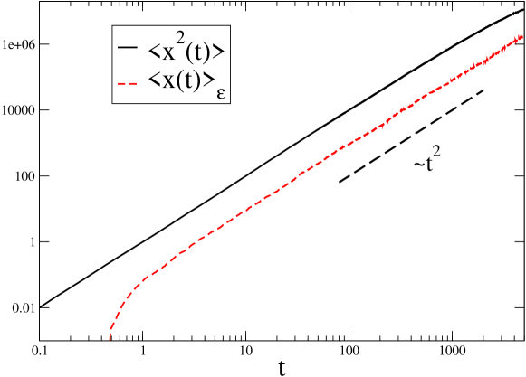
Figure 1: Log-Log plot of the MSD in the case of superdiffusive dynamics with $g=3/2$, $\langle x^{2}(t)\rangle$ (black line), and of the drift $\langle x(t)\rangle_{\mathcal{E}}$ (red dashed line) in the case of uniform external field $\mathcal{E}=1.5$. Both quantities behave as $\sim t^{2}$ and the Einstein relation is verified.

3 Einstein relation

The main concern of our study is the question about the validity of the Einstein relation for superdiffusive anomalous dynamics. In particular such a relation can be checked in two different situations:

(A)

The drift due to the external force is compared with the MSD of the probe particle in the absence of any pulling force. This case corresponds to a fluctuation-dissipation experiment realized by switching on from zero the external perturbation.

(B)

The drift is compared to the MSD in a state where a current is already present. This procedure corresponds to increase the intensity of the perturbation in a state already perturbed and compare the average current in this state with the fluctuations in the initial reference state.

In the following, we will refer to situation (A) as a test of the fluctuation-dissipation relation at equilibrium while to case (B) as a test out of equilibrium. We will show that these two cases are very different.

3.1 Perturbation of a state without current

The argument used in Sec. 2 to study the MSD can be applied to the drift, yielding

$$\langle x(t)\rangle_{\mathcal{E}}=\langle\sum_{i=1}^{N(t)}\left(v_{i}\tau_{i}+\frac{\mathcal{E}}{2}\tau_{i}^{2}\right)\rangle=\frac{t}{\langle\tau\rangle_{c}}\left[\langle\tau\rangle_{c}\langle v\rangle+\frac{\mathcal{E}}{2}\langle\tau^{2}\rangle_{c}\right]=\frac{\mathcal{E}}{2}\frac{t}{\langle\tau\rangle_{c}}\langle\tau^{2}\rangle_{c},$$ (13)

which perfectly matches the result for the MSD found in Eq. (11). Therefore, when we perturb an equilibrium state, namely a state without currents, we have for any value of $g>1$

$$\frac{\langle x^{2}(t)\rangle}{\langle x(t)\rangle_{\mathcal{E}}}=\textrm{const}.$$ (14)

Let us note that the Einstein relation holds quite generally, namely it persists even if we make our process non-Markovian by allowing some memory across collisions, that is, we put $\gamma>0$ in the collision rule Eq. (5), preventing a complete reshuffling of velocities. In this case the MSD reads as:

$$\langle x^{2}(t)\rangle=\sum_{i,j}^{\overline{N}(t)}\langle v_{i}\tau_{i}v_{j}\tau_{j}\rangle\sim\frac{t}{\langle\tau\rangle_{c}}\left[\langle v^{2}\rangle\langle\tau^{2}\rangle_{c}+2\langle\tau\rangle_{c}^{2}\sum_{i}^{\overline{N}(t)}\langle v_{i}v_{0}\rangle\right],$$ (15)

because the collision times are still not dependent on the velocity but correlations between the velocities must be taken into account. Note that, even in the presence of non-independent $\{v_{i}\}$, if $\sum_{i}^{n}\langle v_{i}v_{0}\rangle$ yields a finite contribution at large times the second term on the right of Eq. (15) grows as $\langle\tau\rangle_{c}^{2}$, namely it is subdominant compared to $\langle\tau^{2}\rangle_{c}$ in all situations. If the exponent of the flight time distribution is $1<g<2$, then $\langle\tau^{2}\rangle_{c}\sim t^{3-g}>t^{4-2g}\sim\langle\tau\rangle_{c}^{2}$; if $2<g<3$ we have that $\langle\tau\rangle_{c}^{2}$ is a finite number, while for $g>3$ we recover a simple diffusive behavior for both the MSD and the drift. In particular, in the case $g>3$ the presence of correlations of velocities amounts to a renormalization of the diffusion coefficient.

We conclude that the asymptotic behavior of the MSD is the same as in Eq. (11). From Eq. (13) one can see that no cross correlations between velocities at different times appear, so that the drift is not influenced by velocities correlations across collisions. Therefore, we can conclude that the Einstein relation is preserved for all values of the exponent $g$ of the flight times distribution. This example shows how the Einstein relation is a stable result, valid under quite general conditions also in the presence of anomalous dynamics [7, 20, 11].

3.2 Perturbation of a state with a current

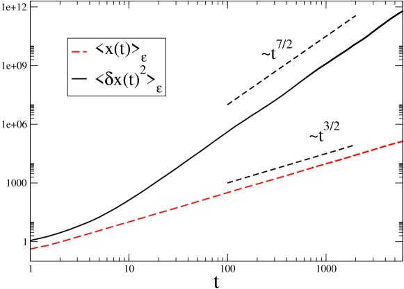
Figure 2: Log-Log plot of the MSD (black line) in the presence of a constant external field $\mathcal{E}=1.5$ and drift (red dashed line) with the same value of the field, in the case of superdiffusive dynamics with $g=5/2$. We observe a breaking of the Einstein relation with leading asymptotic behaviors, $\langle[\delta x(t)]^{2}\rangle_{\mathcal{E}}\sim t^{7/2}$, see Eq. (18), and $\langle x(t)\rangle_{\mathcal{E}}\sim t^{3/2}$, see Eq. (13).

In order to study the Einstein relation out of equilibrium, let us first consider a simple Gaussian process, namely the Brownian motion of a colloidal particle when we add a constant force pulling the particle. In this case it is sufficient to replace the MSD around the average position $\langle[\delta x(t)]^{2}\rangle_{\mathcal{E}}=\langle x^{2}(t)\rangle_{\mathcal{E}}-\langle x(t)\rangle^{2}_{\mathcal{E}}$ for the simple MSD, in order to recover the Einstein relation with the drift $\langle x(t)\rangle_{\mathcal{E}+\delta\mathcal{E}}-\langle x(t)\rangle_{\mathcal{E}}$ (here $\langle\cdots\rangle_{\mathcal{E}+\delta\mathcal{E}}$ denotes the average over a state where the further perturbation $\delta\mathcal{E}$ is applied). In what follows we consider that a non trivial violation of the Einstein relation happens when also the MSD around the drift lacks the proportionality with the drift itself. This is indeed the case of superdiffusive dynamics.

For simplicity we will refer to the case $\gamma=0$ but the physical picture remains the same also when the case with memory is considered. In our model, by applying the constant field $\mathcal{E}>0$, we have:

$$\langle x^{2}(t)\rangle_{\mathcal{E}} = \langle\left[\sum_{i=1}^{N(t)}\left(v_{i}\tau_{i}+\frac{\mathcal{E}}{2}\tau_{i}^{2}\right)\right]^{2}\rangle_{t_{c}}$$ (16)

$$\simeq \frac{\mathcal{E}^{2}}{4}t^{2}\frac{\langle\tau^{2}\rangle_{c}^{2}}{\langle\tau\rangle_{c}^{2}}+t\left(\frac{\mathcal{E}^{2}}{4}\frac{\langle\tau^{4}\rangle_{c}-\langle\tau^{2}\rangle^{2}_{c}}{\langle\tau\rangle_{c}}+\frac{\langle v^{2}\rangle\langle\tau^{2}\rangle_{c}}{\langle\tau\rangle_{c}}\right)$$

$$\langle[\delta x(t)]^{2}\rangle_{\mathcal{E}} = \langle x^{2}(t)\rangle_{\mathcal{E}}-\langle x(t)\rangle^{2}_{\mathcal{E}}\simeq t\left(\frac{\mathcal{E}^{2}}{4}\frac{\langle\tau^{4}\rangle_{c}-\langle\tau^{2}\rangle^{2}_{c}}{\langle\tau\rangle_{c}}+\frac{\langle v^{2}\rangle\langle\tau^{2}\rangle_{c}}{\langle\tau\rangle_{c}}\right).$$ (17)

In the case $2<g<3$, namely when the the distribution $P_{\tau}(\tau)$ has finite mean and infinite variance, the diffusion around the average position behaves asymptotically as

$$\langle[\delta x(t)]^{2}\rangle_{\mathcal{E}}\simeq t\left(\frac{\mathcal{E}^{2}}{4}\frac{t_{c}^{5-g}-t_{c}^{6-2g}}{\langle\tau\rangle_{c}}+\frac{\langle v^{2}\rangle t_{c}^{3-g}}{\langle\tau\rangle_{c}}\right).$$ (18)

Considering for instance the case $g=5/2$, by applying the matching argument to Eq. (18), we find that the leading behaviors are

$$\langle x^{2}(t)\rangle_{\mathcal{E}}\sim t^{3}~{}~{}~{}~{}~{}~{}~{}~{}~{}~{}~{}~{}~{}~{}\langle[\delta x(t)]^{2}\rangle_{\mathcal{E}}\sim t^{7/2},$$ (19)

whereas, from Eq. (13), we have that

$$\langle x(t)\rangle_{\mathcal{E}+\delta\mathcal{E}}-\langle x(t)\rangle_{\mathcal{E}}\propto\langle x(t)\rangle_{\mathcal{E}}\sim t^{3/2},$$ (20)

as shown in Fig. 2. The Einstein relation is therefore violated in the out-of-equilibrium regime for both the MSD and MSD around the average current for all the values of the flight time distribution exponent $g<5$, as summarized in Tab. 1.

	$\langle x^{2}(t)\rangle$	$\langle x(t)\rangle_{\mathcal{E}}$	$\langle[\delta x(t)]^{2}\rangle_{\mathcal{E}}$
$g>5$	$t$	$t$	$t$
$3<g<5$	$t$	$t$	$t^{6-g}$
$2<g<3$	$t^{4-g}$	$t^{4-g}$	$t^{6-g}$
$1<g<2$	$t^{2}$	$t^{2}$	$t^{4}$

Table 1: Columns from left to right: MSD for unperturbed dynamics; drift in the case of constant field $\mathcal{E}>0$; second cumulant, i.e. $\langle[\delta x(t)]^{2}\rangle_{\mathcal{E}}=\langle x^{2}(t)\rangle_{\mathcal{E}}-\langle x(t)\rangle^{2}_{\mathcal{E}}$, in the presence of a constant field $\mathcal{E}$.

As already noticed in [11] in the context of subdiffusive dynamics, such a violation of the Einstein relation is accompanied by an asymmetric spreading of the PDF $P(x,t)$ of observing the particle in $x$ at time $t$. In the case of the standard random walk, when a perturbation $\mathcal{E}$ is applied, the $P(x,t)$ remains Gaussian and the mean value coincides with the most probable one. On the contrary, in the present case, the average value of $x(t)$, due to the strongly asymmetric shape, grows much faster than the most probable value. The tail of $P(x,t)$ is reported in Fig. 3 (main frame). The stationary distribution of the velocities is also asymmetric, and with a power-law tail, as shown in the inset of Fig. 3. The study of the velocity distribution in the diffusive case can be found in [19], while a careful study of the behavior of higher moments and of the scaling properties of $P(x,t)$, in similar models in the absence of external field, can be found in [16] and [21], respectively.

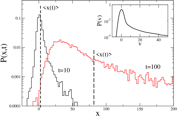
Figure 3: Main frame: Semi-Log plot of $P(x,t)$ at $t=10$ (black histogram), and $t=100$ (red histogram) for superdiffusive dynamics with $g=5/2$ and constant external field $\mathcal{E}=1.5$. Let us notice that for increasing time the typical (most frequent) value, and the mean (indicated with a vertical dashed line) of the distribution become increasingly different for growing times. The increasing average value of the distribution is due to the arising of a power-law tail for $P(x,t)$. Inset: Semi-Log plot of the velocity PDF $P(v)$.

The study of the Einstein relation on a state with non-zero current induced by a constant field $\mathcal{E}$ allows us to show that there is some “anomaly” in the dynamics also when the exponent of the power law distribution of times is $g>3$. More precisely, when $3<g<5$, at equilibrium, i.e. in the absence of current, a fluctuation-dissipation experiment would not show any anomaly in the dynamics, because $\langle[\delta x(t)]^{2}\rangle\sim\langle x(t)\rangle_{\mathcal{E}}$. On the other hand, the same experiment done out of equilibrium, i.e. comparing the MSD around the drift with the drift itself, shows an evident violation

$$\frac{\langle[\delta x(t)]^{2}\rangle_{\mathcal{E}}}{\langle x(t)\rangle_{\mathcal{E}}}\sim t^{5-g}.$$ (21)

4 Conclusions

The present study concerns the comparison of the drift of a probe particle in the presence of an external field with its MSD, measured either in the presence or in the absence of the external perturbation. The outcome of our study is that, while for a Lévy walk process the equilibrium fluctuation-dissipation relation is always valid [8], the situation is very different in the out-of-equilibrium case, where we have a breaking of the Einstein relation. In particular, we find that the standard fluctuation-dissipation relation can be recovered by replacing the MSD with the diffusion around the average current $\langle x^{2}(t)\rangle_{\mathcal{E}}-\langle x(t)\rangle_{\mathcal{E}}^{2}$, as it happens for standard random walks, only for values of the exponent $g>5$. This is a new an unexpected result, since already for $g>3$ we observe a simple diffusive dynamics at equilibrium, even if the $P(x,t)$ is non-Gaussian. The non-Gaussian nature of the distribution of displacements emerges for $3<g<5$ only through a “response experiment” in presence of some currents.

As shown in Fig. 3, the violation of the fluctuation-dissipation relation for $g<5$ comes together with a strongly asymmetric shape of the $P(x,t)$ for large times. Let us note that such a mechanism, namely a transport mechanism which do not correspond to a uniform shifts of the $P(x,t)$, is peculiar not only of this superdiffusive model, but has already been observed in the context of subdiffusive dynamics [11].

References

References

- [1] R Kubo. The fluctuation-dissipation theorem. Rep. Prog. Phys., 29:255, 1966.
- [2] J P Bouchaud and A Georges. Anomalous diffusion in disordered media: Statistical mechanisms, models and physical applications. Phys. Rep., 195:127, 1990.
- [3] Q Gu, E A Schiff, S Grebner, F Wang, and R Schwarz. Non-gaussian transport measurements and the Einstein relation in amorphous silicon. Phys. Rev. Lett., 76:3196, 1996.
- [4] P Castiglione, A Mazzino, P Muratore-Ginanneschi, and A Vulpiani. On strong anomalous diffusion. Physica D, 134:75, 1999.
- [5] R Metzler and J Klafter. The random walk’s guide to anomalous diffusion: a fractional dynamics approach. Phys. Rep., 339:1, 2000.
- [6] R Burioni and D Cassi. Random walks on graphs: ideas, techniques and results. J. Phys. A:Math. Gen., 38:R45, 2005.
- [7] J Klafter and I M Sokolov. First steps in random walks. Oxford University Press, 2011.
- [8] E Barkai and V N Fleurov. Generalized Einstein relation: A stochastic modeling approach. Phys. Rev. E, 58:1296, 1998.
- [9] S Jespersen, R Metzler, and H C Fogedby. Lévy flights in external force fields: Langevin and fractional Fokker-Planck equations and their solutions. Phys. Rev. E, 59:2736, 1999.
- [10] R Metzler, E Barkai, and J Klafter. Anomalous diffusion and relaxation close to thermal equilibrium: A fractional Fokker-Planck equation approach. Phys. Rev. Lett, 82:3563, 1999.
- [11] D Villamaina, A Sarracino, G Gradenigo, A Vulpiani, and A Puglisi. On anomalous diffusion and the out of equilibrium response function in one-dimensional models. J. Stat. Mech., page L01002, 2011.
- [12] D Villamaina, A Puglisi, and A Vulpiani. The fluctuation-dissipation relation in sub-diffusive systems: the case of granular single-file diffusion. J. Stat. Mech., page L10001, 2008.
- [13] E Barkai and J Klafter. Anomalous diffusion in the strong scattering limit: A Lévy walk approach. In S Benkadda and G M Zaslavsky, editors, Chaos, Kinetics and Nonlinear Dynamics in Fluids and Plasmas, volume 511 of Lectures Notes in Physics, Berlin Heidelberg, 1998. Springer-Verlag.
- [14] M H Ernst. Nonlinear model-Boltzmann equations and exact solutions. Phys. Rep., 78:1, 1981.
- [15] P Levitz. From Knudsen diffusion to Lévy walks. Europhys. Lett., 39:593, 1997.
- [16] K H Andersen, P Castiglione, A Mazzino, and A Vulpiani. Simple stochastic models showing strong anomalous diffusion. Eur. Phys. J. B, 18:447, 2000.
- [17] A Alastuey and J Piasecki. Approach to a stationary state in an external field. J. Stat. Phys., 139:991, 2010.
- [18] G Gradenigo, A Puglisi, A Sarracino, and U Marini Bettolo Marconi. Nonequilibrium fluctuations in a driven stochastic Lorentz gas. Phys. Rev. E, 85:031112, 2012.
- [19] M Barbier and E Trizac. Field induced stationary state for an accelerated tracer in a bath. arXiv:1203.6759.
- [20] U Marini Bettolo Marconi, A Puglisi, L Rondoni, and A Vulpiani. Fluctuation-dissipation: Response theory in statistical physics. Phys. Rep., 461:111, 2008.
- [21] R Burioni, L Caniparoli, and A Vezzani. Lévy walks and scaling in quenched disordered media. Phys. Rev. E, 81:060101, 2010.