Analytical Bounds between Entropy and Error Probability in Binary Classifications
Abstract
The existing upper and lower bounds between entropy and error probability are mostly derived from the inequality of the entropy relations, which could introduce approximations into the analysis. We derive analytical bounds based on the closed-form solutions of conditional entropy without involving any approximation. Two basic types of classification errors are investigated in the context of binary classification problems, namely, Bayesian and non-Bayesian errors. We theoretically confirm that Fano’s lower bound is an exact lower bound for any types of classifier in a relation diagram of “error probability vs. conditional entropy”. The analytical upper bounds are achieved with respect to the minimum prior probability, which are tighter than Kovalevskij’s upper bound.
Index Terms:
Entropy, error probability, Bayesian errors, analytical, upper bound, lower boundI Introduction
In information theory, the relations between entropy and error probability are one of the important fundamentals. Among the related studies, one milestone is Fano’s inequality (also known as Fano’s lower bound on the error probability of decoders), which was originally proposed in 1952 by Fano, but formally published in 1961 [1]. It is well known that Fano’s inequality plays a critical role in deriving other theorems and criteria in information theory [2][3][4]. However, within the research community, it has not been widely accepted exactly who was first to develop the upper bound on the error probability [5]. According to [6] [7], Kovalevskij [8] was possibly the first to derive the upper bound of the error probability in relation to entropy in 1965. Later, several researchers, such as Chu and Chueh in 1966 [9], Tebbe and Dwyer III in 1968 [10], Hellman and Raviv in 1970 [11], independently developed upper bounds.
The upper and lower bounds of error probability have been a long-standing topic in studies on information theory [12] [13] [14] [15] [16] [18] [19] [20][6] [7]. However, we consider two issues that have received less attention in these studies:
I. What are the “analytical bounds” for which approximations have not been applied in the derivation?
II. What is the interpretation of each bound or some key points in a given diagram of entropy and error probability?
On the first issue, we define “analytical bounds” to be those derived from closed-form solutions, rather than from inequality approximations. Generally, exact bounds are desirable from the viewpoint of theory and applications. The second issue suggests the need for a better understanding of the bounds in the relation of entropy and error probability. For example, some key points located at the bounds could show the specific interpretations for theoretical insights or application meanings.
The above issues forms the motivation behind this work. We establish analytical bounds based on closed-form solutions. Furthermore, we study the bounds in a wider range of error type, i.e., Bayesian and non-Bayesian. Non-Bayesian errors are also of importance because most classifications are realized within this category. We take classifications as a problem background since it is more common and understandable from our daily-life experiences. We intend to simplify settings within binary states and Shannon entropy definitions so that the analytical-principle approach is highlighted. Based on this principle, one is able to extend the study to more general classification settings, such as multiple-class (or multihypothesis) problems, and on other definitions of entropy, such as Rényi entropy.
The rest of this paper is organized as follows. In Section II, we present related works on the bounds. For a problem background of classifications, several related definitions are given in Section III. The analytical bounds are given and discussed for Bayesian and non-Bayesian errors in Sections IV and V, respectively. Interpretations to some key points are presented in Section VI. Finally, in Section VII we conclude the work and present some discussions.
II Related Works
Two important bounds are introduced first, which form the baselines for the comparisons with the analytical bounds. They were both derived from inequality conditions[1][8]. Suppose the random variables and representing input and output messages (out of possible messages), and the conditional entropy representing the average amount of information lost on when given . Fano’s lower bound [1] is given in a form of:
where is the error probability, and is the associated binary Shannon entropy defined by [21]:
The base of the logarithm is 2 so that the units are “bits”.
The upper bound is given by Kovalevskij [8] in a piecewise linear form:
| (3) |
For a binary classification (), Fano-Kovalevskij bounds become:
where is an inverse of .
Several different bound diagrams between error probability and entropy have been reported in literature. The initial difference is made from the entropy definitions, such as Shannon entropy in [12][14][22][23], and Rényi entropy in [15][6][7]. The second difference is the selection of bound relations, such as “ vs. ” in [12], “ vs. ” in [14] [15][6] [7], “ vs. ” in [24], and “ vs. ” in [22], where is the accuracy rate, and are the mutual information and normalized mutual information, respectively, between variables and . Wang and Hu [22] was the first to derive the analytical relations of mutual information with respect to accuracy, precision, and recall, and their analytical bounds. However, they did not consider the Bayesian error constraint. When the Bayesian error constraint was added into the bound relation in [23], the upper bound from [8] is not analytical one. Because the existing bounds are derived from inequality with approximations, some investigations [17] [18] [20] have been reported on the improvement of bound tightness.
III Related Definitions
Binary classifications are considered in this work. A theoretical derivation of relations between entropy and error probability, is achieved based on the joint probability in classifications, where is the true (or target) state within two classes, and is the classification output. The simplified notations for are used in this work. Several definitions are given below.
Definition 1 (Joint probability in binary classifications): In a context of binary classifications, the joint probability is defined in a generic setting as:
where and are the prior probabilities of Class 1 and Class 2, respectively; their associated error probabilities are denoted by and , respectively. For the Bayesian decision, and are always known. The constraints in eq. (5) are given:
Definition 2 (Bayesian error and non-Bayesian error): “Bayesian error” is defined to be the theoretically lowest error in classifications [25], and denoted by . Hence, the other errors are “non-Bayesian errors”, and denoted by for the same probability distributions).
Definition 3 (Error probability calculation): In binary classifications, error probabilities are calculated from the same formula:
where is also denoted an error variable with no distinction between error types.
Definition 4 (Minimum and maximum error bounds in classifications): Classifications suggest the minimum error bound as:
where the subscript “min” denotes the minimum value. The maximum error bound for Bayesian error in binary classifications is [23]:
where the symbol “min” denotes a “minimum” operation. For non-Bayesian error, its maximum error bound becomes
Definition 5 (Admissible area, point and their properties in a diagram of entropy and error probability): In a given diagram of entropy and error probability, we define the area enclosed by the bounds to be “admissible area”, if every point inside the area can be possibly realized from classifications. we call those points to be “admissible points”. If a point is unable to be realized from classifications, it is a “non-admissible point”. A non-admissible point can only be located at or outside the boundary of the admissible area. If every point located on the boundary is admissible, we call this admissible area “closed”. If one or more points at the boundary are non admissible, the area is said “open”.
IV Analytical upper and lower bounds for Bayesian errors
All analytical bounds are derived from a closed-form relation of conditional entropy and error probabilities (see Appendix A). The analytical lower bound for Bayesian errors is:
| (11) |
where is the conditional entropy for the random variables and , and is called the “analytical lower bound function” (or “analytical lower bound” for short) and satisfies the following relations with respect to the error variable :
| (12) |
The analytical upper bound is given by:
| (13) |
where is the “analytical upper bound function” and for which the following relation holds:
| (14) |
In eq. (14) is known, because for Bayesian classifications and are given information.
Fig. 1 depicts three analytical upper bounds together with Fano’s lower bound and Kovalevskij’s upper bound in the graph of “ vs. ”. Several findings can be observed from the novel upper bounds.
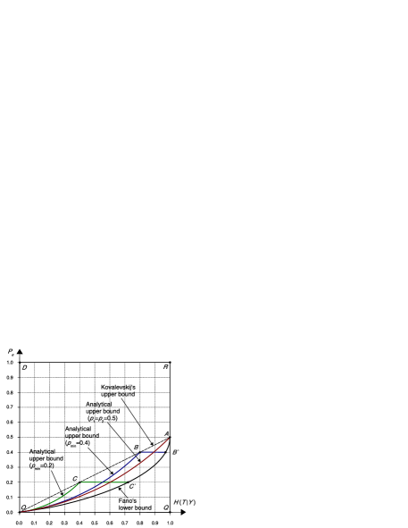
I. If , the analytical upper bounds are formed by one curve and one line. These are lower than Kovalevskij’s upper bound except for two specific points: the original point, , and one corner point, or , in Fig. 1.
II. If , the analytical upper bound becomes a single curve, which is also lower than Kovalevskij’s upper bound, except at the two end-points, points and .
III. The analytical upper bounds, either curved or linear, are controlled by .
IV. The admissible area in Bayesian decision is closed. Its shape changes depending on the value of . For example, the area enclosed by the two-curve-one-line boundary, “” in Fig. 1, corresponds to classifications with . The line boundary shows the maximum error for Bayesian decisions, , in binary classifications [23].
Interpretations are given below to the analytical bounds in the context of binary classifications. Similar discussions on some specific points are gvien in Section VI.
Fano’s lower bound: In [2], a marginal probability distribution is applies for explaining the equality of Fano’s lower bound (see eq. (2-144), [2]):
| (15) |
Because we derive the bound based on joint probability distributions in (5), novel explanations can be obtained. A generic classification setting can represent this bound:
| (16) |
The setting above is derived based on the minimum relations (or Property 7 in [26]). Eq. (16) describes an extremal property in the relations of entropy and error probability, but is expressed between the error probabilities.
Based on eq. (16), a specific classification setting can be obtained, in which one is to classify a minority class (say, Class 2) into a majority class (Class 1):
| (17) |
Eq. (17) will result in a zero value for the mutual information, which implies “no correlation” [25] between two variables and , or “zero information” [27] from the classification decisions. It also indicates the “statistically independent” [2] between two variables. In [23], Hu demonstrated that Bayesian classifiers will obtain such solutions for when processing extremely-skewed classes with no cost terms given. One can also observe that eq. (17) is equivalent to (15) when .
Analytical upper bound: Supposing , a specific classification setting can be obtained for representing this bound:
| (18) |
Eq. (18) suggests the generic conditions, if and , for another extremal property in the relations of entropy and error probability. Hence, the analytical upper bound function corresponds to a zero value for the conditional probability, or the maximum value for the mutual information.
V Analytical upper and lower bounds for non-Bayesian errors
In a context of classification problems, Bayesian errors can be realized only if one has exact information about all probability distributions [25]. The assumption above is generally impossible in real applications. Therefore, the analysis of non-Bayesian errors also presents significant interests in studies.
The Fano’s lower bound will be effective for all classifications. The bound is general and independent of error type and information about and . If no information is given about and , we obtain a “general upper bound” for non-Bayesian errors in the form:
| (19) |
which is a mirror of Fano’s lower bound with mirror axis along . If one has information about and , the analytical upper bound of is
| (20) |
where is the “upper bound of ” and calculated from:
| (21) |
The analytical upper bound described in (14) also forms a “mirrored analytical upper bound”, which will be effective for .
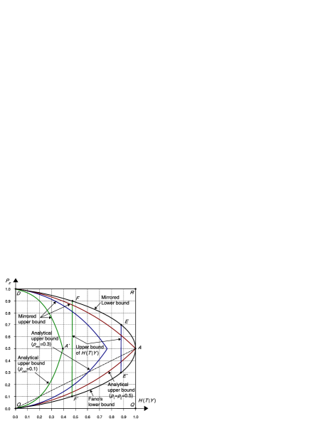
From the graph of “ vs. ” (Fig. 2), observations for non-Bayesian errors can also be summarized as follows:
I. In general, if no information exists about and , the admissible area is formed by Fano’s lower bound, its mirrored bound, and the axis of , that is, the two-curve-one-line boundary “” in Fig. 2. This area covers all other admissible areas formed from analytical bounds for which information about and is applied.
II. If and are known, the admissible area will be formed from the analytical upper bound, its mirrored bound, and the upper bound . The area is controlled by . For example, if , the area is enclosed by the four-curve-one-line boundary “” in Fig. 2. However, if , two admissible areas are specifically formed. Their two-curve boundaries are “” and “”, respectively.
III. All admissible areas, whether with or without information of and , are closed. The areas are formed differently with respect to the given information. The more information available, the tighter the bounds become, or the smaller the admissible areas become. In general, non-Bayesian error can be higher than Kovalevskij’s bound.
General upper bound of non-Bayesian errors: For non-Bayesian classifications, eq. (5) with condition describes a general classification setting to represent the general upper bound. Two specific settings can be obtained for demonstrations. One setting is described by eq. (17) with . The other setting is
| (22) |
Mirrored analytical upper bound: A mirrored analytical upper bound is formed for non-Bayesian error with the condition that and are known. This bound in fact serves as a lower bound for . Suppose , a specific setting in classifications can be found for representing the mirrored bound:
| (23) |
VI Interpretations to some key points
Further interpretations are given to the key points shown in Fig. 1 and Fig. 2. Those key points may hold special features in classifications.
Point O: This point represents a zero value of . It also suggests a “perfect classification” without any error () by a specific setting of the joint probability:
Point A: This point represents maximum ranges of for “class-balanced” classifications (). Three specific classification settings can be obtained for representing this point. The two settings are actually “no classification”:
The other one is a “random guessing”:
Point D: This point occurs for non-Bayesian classifications in a form of:
In this case, one can exchange the labels for a perfect classification.
Points B (or C) and (or ): Suppose . The specific setting is:
for Point when (or Point when ), and two specific settings for Point (or Point ) are:
or
Points E (or F) and (or ): Suppose . The specific setting is:
for Point when (or Point when ), and eq. (30) for Point (or ) on the given value of .
Point : Suppose . The specific setting for Point is:
Points Q and R: The two points are specific due to their positions in the diagrams. For both types of errors, they are all considered to be “non-admissible points” in the diagrams, because no setting exists in binary classifications which can represent the points.
VII Final remarks
This work investigates into analytical bounds between entropy and error probability. Two specific schemes are applied in the theoretical derivation. One scheme is the utilization of joint probability distributions, on which more general interpretations can be obtained for understanding the bounds. The other scheme is the closed-form solution of the maximization or minimization to the related functions. We derived the analytical bounds for both types of Bayesian errors and non-Bayesian ones. While a new interpretation is given to Fano’s lower bound, the analytical upper bounds are achieved which show tighter than Kovalevskij’s upper bound.
To emphasize the importance of the study, we present discussions below on the selection of learning targets between error and entropy from the perspective of machine learning. The analytical bounds derived in this work provide a novel solution to link both learning targets in the related studies. Error-based learning is more conventional because of its compatibility with our intuitions in daily life, such as “trial and error”. Significant studies have been reported under this category. In comparison, information-based learning [28] is new and uncommon in applications, such as classifications. Entropy is not a well-accepted concept related to our intuition in decision making. This is one of the reasons why the learning target is chosen mainly based on error, rather than on entropy. However, we consider that error is an empirical concept, whereas entropy is generally more theoretical. In [29], we demonstrated that entropy can deal with both concepts of “error” and “reject” in abstaining classifications. Information-based learning [28] presents a promising and wider perspective for exploring and interpreting learning mechanisms.
When considering all sides of the issues stemming from machine learning studies, we believe that “what to learn” is a primary problem. However, it seems that more investigation is focused on the issue of “how to learn”. Moreover, in comparison with the long-standing yet hot theme of “feature selection”, little study has been done from the perspective of “learning target selection”. We propose that this theme should be emphasized in the study of machine learning. Hence, the relations studied in this work are very important and crucial to the extent that researchers, using either error-based or entropy-based approaches, are able to reach a better understanding about its counterpart.
Appendix A Proofs of the analytical bounds
For a binary classification, a closed-form relation of conditional entropy and error probabilities is derived from the joint probability (5):
Based on eq. (A1), the analytical functions of lower bound and upper bound should be derived from the following definitions, respectively:
The meanings of lower and upper are exchanged in (A2) and (A3) respectively, because the input variable is in the derivations. A single independent parameter is given to , which is assumed to be known in the derivations.
However, in the background of binary classifications, the function in (A1) has two independent variables, and . This feature causes a difficulty in the direct derivation of (A2) or (A3) based on a single variable function . The difficulty is the multiple solutions of and to the same bound, which makes the derivation to be tedious. For overcoming this difficulty, we adopt Maple™9.5 (a registered trademark of Waterloo Maple, Inc.) for implementing the derivations. Using the Maple code shown in Appendix B, one is able to confirm the derivations easily for the multiple-to-one relations of the bound.
Proof:
On the analytical lower bound function :
From information theory [2], one can have the following conditions for mutual information:
Hence, eq. (A1) describes that, when , one can have the maximum results of . We can show that the generic classification setting in eq. (16) will result in the condition of . Using the Maple code, one can substitute either condition from (16) into (A1), and always arrive at the same results on and the analytical lower bound function in terms of and . ∎
Proof:
On the analytical upper bound function :
Eq. (A1) suggests that the maximum solution of should be equivalent. For achieving a single-variable function in (A3), we need to solve the following problem first:
where is described implicitly by two independent variables and . Due to high complexity of the nonlinearity in , we are unable to obtain the direct relation between and . Therefore, we solve the problem of (A5) by examining the differential function of with respect to :
where we consider and as the constants. Suppose the condition , one can prove that (A6) is always negative and without singularity. Hence, is a monotonously decreasing function with respect to for the given condition. The maximum will require the smallest . From and the given in (A5), one can derive the solutions and . The specific classification setting associated to the solutions is shown in (18). For the other conditions with the same value of , one can always obtain the same value on the maximum of . The analytical upper bound function will be always the same in terms of and . ∎
The proof of mirrored bounds can be obtained directly in the similar principle, and is neglected here.
Appendix B Maple code for the derivations
> #  Maple code for deriving the analytical lower bound
> restart; # Clean the memory
> # Shannon entropy
> HT:=-p1*log[2](p1)-p2*log[2](p2);
> # Terms of joint probability
> p11:=(p1-e1);p12:=e1;p22:=p2-e2;p21:=e2;
> # For the generic setting in (16)
> e1:=p1*(p2-e2)/p2;p1:=1-p2;
> # Intermediate variables
> q1:=p11+p21;q2:=p12+p22;
> # Mutual information
> MI:=p11*log[2](p11/q1/p1)+p12*log[2](p12/q2/p1);
> MI:=MI+p22*log[2](p22/q2/(1-p1))+p21*log[2](p21/q1/(1-p1));
> MI:=simplify(MI,ln);    # Solution of mutual information
                            MI := 0
> # The analytical lower bound function
> HTY:=simplify((HT-MI),ln);
> # Display of the lower bound function in terms of e and p2
                     (1 - p2) ln(1 - p2)   p2 ln(p2)
            HTY := - ------------------- - ---------
                            ln(2)            ln(2)
> #  Maple code for deriving the analytical upper bound
> restart; # Clean the memory
> # Shannon entropy
> HT:=-p1*log[2](p1)-p2*log[2](p2);
> # Terms of joint probability
> p11:=(p1-e1);p12:=e1;p22:=p2-e2;p21:=e2;
> # For error variable
> e1:=e-e2;p1:=1-p2;
> # Intermediate variables
> q1:=p11+p21;q2:=p12+p22;
> # Mutual information
> MI:=p11*log[2](p11/q1/p1)+p12*log[2](p12/q2/p1);
> MI:=MI+p22*log[2](p22/q2/(1-p1))+p21*log[2](p21/q1/(1-p1));
> MI_dif:=simplify(combine(diff(MI,e),ln, symbolic));
> # Display of diffential function of MI in (A6)
                    /  (-1 + p2 + e - 2 e2) (e - e2)   \
                  ln|----------------------------------|
                    \(-1 + p2 + e - e2) (e - 2 e2 + p2)/
        MI_dif := --------------------------------------
                                  ln(2)
> # For the generic setting in (18)
> e1:=e;e2:=0;p1:=1-p2;
> # Intermediate variables
> q1:=p11+p21;q2:=p12+p22;
> # Mutual information
> MI:=p11*log[2](p11/q1/p1)+p12*log[2](p12/q2/p1);
> # Neglect one term below from the entropy definition of 0*log(0)=0
> MI:=MI+p22*log[2](p22/q2/(1-p1));
> # The analytical upper bound function
> HTY:=combine(simplify(combine(simplify(HT-MI),ln,symbolic)));
> # Display of the upper bound function in terms of e and p2
                       /e + p2\       /e + p2\
                  p2 ln|------| + e ln|------|
                       \  p2  /       \  e   /
            HTY:= ----------------------------
                             ln(2)
Acknowledgments
This work is supported in part by NSFC (No. 61075051 for BG and No. 60903089 for HJ).
References
- [1] R.M. Fano, Transmission of Information: A Statistical Theory of Communication. New York: MIT, 1961.
- [2] T.M. Cover and J.A. Thomas, Elements of Information Theory. 2nd eds., New York:John Wiley, 2006.
- [3] S. Verdú, “Fifty years of Shannon theory,” IEEE Trans. Inform. Theory, vol. 44, pp. 2057–2078, 1998.
- [4] R.W. Yeung, A First Course in Information Theory. London:Kluwer Academic, 2002.
- [5] J. D. Golić, “Comment on ‘Relations between entropy and error probability’,” IEEE Trans. Inform. Theory, vol. 45, p. 372, 1999.
- [6] I. Vajda and J. Zvárová, “On generalized entropies, Bayesian decisions and statistical diversity,” Kybernetika, pp. 675–696, 2007.
- [7] D. Morales and I. Vajda: “Generalized Information Criteria for Optimal Bayes Decisions”. Research Report, No. 2274, Institute of Information Theory and Automation, Academy of Sciences of the Czech Republic, 2010.
- [8] V.A. Kovalevskij, “The problem of character recognition from the point of view of mathematical statistics,” Character Readers and Pattern Recognition, pp. 3–30, New York:Spartan, 1968. Russian edition 1965.
- [9] J. T. Chu and J. C. Chueh, “Inequalities between information measures and error probability,” J. Franklin Inst., vol. 282, pp. 121–125, 1966.
- [10] D. L. Tebbe and S. J. Dwyer III, “Uncertainty and probability of error,” IEEE Trans. Inform. Theory., vol. 16, pp. 516–518, 1968.
- [11] M. E. Hellman and J. Raviv, “Probability of error, equivocation, and the Chernoff bound,” IEEE Trans. Inform. Theory., vol. 16, pp. 368–372, 1970.
- [12] C.H. Chen, “Theoretical comparison of a class of feature selection criteria in pattern recognition,” IEEE Trans. Comput., vol. C-20, pp. 1054–1056, 1971.
- [13] M. Ben-Bassat and J. Raviv, “Renyi’s entropy and the prbability of Error,” IEEE Trans. Inform. Theory, vol. 24, pp. 324–330, 1978.
- [14] J. D. Golić, “On the relationship between the information measures and the Bayes probability of error,” IEEE Trans. Inform. Theory, vol. 35, pp. 681–690, 1987.
- [15] M. Feder and N. Merhav, “Relations between entropy and error Probability,” IEEE Trans. Inform. Theory, vol. 40, pp. 259–266, 1994.
- [16] T.S. Han and S. Verdú, “Generalizing the Fano inequality,” IEEE Trans. Inform. Theory, vol. 40, pp.1247–1251, 1994.
- [17] I. J. Taneja, “Generalized error bounds in pattern recognition,” Pattern Recognition Letters 3, vol. 3, 361–368, 1985.
- [18] H.V. Poor and S. Verdú, ”A Lower bound on the probability of error in multihypothesis testing,” IEEE Trans. Inform. Theory, vol. 41, pp. 1992–1994, 1995.
- [19] P. Harremoës and F. Topsøe, ”Inequalities between entropy and index of coincidence derived from information diagrams,” IEEE Trans. Inform. Theory, vol. 47, pp. 2944–2960, 2001.
- [20] D. Erdogmus, and J.C. Principe, “Lower and upper bounds for misclassification probability based on Renyi’s information,” Journal of VLSI Signal Processing, vol. 37, pp. 305–317, 2004.
- [21] C.E. Shannon, “A mathematical theory of communication”, Bell System Technical Journal, vol. 27, pp. 379–423 and pp. 623–656, 1948.
- [22] Y. Wang and B.-G. Hu, “Derivations of normalized mutual information in binary classifications,” Proceedings of the 6th International Conference on Fuzzy Systems and Knowledge Discovery, pp. 155–163, 2009.
- [23] B.-G. Hu, “What are the differences between Bayesian classifiers and mutual-information classifiers?” Preprint available: http://arxiv.org/abs/1105.0051v2, 2012.
- [24] T. Eriksson, S. Kim, H.-G. Kang, and C. Lee, “An information-theoretic perspective on feature selection in speaker recognition,” IEEE Signal Processing Letter, vol. 12, pp. 500–503, 2005.
- [25] R.O. Duda, P.E. Hart, and D. Stork, Pattern Classification. 2nd eds., New York: John Wiley, 2001.
- [26] B.-G. Hu and Y. Wang, “Evaluation criteria based on mutual information for classifications including rejected class,” Acta Automatica Sinica, vol. 34, pp. 1396–1403, 2008.
- [27] D.J.C. Mackay, Information Theory, Inference, and Learning Algorithms. Cambridge:Cambridge University Press, 2003.
- [28] J.C. Principe, Information Theoretic Learning: Renyi’s Entropy and Kernel Perspectives. New York: Springer, 2010.
- [29] B.-G. Hu, R. He, and X.-T, Yuan, “Information-theoretic measures for objective evaluation of classifications,” Acta Automatica Sinica, vol. 38, pp. 1160–1173 2012.