Estimating sufficient reductions of the predictors in abundant high-dimensional regressions

Abstract

We study the asymptotic behavior of a class of methods for sufficient dimension reduction in high-dimension regressions, as the sample size and number of predictors grow in various alignments. It is demonstrated that these methods are consistent in a variety of settings, particularly in abundant regressions where most predictors contribute some information on the response, and oracle rates are possible. Simulation results are presented to support the theoretical conclusion.

, and

t1Supported by NSF Grants DMS-10-07547 and DMS-11-05650.

t2Supported by NSF Grant DMS-11-05650.

1 Introduction

There are many facets to the analysis of data in high dimensions, depending on the type of application, some relying on dimension reduction, others relying on variable selection and a few employing both tactics. There has been considerable interest in dimension-reduction methods for the regression of a real response $Y$ on a random vector of predictors ${\mathbf{X}}\in{\mathbb{R}}^{p}$ since the introduction of sliced inverse regression [SIR; Li (1991)] and sliced average variance estimation [SAVE; Cook and Weisberg (1991)]. A common goal of these and many other methods is to reduce the dimension of the predictor vector without loss of information about the response. The aim is to estimate a reduction ${\mathbf{R}}\dvtx{\mathbb{R}}^{p}\rightarrow{\mathbb{R}}^{d}$, $d\leq p$, with the property that $Y\perp\perp{\mathbf{X}}|{\mathbf{R}}({\mathbf{X}})$ or, equivalently, ${\mathbf{X}}|(Y,{\mathbf{R}}({\mathbf{X}}))\sim{\mathbf{X}}|{\mathbf{R}}({\mathbf{X}})$ [Cook (2007)]. In this way ${\mathbf{R}}$ is sufficient because it captures all the information about $Y$ that is available from ${\mathbf{X}}$. Sufficient reductions are not determined uniquely by this definition because any bijective transformation of ${\mathbf{R}}$ is also sufficient.

Nearly all methods for sufficient dimension reduction (SDR) restrict attention to the class of linear reductions, which arise naturally in many contexts. Linear reduction can be represented conveniently in terms of the projection ${\mathbf{P}}_{{\mathcal{S}}}{\mathbf{X}}$ of ${\mathbf{X}}$ onto a subspace ${\mathcal{S}}\subseteq{\mathbb{R}}^{p}$. If $Y\perp\perp{\mathbf{X}}|{\mathbf{P}}_{{\mathcal{S}}}{\mathbf{X}}$, then ${\mathcal{S}}$ is called a dimension-reduction subspace. Under mild conditions the intersection of any two dimension-reduction subspaces is again a dimension-reduction subspace and that being so the central subspace $\mathcal{S}_{Y|{\mathbf{X}}}$, defined as the intersection of all dimension-reduction subspaces, is taken as the inferential target [Cook (1994, 1998)]. A minimal sufficient linear reduction is then of the form ${\mathbf{R}}({\mathbf{X}})=\bolds{\eta}^{T}{\mathbf{X}}$, where $\bolds{\eta}$ is any basis for $\mathcal{S}_{Y|{\mathbf{X}}}$.

SDR has a long history of successful application and is still an active research area. Recent novel SDR methods include likelihood-based sufficient dimension reduction [Cook and Forzani (2009)], kernel dimension reduction [Fukumizu, Bach and Jordan (2009)], shrinkage inverse regression estimation [Bondell and Li (2009)], dimension reduction for nonelliptically distributed predictors [Li and Dong (2009), Dong and Li (2010)], cumulative slicing estimation [Zhu, Zhu and Feng (2010)], dimension reduction for survival models [Xia, Zhang and Xu (2010)] and dimension reduction for spatial point processes [Guan and Wang (2010)]. This body of work reflects three different but related frontiers in SDR: extensions that require progressively fewer assumptions, development of likelihood-based methods and adaptations for specific areas of application. Almost all SDR methods rely on traditional asymptotic reasoning for support, letting the sample size $n\rightarrow\infty$ with $p$ fixed. They nearly all require the inverse of a $p\times p$ sample covariance matrix and thus application is problematic when $n<p$. Since accurate estimation of a general $p\times p$ covariance matrix can require $n\gg p$ observations, it has seemed inevitable that SDR methods would encounter estimation problems when $n$ is not sufficiently large. Chiaromonte and Martinelli (2002), Li and Li (2004) and others circumvented these issues by performing reduction in two stages, first replacing the $p$ predictors with $p^{*}\ll n$ principal components and then applying an SDR method to the regression of the response on the selected $p^{*}$ components. However, recent results on the eigenvectors of sample covariance matrices in high-dimensional settings raise questions on the value of such two-stage methods [see, e.g., Johnstone and Lu (2009)]. Cook, Li and Chiaromonte (2007) proposed an SDR method that avoids computation of inverses and reduces to partial least squares in a special case. Chun and Keleş (2010) showed recently that the partial least squares estimator of the coefficient vector in the linear regression of $Y$ on ${\mathbf{X}}$ is inconsistent unless $p/n\rightarrow 0$ and this raises questions about the behavior of the Cook et al. SDR estimator when $n$ is not large relative to $p$. Li and Yin (2008) used the least squares formulation of sliced inverse regression originated by Cook (2004) to develop a regularized version that allows $n<p$ and achieves simultaneous predictor selection and dimension reduction. This seems to be a promising method, but its asymptotic properties are unknown and it may not work well when the regression is not sparse. Wu and Li (2011) studied the asymptotic properties of a family of SDR estimators, using a SCAD-type penalty for variable selection in sparse regressions where the number of relevant variables is fixed as $p\rightarrow\infty$. Their method requires that $p/n\rightarrow 0$ for consistency.

While sparsity is an important concept in high-dimensional regression, not all high-dimensional regressions are sparse. For example, near-infrared reflectance is often measured at many wavelengths to predict the composition of matter, like the protein content of a grain. There is not normally an expectation that only a few wavelengths are needed to predict content. While some wavelengths may be better predictors than others, it is the cumulative information provided by many wavelengths that is often relevant. Partial least squares has been the dimension-reduction method of choice in this type of regression. The regressions implied by this and other nonsparse applications share similar characteristics: (1) the predictor vectors are high-dimensional and typical area-specific analyses have employed some type of dimension reduction; (2) while assessing the relative importance of the predictors may be of interest, prediction is the ultimate goal; (3) information on the response is thought to accumulate, albeit perhaps slowly, as predictors are added, and (4) sparsity is not a driving notion.

In this article we introduce a family of SDR methods for studying high-dimensional regressions that differs from past approaches in at least three important ways. First, we do not require sparsity but rather we emphasize abundant regressions where most of the predictors contribute some information about the response. In the logic of Friedman et al. (2004), the bet-on-sparsity principle arose because, to continue the metaphor, there is otherwise little chance of a reasonable payoff. We show in contrast that reasonable payoffs can be obtained in abundant regressions with prediction as the ultimate goal, leading to a contrasting bet-on-abundance principle. Second, SDR studies have largely focused on properties of estimators of $\mathcal{S}_{Y|{\mathbf{X}}}$. We bypass this step and instead consider the limiting behavior of estimators of the sufficient reduction ${\mathbf{R}}({\mathbf{X}})$ itself, assuming that the dimension $d$ of ${\mathbf{R}}$ is fixed. More specifically, letting $\widehat{{\mathbf{R}}}$ denote an estimated reduction, we establish rates of convergence in the following sense. Let ${\mathbf{X}}_{N}$ denote a new observation on ${\mathbf{X}}$. If $\widehat{{\mathbf{R}}}({\mathbf{X}}_{N})-{\mathbf{R}}({\mathbf{X}}_{N})=O_{p}(r(n,p))$ and if $r(n,p)\rightarrow 0$ as $n,p\rightarrow\infty$, then $\widehat{{\mathbf{R}}}({\mathbf{X}}_{N})$ is consistent for ${\mathbf{R}}({\mathbf{X}}_{N})$ and its convergence rate is at least $r^{-1}$. Third, we integrate recent work on the estimation of high-dimensional covariance matrices into our approach. In particular, we estimate a critical matrix of weights by using sparse permutation invariant covariance estimation (SPICE) as developed by Rothman et al. (2008).

In sum, by considering the reduction ${\mathbf{R}}$ itself rather than the central subspace $\mathcal{S}_{Y|{\mathbf{X}}}$, we both introduce a novel viewpoint for addressing dimension reduction and develop theoretically grounded SDR methodology for $n<p$ regressions where other methods either have no asymptotic support or must necessarily fail.

We describe the model for our study and its sufficient reduction in Section 2. The class of estimators that we use is described in Section 3, and stabilizing restrictions are presented in Section 4. Sections 5 and 6 contain theoretical conclusions for selected estimators from the class described in Section 3. Simulation results are presented in Sections 5.2 and 7. We turn to a spectroscopy application in Section 8 and a concluding discussion is given in Section 9. All proofs and additional simulation results are available in a supplemental article [Cook, Forzani and Rothman (2012)].

The following notational conventions will be used in our exposition. We use ${\mathbb{R}}^{p\times q}$ to denote the collection of all real $p\times q$ matrices. We use $\|{\mathbf{A}}\|$ and $\|{\mathbf{A}}\|_{F}$ to denote the spectral and Frobenius norms of ${\mathbf{A}}$. The largest and smallest eigenvalues of ${\mathbf{A}}\in{\mathbb{R}}^{p\times p}$ are denoted $\varphi_{\max}({\mathbf{A}})$ and $\varphi_{\min}({\mathbf{A}})$. If ${\mathbf{A}}\in{\mathbb{R}}^{p\times p}$, then $\operatorname{diag}({\mathbf{A}})\in{\mathbb{R}}^{p\times p}$ is the diagonal matrix with diagonal elements equal to those of ${\mathbf{A}}$. $\operatorname{vec}({\mathbf{A}})$ is the operator that maps ${\mathbf{A}}\in{\mathbb{R}}^{p\times q}$ to ${\mathbb{R}}^{pq}$ by stacking its columns. If ${\mathbf{B}}\in{\mathbb{R}}^{p\times q}$ and ${\mathbf{A}}\in{\mathbb{R}}^{p\times p}$ is symmetric and positive definite, then the operator that projects in the ${\mathbf{A}}$ inner product onto $\operatorname{span}({\mathbf{B}})$, the subspace spanned by the columns of ${\mathbf{B}}$, has the matrix representation ${\mathbf{P}}_{{\mathbf{B}}({\mathbf{A}})}={\mathbf{B}}({\mathbf{B}}^{T}{\mathbf{A}}{\mathbf{B}})^{-1}{\mathbf{B}}^{T}{\mathbf{A}}$, and ${\mathbf{Q}}_{{\mathbf{B}}({\mathbf{A}})}=\mathbf{I}_{p}-{\mathbf{P}}_{{\mathbf{B}}({\mathbf{A}})}$. ${\mathbf{P}}_{{\mathbf{B}}}$ indicates the projection onto $\operatorname{span}({\mathbf{B}})$ in the usual inner product. A basis matrix for a subspace ${\mathcal{S}}\subseteq{\mathbb{R}}^{p}$ of dimension $d$ is any matrix ${\mathbf{B}}\in{\mathbb{R}}^{p\times d}$ whose columns form a basis for ${\mathcal{S}}$. For nonstochastic sequences $\{a_{n}\}$ and $\{b_{n}\}$, we write $a_{n}\asymp b_{n}$ if there are constants $m$, $M$ and $N$ such that $0<m<|a_{n}/b_{n}|<M<\infty$ for all $n>N$. Similarly, for stochastic sequences $\{a_{n}\}$ and $\{b_{n}\}$, we write $a_{n}\asymp_{p}b_{n}$ if $a_{n}=O_{p}(b_{n})$ and $b_{n}=O_{p}(a_{n})$. For ${\mathbf{A}},{\mathbf{B}}\in{\mathbb{R}}^{p\times p}$, ${\mathbf{A}}>{\mathbf{B}}$ means that ${\mathbf{A}}-{\mathbf{B}}$ is positive definite. $\otimes$ denotes the Kronecker product, and $X\sim Y$ means $X$ and $Y$ are equal in distribution. Deviating slightly from convention, we do not index quantities by $n$ and $p$, preferring instead to avoid notation proliferation by giving reminders from time to time.

2 Model

We assume throughout that the data consist of independent observations $(Y_{i},{\mathbf{X}}_{i})$, $i=1,\ldots,n$, and that $p$ is increased by taking additional measurements on each of $n$ sampling units. We treat the process of adding predictors as conditional on the response and so our approach is based on inverse reduction, ${\mathbf{X}}|(Y,{\mathbf{R}}({\mathbf{X}}))\sim{\mathbf{X}}|{\mathbf{R}}({\mathbf{X}})$, which is a standard SDR paradigm. Limits as $n,p\rightarrow\infty$ are thus conditional on the responses unless specifically indicated otherwise.

2.1 Inverse regression model

The model that we employ is engendered by standard SDR assumptions. We first review those assumptions briefly and then give a statement of the model.

Classical methods like SIR require two predominant and well-known conditions for estimation of $\mathcal{S}_{Y|{\mathbf{X}}}$. The first, called the linearity condition, insists that $\mathrm{E}({\mathbf{X}}|\bolds{\eta}^{T}{\mathbf{X}})$ be a linear function of $\bolds{\eta}^{T}{\mathbf{X}}$, where $\bolds{\eta}$ is a basis matrix for $\mathcal{S}_{Y|{\mathbf{X}}}$. It must be valid only at a true basis and not for all $\bolds{\eta}\in{\mathbb{R}}^{p\times d}$. This condition is generally regarded as mild since it holds to a good approximation when $p$ is large [Hall and Li (1993)]. Let $\mathcal{S}_{E({\mathbf{X}}|Y)}$ denote the subspace spanned by $\mathrm{E}({\mathbf{X}}|Y=y)-\mathrm{E}({\mathbf{X}})$ as $y$ varies in the sample space of $Y$. Then the linearity condition implies that $\mathcal{S}_{E({\mathbf{X}}|Y)}\subseteq\operatorname{var}({\mathbf{X}})\mathcal{S}_{Y|{\mathbf{X}}}$, which is used as a basis for estimating a subspace of $\mathcal{S}_{Y|{\mathbf{X}}}$. The second, called the coverage condition, requires that $\mathcal{S}_{E({\mathbf{X}}|Y)}=\operatorname{var}({\mathbf{X}})\mathcal{S}_{Y|{\mathbf{X}}}$ and it too is generally regarded as mild in many applications. While the linearity and coverage conditions are standard requirements for root-$n$ consistent methods based on the inverse mean function $\mathrm{E}({\mathbf{X}}|Y)$, the actual performance of those methods depends also on the inverse variance function $\operatorname{var}({\mathbf{X}}|Y)$. For instance, Bura and Cook (2001) concluded based on simulations that SIR works best when $\operatorname{var}({\mathbf{X}}|Y)$ is nonstochastic, and Cook and Ni (2005) demonstrated analytically that SIR can be quite inefficient when $\operatorname{var}({\mathbf{X}}|Y)$ varies. We refer to the requirement that $\operatorname{var}({\mathbf{X}}|Y)$ be nonstochastic as the covariance condition. If the linearity and covariance conditions hold, then $\mathrm{E}(\operatorname{var}({\mathbf{X}}|\bolds{\eta}^{T}{\mathbf{X}})|Y)$ must be nonstochastic as well. This is related to the usual covariance condition—$\operatorname{var}({\mathbf{X}}|\bolds{\eta}^{T}{\mathbf{X}})$ is constant—used by SAVE and other second-order methods. See Li (1991), Cook and Ni (2005) and Li and Dong (2009) for further discussion of these conditions.

We assume the linearity, coverage and covariance conditions as a basis for our study. Under these conditions it can be shown straightforwardly that $\operatorname{var}({\mathbf{X}})\mathcal{S}_{Y|{\mathbf{X}}}=\bolds{\Delta}\mathcal{S}_{Y|{\mathbf{X}}}$, where $\bolds{\Delta}=\operatorname{var}({\mathbf{X}}|Y)$. Consequently, letting $\tilde{\bolds{\Gamma}}\in{\mathbb{R}}^{p\times d}$ be a basis matrix for $\bolds{\Delta}\mathcal{S}_{Y|{\mathbf{X}}}$, we are led to the model

$${\mathbf{X}}_{i}=\bolds{\mu}+\tilde{\bolds{\Gamma}}\tilde{\bolds{\xi}}_{i}+\bolds{\varepsilon}_{i},\qquad i=1,\ldots,n,$$ (1)

where $\bolds{\mu}=\mathrm{E}({\mathbf{X}})$, the error vectors $\bolds{\varepsilon}_{i}$ are independent copies of a random vector $\bolds{\varepsilon}\in{\mathbb{R}}^{p}$ with mean 0 and variance $\operatorname{var}(\bolds{\varepsilon})=\bolds{\Delta}$, and $\tilde{\bolds{\xi}}_{i}=\tilde{\bolds{\xi}}(Y_{i})$ is the $i$th instance of an unknown vector-valued function $\tilde{\bolds{\xi}}(Y)\in{\mathbb{R}}^{d}$ with $\mathrm{E}(\tilde{\bolds{\xi}})=0$ that gives the coordinates of $\mathrm{E}({\mathbf{X}}|Y)-\mathrm{E}({\mathbf{X}})$ in terms of $\tilde{\bolds{\Gamma}}$ and is independent of $\bolds{\varepsilon}$. In this representation $\mathcal{S}_{Y|{\mathbf{X}}}=\bolds{\Delta}^{-1}\operatorname{span}(\tilde{\bolds{\Gamma}})$.

Neither $\tilde{\bolds{\Gamma}}$ nor $\tilde{\bolds{\xi}}$ is identified in model (1), because for any conforming nonsingular matrix ${\mathbf{A}}$, $\tilde{\bolds{\Gamma}}\tilde{\bolds{\xi}}=(\tilde{\bolds{\Gamma}}{\mathbf{A}})({\mathbf{A}}^{-1}\tilde{\bolds{\xi}})$, leading to a different parameterization. This nonuniqueness has been mitigated in past studies with $p$ fixed by requiring $\tilde{\bolds{\Gamma}}{}^{T}\tilde{\bolds{\Gamma}}=\mathbf{I}_{d}$. However, that parameterization is not workable when allowing $p\rightarrow\infty$, and for this reason we adopt different restrictions.

The next step is to reparameterize model (1) to satisfy constraints that will facilitate our development. Specifically, we construct an equivalent model

$${\mathbf{X}}_{i}=\bolds{\mu}+\bolds{\Gamma}\bolds{\xi}_{i}+\bolds{\varepsilon}_{i},\qquad i=1,\ldots,n,$$ (2)

where $\operatorname{span}(\bolds{\Gamma})=\operatorname{span}(\tilde{\bolds{\Gamma}})$, $\bolds{\xi}_{i}=\bolds{\xi}(Y_{i})$ is the coordinate vector relative to the new basis matrix $\bolds{\Gamma}$, and we center the $\bolds{\xi}_{i}$’s in the sample so that $\bar{\bolds{\xi}}=0$. Let the rows of $\tilde{\bolds{\Xi}}\in{\mathbb{R}}^{n\times d}$ and $\bolds{\Xi}\in{\mathbb{R}}^{n\times d}$ be $\tilde{\bolds{\xi}}{}^{T}_{i}$ and $\bolds{\xi}_{i}^{T}$, $i=1,\ldots,n$. Without loss of generality, we impose on model (2) the constraints that (1) $n^{-1}\bolds{\Xi}^{T}{\mathbf{M}}_{n}\bolds{\Xi}=\mathbf{I}_{d}$, where ${\mathbf{M}}_{n}$ is a scaling matrix that is defined in Section 4.1, and (2) $\bolds{\Gamma}^{T}{\mathbf{W}}\bolds{\Gamma}$ is a diagonal matrix where ${\mathbf{W}}\geq 0$ is a symmetric $p\times p$ population weight matrix that is discussed in Section 3. To see how this is done starting from model (1), let ${\mathbf{T}}=(n^{-1}\tilde{\bolds{\Xi}}{}^{T}{\mathbf{M}}_{n}\tilde{\bolds{\Xi}})^{-1/2}$ and let $\mathbf{O}\in{\mathbb{R}}^{d\times d}$ be an orthogonal matrix so that $\mathbf{O}^{T}\mathbf{T}^{-1}\tilde{\bolds{\Gamma}}{}^{T}{\mathbf{W}}\tilde{\bolds{\Gamma}}\mathbf{T}^{-1}\mathbf{O}$ is a diagonal matrix. Then $\tilde{\bolds{\Xi}}\tilde{\bolds{\Gamma}}{}^{T}=\tilde{\bolds{\Xi}}\mathbf{T}\mathbf{O}\mathbf{O}^{T}\mathbf{T}^{-1}\tilde{\bolds{\Gamma}}{}^{T}=\bolds{\Xi}\bolds{\Gamma}^{T}$, where $\bolds{\Xi}=\tilde{\bolds{\Xi}}\mathbf{T}\mathbf{O}$ and $\bolds{\Gamma}^{T}=\mathbf{O}^{T}\mathbf{T}^{-1}\tilde{\bolds{\Gamma}}{}^{T}$ satisfy the constraints by construction. Model (2) can be represented also in matrix form as

$$\mathbb{X}=\mathbf{1}_{n}\bolds{\mu}^{T}+\bolds{\Xi}\bolds{\Gamma}^{T}+{\mathbf{e}},$$ (3)

where $\mathbb{X}\in{\mathbb{R}}^{n\times p}$ and ${\mathbf{e}}\in{\mathbb{R}}^{n\times p}$ have rows ${\mathbf{X}}_{i}^{T}$ and $\bolds{\varepsilon}_{i}^{T}$, and ${\mathbf{e}}$ has mean $0$ and variance $\operatorname{var}(\operatorname{vec}({\mathbf{e}}^{T}))=\mathbf{I}_{n}\otimes\bolds{\Delta}$.

Since bijective transformations of a sufficient reduction are themselves sufficient, we define ${\mathbf{R}}$ to be the coordinates of the projection of ${\mathbf{X}}-\bolds{\mu}$ onto $\operatorname{span}(\bolds{\Gamma})$ in the $\bolds{\Delta}^{-1}$ inner product:

$${\mathbf{R}}({\mathbf{X}})=(\bolds{\Gamma}^{T}\bolds{\Delta}^{-1}\bolds{\Gamma})^{-1}\bolds{\Gamma}^{T}\bolds{\Delta}^{-1}({\mathbf{X}}-\bolds{\mu}),$$ (4)

where the first factor $(\bolds{\Gamma}^{T}\bolds{\Delta}^{-1}\bolds{\Gamma})^{-1}$ stabilizes $\mathrm{E}({\mathbf{R}})$ as $p\rightarrow\infty$.

3 Estimation

Without further structure it is not possible to use model (2) to estimate ${\mathbf{R}}({\mathbf{X}})$ since the coordinate vectors $\bolds{\xi}_{i}$ are unknown. However, estimation is possible by approximating the coordinate vectors as $\bolds{\xi}_{i}\approx{\mathbf{b}}{\mathbf{f}}_{i}$, where ${\mathbf{b}}\in{\mathbb{R}}^{d\times r}$, $d\leq r$, and ${\mathbf{f}}_{i}={\mathbf{f}}(Y_{i})$ is the $i$th realization of a known user-selected vector-valued function ${\mathbf{f}}(Y)\in{\mathbb{R}}^{r}$. Without loss of generality we center the sample $\sum_{i=1}^{n}{\mathbf{f}}_{i}=0$. Let $\mathbb{F}\in{\mathbb{R}}^{n\times r}$ be the matrix with rows ${\mathbf{f}}_{i}^{T}$, and assume that $\bolds{\Phi}_{n}=\mathbb{F}^{T}\mathbb{F}/n>0$ and $\bolds{\Phi}=\lim_{n}\bolds{\Phi}_{n}>0$, unless $r=0$ and then of course $\mathbb{F}$ is nil. We next describe the class of estimators we use, postponing discussion of possible choices for ${\mathbf{f}}$ until Section 3.2.

3.1 Estimators

The class of reduction estimators $\widehat{{\mathbf{R}}}$ that we study is based on using estimators of $(\bolds{\mu},{\mathbf{b}},\bolds{\Gamma})$ from a subclass of the family of inverse regression estimators proposed by Cook and Ni (2005):

$$(\widehat{\bolds{\mu}},\widehat{\mathbf{b}},\widehat{\bolds{\Gamma}})=\arg\min\operatorname{tr}\{(\mathbb{X}-\mathbf{1}_{n}\bolds{\mu}^{T}-\mathbb{F}{\mathbf{b}}^{T}\bolds{\Gamma}^{T})\widehat{{\mathbf{W}}}(\mathbb{X}-\mathbf{1}_{n}\bolds{\mu}^{T}-\mathbb{F}{\mathbf{b}}^{T}\bolds{\Gamma}^{T})^{T}\},$$

where the minimization is over $\bolds{\mu}\in{\mathbb{R}}^{p}$, $\bolds{\Gamma}\in{\mathbb{R}}^{p\times d}$ and ${\mathbf{b}}\in{\mathbb{R}}^{d\times r}$ subject to the constraints that ${\mathbf{b}}\bolds{\Phi}_{n}{\mathbf{b}}^{T}=\mathbf{I}_{d}$ and that $\bolds{\Gamma}^{T}\widehat{{\mathbf{W}}}\bolds{\Gamma}$ is a diagonal matrix. A particular estimator is determined by the choice of the sample weight matrix $\widehat{{\mathbf{W}}}\in{\mathbb{R}}^{p\times p}$ with ${\mathbf{W}}$ being a population version. Some instances of $\widehat{{\mathbf{W}}}$ that we introduce later correspond to ${\mathbf{W}}=\mathbf{I}_{p}$, $\bolds{\Delta}^{-1}$ and $\operatorname{diag}^{-1}(\bolds{\Delta})$. We next report the estimators from this family. A sketch of the derivation is available in the supplemental article [Cook, Forzani and Rothman (2012)].

It is easily seen that $\widehat{\bolds{\mu}}=\bar{{\mathbf{X}}}$. Let ${\mathbb{Z}}=\mathbb{X}-\mathbf{1}_{n}\widehat{\bolds{\mu}}^{T}$, and let $\widehat{{\mathbf{B}}}={\mathbb{Z}}^{T}\mathbb{F}(\mathbb{F}^{T}\mathbb{F})^{-1}\in{\mathbb{R}}^{p\times r}$ denote the matrix of regression coefficients from the least squares fit of ${\mathbf{X}}$ on ${\mathbf{f}}$, assuming that $n>r+1$. Also, let the columns of $\widehat{\mathbf{V}}_{d}\in{\mathbb{R}}^{r\times d}$ be the first $d$ eigenvectors of

$$\widehat{\mathbf{K}}=\bolds{\Phi}_{n}^{1/2}\widehat{{\mathbf{B}}}^{T}\widehat{{\mathbf{W}}}\widehat{{\mathbf{B}}}\bolds{\Phi}_{n}^{1/2}\in{\mathbb{R}}^{r\times r},$$ (5)

assuming that the $d$th eigenvalue of $\widehat{\mathbf{K}}$ is strictly larger than the $(d+1)$st eigenvalue. This assumption will be true with probability 1 for the choices of $\widehat{{\mathbf{W}}}$ considered here. Then the estimators are $\widehat{\mathbf{b}}=\widehat{\mathbf{V}}_{d}^{T}\bolds{\Phi}_{n}^{-1/2}$, $\widehat{\bolds{\Gamma}}=\widehat{{\mathbf{B}}}\bolds{\Phi}_{n}^{1/2}\widehat{\mathbf{V}}_{d}$, $\widehat{\bolds{\Gamma}}{}^{T}\widehat{{\mathbf{W}}}\widehat{\bolds{\Gamma}}=\widehat{\mathbf{V}}_{d}^{T}\widehat{\mathbf{K}}\widehat{\mathbf{V}}_{d}$ and

$$\widehat{{\mathbf{R}}}({\mathbf{X}})=(\widehat{\bolds{\Gamma}}{}^{T}\widehat{{\mathbf{W}}}\widehat{\bolds{\Gamma}})^{-1}\widehat{\bolds{\Gamma}}{}^{T}\widehat{{\mathbf{W}}}({\mathbf{X}}-\bar{{\mathbf{X}}}).$$ (6)

The diagonal elements of the diagonal matrix $\widehat{\bolds{\Gamma}}{}^{T}\widehat{{\mathbf{W}}}\widehat{\bolds{\Gamma}}$ consist of the first (largest) $d$ eigenvalues of $\widehat{\mathbf{K}}$, and $\widehat{\mathbf{b}}$ is the coefficient matrix from the OLS fit of $\widehat{{\mathbf{R}}}({\mathbf{X}}_{i})$ on ${\mathbf{f}}_{i}$.

3.2 Choice of ${\mathbf{f}}$

Clearly, we should strive to choose an ${\mathbf{f}}(Y)$ so that, for some ${\mathbf{b}}\in{\mathbb{R}}^{d\times r}$, $\bolds{\xi}_{i}$ is well approximated by ${\mathbf{b}}{\mathbf{f}}_{i}$ for $i=1,\ldots,n$. This intuition is manifested in various calculations via the requirement that $\operatorname{rank}(n^{-1}\bolds{\Xi}^{T}\mathbb{F})=d$ for all $n$. As an extreme first instance, suppose that $\bolds{\Xi}^{T}\mathbb{F}=0$. Then $\widehat{{\mathbf{B}}}={\mathbb{Z}}^{T}\mathbb{F}(\mathbb{F}^{T}\mathbb{F})^{-1}=(\bolds{\Gamma}\bolds{\Xi}^{T}\mathbb{F}+{\mathbf{e}}^{T}\mathbb{F})(\mathbb{F}^{T}\mathbb{F})^{-1}={\mathbf{e}}^{T}(\mathbb{F}^{T}\mathbb{F})^{-1}$ and consequently $\widehat{{\mathbf{B}}}$ provides no information on $\operatorname{span}(\bolds{\Gamma})$. Since $n^{-1}\bolds{\Xi}^{T}\mathbb{F}=\widehat{\operatorname{cov}}(\bolds{\xi}(Y),{\mathbf{f}}(Y))$, this requirement is essentially that the true coordinate vector $\bolds{\xi}$ is sufficiently correlated with its approximation, and it is equivalent to the condition derived by Cook and Forzani (2008) under a PFC model with normal errors and $p$ fixed. In the remainder of this article we assume that, for all $n$,

$$\operatorname{rank}(n^{-1}\bolds{\Xi}^{T}\mathbb{F})=d\quad\mbox{and}\quad n^{-1}\bolds{\Xi}^{T}\mathbb{F}=O(1)\qquad\mbox{as }n\rightarrow\infty,$$ (7)

where the order is nonstochastic because we condition on the observed values of $Y$ in our formal asymptotic calculations.

There are many ways to choose an appropriate ${\mathbf{f}}$ in practice. Under model (2), each coordinate $X_{j}$, $j=1,\ldots,p$, of ${\mathbf{X}}$ follows a univariate linear model with predictor vector ${\mathbf{f}}(Y)$. When $Y$ is quantitative we can use inverse response plots [Cook (1998), Chapter 10] of $X_{j}$ versus $Y$, $j=1,\ldots,p$, to gain information about suitable choices for ${\mathbf{f}}$. When $p$ is too large for a thorough graphical investigation, which is the case in the context of this article, we can consider ${\mathbf{f}}$’s that contain a reasonably flexible set of basis functions, like polynomial terms in $Y$. In some regressions there may be a natural choice for ${\mathbf{f}}$. For example, suppose that $Y$ is categorical, taking values in one of $m$ categories $C_{k}$, $k=1,\ldots,m$. We can then set $r=m-1$ and specify the $k$th coordinate of ${\mathbf{f}}$ to be the indicator function $J(y\in C_{k})$. Another option consists of “slicing” the observed range of a continuous $Y$ into $m$ bins (categories) $C_{k}$, $k=1,\ldots,m$. A rudimentary set of basis functions can then be constructed by specifying the $k$th coordinate of ${\mathbf{f}}$ as for the case of a categorical $Y$. This has the effect of approximating each conditional mean $\mathrm{E}(X_{j}|Y)$ as a step function of $Y$ with $m$ steps. This option is of particular interest because it exactly reproduces SIRs estimate of $\mathcal{S}_{Y|{\mathbf{X}}}$ in the traditional large-$n$ setting [Cook and Forzani (2008)]. Cubic splines with the endpoints of the bins as the knots are a more responsive option that is less prone to loss of intra-slice information.

4 Universal context

Our goal is to study the limiting behavior of$\widehat{{\mathbf{R}}}({\mathbf{X}}_{N})-{\mathbf{R}}({\mathbf{X}}_{N})$, where ${\mathbf{R}}$ and $\widehat{{\mathbf{R}}}$ are given by (4) and (6). This difference depends on the choice of $\widehat{{\mathbf{W}}}$ and the behavior of the true reduction ${\mathbf{R}}$ as $p\rightarrow\infty$. In this section we measure and constrain the interaction between ${\mathbf{W}}$ and the model. We also place weak constraints on ${\mathbf{R}}$ to help ensure well-behaved limits. The context described in this section will be assumed to hold throughout this article, without necessarily being declared in formal statements. We will revisit these constraints occasionally during the discussion, particularly when some of them are implied by other structure.

4.1 Scaling matrix ${\mathbf{M}}_{n}$

Since bijective transformations of sufficient reductions are also sufficient, we need to have $\widehat{{\mathbf{R}}}({\mathbf{X}}_{N})$ and ${\mathbf{R}}({\mathbf{X}}_{N})$ in the same scale to ensure that their difference $\widehat{{\mathbf{R}}}({\mathbf{X}}_{N})-{\mathbf{R}}({\mathbf{X}}_{N})$ is a useful measure of agreement. This can be accomplished by choosing the scaling matrix ${\mathbf{M}}_{n}={\mathbf{P}}_{\mathbb{F}}$ so that the first model constraint stated following (2) becomes $n^{-1}\bolds{\Xi}^{T}{\mathbf{M}}_{n}\bolds{\Xi}=n^{-1}\bolds{\Xi}^{T}{\mathbf{P}}_{\mathbb{F}}\bolds{\Xi}\in{\mathbb{R}}^{d\times d}$, which is a rank-$d$ matrix by (7). This choice ensures that $\bolds{\Gamma}$ is the lead term in the asymptotic expansion of $\widehat{\bolds{\Gamma}}$, which places $\widehat{{\mathbf{R}}}({\mathbf{X}}_{N})$ and ${\mathbf{R}}({\mathbf{X}}_{N})$ on the same scale.

4.2 Signal rate

We define the signal rate to be a positive monotonically increasing function $h(p)=O(p)$ that measures the rate of increase in the population signal: let ${\mathbf{G}}_{h}=\bolds{\Gamma}^{T}{\mathbf{W}}\bolds{\Gamma}/h(p)$, which is a diagonal matrix because $\bolds{\Gamma}^{T}{\mathbf{W}}\bolds{\Gamma}$ is diagonal by construction. Then $h(p)$ is chosen to meet the requirement

$$\lim_{p\rightarrow\infty}{\mathbf{G}}_{h}={\mathbf{G}}\in{\mathbb{R}}^{d\times d},$$ (8)

where ${\mathbf{G}}$ is a diagonal matrix that is assumed to be positive definite with finite elements. The signal rate is not needed for computation of $\widehat{{\mathbf{R}}}$ but it will play a key role in later developments. It depends via ${\mathbf{W}}$ on the specific estimator selected, although this is not indicated notationally. When ${\mathbf{W}}>0$ the bounds $\varphi_{\min}({\mathbf{W}})\bolds{\Gamma}^{T}\bolds{\Gamma}\leq\bolds{\Gamma}^{T}{\mathbf{W}}\bolds{\Gamma}\leq\varphi_{\max}({\mathbf{W}})\bolds{\Gamma}^{T}\bolds{\Gamma}$ can be used to aid intuition on the magnitude of $h(p)$ by presuming properties of $\bolds{\Gamma}$ and ${\mathbf{W}}$. For example, consider regressions in which $\varphi_{\min}({\mathbf{W}})$ and $\varphi_{\max}({\mathbf{W}})$ are bounded away from 0 and $\infty$ as $p\rightarrow\infty$ and a positive fraction $g$, $0<a~{}\leq g\leq 1$, of the rows of $\bolds{\Gamma}$ is sampled from a multivariate density with finite second moments and the other rows of $\bolds{\Gamma}$ are all zero vectors. Then the number of nonzero rows $pg\asymp p$, $h(p)\asymp p$, and we say that the regression has an abundant signal. Regressions with near abundant signals like $h(p)\asymp p^{2/3}$ may often perform similarly in practice to regressions with abundant signals. It is technically possible to have regressions in which $p=o(h(p))$, but we would not normally expect this in practice. On the other extreme, sparse regressions are those in which $h(p)\asymp 1$, so only finitely many predictors are relevant or the signal accumulates very slowly as $p\rightarrow\infty$. Regressions with near sparse signals have, say, $h(p)=o(p^{1/3})$. Typically we will use $h(p)$ in definitions and formal statements, but use the abbreviated form $h$ otherwise. We assume in the rest of this article that (8) holds.

4.3 Limiting reduction

Our second requirement is that, as $p\rightarrow\infty$, the spectral norm $\|{\operatorname{var}}({\mathbf{R}})\|$ converges to a finite constant, which may be 0. If this is not so, then the variance of some linear combinations $\mathbf{a}^{T}{\mathbf{R}}$ will diverge as $p\rightarrow\infty$, and the very notion of dimension reduction for large-$p$ regressions becomes problematic.

Definition 4.1

A reduction ${\mathbf{R}}({\mathbf{X}})$ is stable if ${\lim_{p\rightarrow\infty}}\|{\operatorname{var}}({\mathbf{R}}({\mathbf{X}}))\|<\infty$.

The following lemma gives a sufficient condition for stability that incorporates the signal rate. In preparation, define

$$\bolds{\rho}={\mathbf{W}}^{1/2}\bolds{\Delta}{\mathbf{W}}^{1/2}\in{\mathbb{R}}^{p\times p},$$ (9)

which is manifested in various asymptotic expansions as a measure of the agreement between ${\mathbf{W}}$ and $\bolds{\Delta}^{-1}$.

Lemma 4.1

If $\|\bolds{\rho}\|=O(h(p))$, then reduction (4) is stable.

According to Lemma 4.1, if ${\mathbf{W}}=\bolds{\Delta}^{-1}$, then the reduction is stable regardless of $h$. All regressions in which $\|\bolds{\rho}\|$ is bounded yield stable reductions. Bounded eigenvalues have been required in various studies to avoid ill-conditioned covariance matrices [see, e.g., Bickel and Levina (2008a) and Rothman et al. (2008)]. More generally, the requirement for a stable reduction is that $h(p)$ must increase at a rate that is no less than the rate at which $\|\bolds{\rho}\|$ increases. In particular, if $h=O(1)$, then the sufficient condition of Lemma 4.1 requires that $\|\bolds{\rho}\|$ is bounded.

The rates that we develop depend on the functions $\kappa(n,p)=[p/\{h(p)n\}]^{1/2}$ and $\psi(n,p,\bolds{\rho})=\|\bolds{\rho}\|_{F}/\{h(p)\sqrt{n}\}$. The interpretation and roles of these functions will be discussed later; for now we state across-the-board requirements that, as $n,p\rightarrow\infty$,

$$\kappa(n,p)=O(1)\quad\mbox{and}\quad\psi(n,p,\bolds{\rho})=O(1).$$ (10)

These functions will nearly always be written without their arguments. We assume in the rest of this article that all regressions are stable and that the orders given in (10) hold.

4.4 Joint constraints on the weights ${\mathbf{W}}$ and errors $\varepsilon$

So far we have assumed only that the errors $\bolds{\varepsilon}_{i}$ are independent copies of the random vector $\bolds{\varepsilon}$ which has mean 0 and variance $\bolds{\Delta}$. We impose two additional constraints to ensure well-behaved limits: as $p\rightarrow\infty$, [(W.2)]

$\mathrm{E}(\bolds{\varepsilon}^{T}{\mathbf{W}}\bolds{\varepsilon})=O(p)$, and

$\operatorname{var}(\bolds{\varepsilon}^{T}{\mathbf{W}}\bolds{\varepsilon})=O(p^{2})$. Condition (W.1), which is equivalent to $\operatorname{tr}(\bolds{\rho})/p=O(1)$, seems quite mild. For example, if we use unweighted fits with $\widehat{{\mathbf{W}}}={\mathbf{W}}=\mathbf{I}_{p}$, then this condition is simply that the average error variance $\operatorname{tr}(\bolds{\Delta})/p$ is bounded. Condition (W.2) can be seen as placing constraints on ${\mathbf{W}}$ and on the fourth moments of $\bolds{\varepsilon}$. It too seems mild, although it is more constraining than the first condition. The following lemma describes a few settings in which condition (W.2) holds.

Lemma 4.2

Let $\bolds{\epsilon}=(\epsilon_{i})=\bolds{\Delta}^{-1/2}\bolds{\varepsilon}$ so that $\mathrm{E}(\bolds{\epsilon})=0$ and $\operatorname{var}(\bolds{\epsilon})=\mathbf{I}_{p}$. Let $\phi_{ij}=\mathrm{E}(\epsilon_{i}^{2}\epsilon_{j}^{2})$, $i,j=1,\ldots,p$. Then:

If $\bolds{\varepsilon}\sim N(0,\bolds{\Delta})$, then condition (W.1) implies condition (W.2).

If ${\mathbf{W}}=\bolds{\Delta}^{-1}$ and if $\phi_{ij}\leq\phi<\infty$ as $p\rightarrow\infty$, then condition (W.2) holds.

If (a) the elements $\epsilon_{i}$ of $\bolds{\epsilon}$ have symmetric distributions or are independent and if (b) $\phi_{ij}\leq\phi<\infty$ as $p\rightarrow\infty$, then condition (W.1) implies condition (W.2).

We assume in the rest of this article that conditions (W.1) and (W.2) hold.

5 $\widehat{{\mathbf{W}}}$ converging in spectral norm

In this section we describe our results for the limiting reduction when $\widehat{{\mathbf{W}}}$ converges in the spectral norm. Specifically, we require the following two conditions: [(S.2)]

There exists a population weight matrix ${\mathbf{W}}\in{\mathbb{R}}^{p\times p}$ so that the spectral norm of ${\mathbf{S}}\equiv{\mathbf{W}}^{-1/2}(\widehat{{\mathbf{W}}}-{\mathbf{W}}){\mathbf{W}}^{-1/2}$ converges to 0 in probability at rate at most $\omega^{-1}(n,p)$ as $n,p\rightarrow\infty$; equivalently, $\|{\mathbf{S}}\|=O_{p}(\omega(n,p))$ as $\omega\rightarrow 0$.

$\|\mathrm{E}({\mathbf{S}}^{2})\|=O(\omega^{2}(n,p))$ as $\omega\rightarrow 0$. These conditions are implied by the stronger condition that $\mathrm{E}(\|{\mathbf{S}}^{2}\|)=O(\omega^{2})$, (S.1) following from Chebyshev’s inequality and (S.2) arising since $\|\mathrm{E}({\mathbf{S}}^{2})\|\leq\mathrm{E}(\|{\mathbf{S}}^{2}\|)$. All of the weight matrices discussed in this article can satisfy these conditions, as well as other weight matrices that we have considered, so these conditions do not seem burdensome. For ease of reference we denote the corresponding estimator as $\widehat{{\mathbf{R}}}_{\widehat{{\mathbf{W}}}}$.

5.1 Theoretical results

We state and discuss one of our main results in this section. In preparation, let

$$\mathbf{K}=n^{-2}\bolds{\Phi}_{n}^{-1/2}\mathbb{F}^{T}\bolds{\Xi}{\mathbf{G}}_{h}\bolds{\Xi}^{T}\mathbb{F}\bolds{\Phi}_{n}^{-1/2}\in{\mathbb{R}}^{r\times r},$$ (11)

where ${\mathbf{G}}_{h}$ is as defined in (8), let $\bar{\rho}=\operatorname{tr}(\bolds{\rho})/p$ and define the random vector $\bolds{\nu}={\mathbf{R}}_{{\mathbf{W}}}(\bolds{\varepsilon}_{N})-{\mathbf{R}}(\bolds{\varepsilon}_{N})\in{\mathbb{R}}^{d}$, where ${\mathbf{R}}_{{\mathbf{W}}}(\bolds{\varepsilon}_{N})=(\bolds{\Gamma}^{T}{\mathbf{W}}\bolds{\Gamma})^{-1}\bolds{\Gamma}^{T}{\mathbf{W}}\bolds{\varepsilon}_{N}$ is the population reduction using ${\mathbf{W}}$ applied to the error $\bolds{\varepsilon}_{N}$ of a new observation and ${\mathbf{R}}(\bolds{\varepsilon}_{N})$ is the targeted population reduction (4) applied to the same error. The vector $\bolds{\nu}\in{\mathbb{R}}^{d}$ measures the population-level agreement between the user-selected reduction ${\mathbf{R}}_{{\mathbf{W}}}$ and the ideal reduction. It has mean $\mathrm{E}(\bolds{\nu})=0$ and variance

$$\operatorname{var}(\bolds{\nu})={\mathbf{G}}_{h}^{-1/2}\biggl{\{}\frac{\bolds{\gamma}^{T}\bolds{\rho}\bolds{\gamma}-(\bolds{\gamma}^{T}\bolds{\rho}^{-1}\bolds{\gamma})^{-1}}{h(p)}\biggr{\}}{\mathbf{G}}_{h}^{-1/2}\in{\mathbb{R}}^{d\times d},$$ (12)

where the semi-orthogonal matrix $\bolds{\gamma}={\mathbf{W}}^{1/2}\bolds{\Gamma}(\bolds{\Gamma}^{T}{\mathbf{W}}\bolds{\Gamma})^{-1/2}$.

The next proposition describes asymptotic properties of $\widehat{\mathbf{K}}\in{\mathbb{R}}^{r\times r}$ and $\widehat{{\mathbf{R}}}_{\widehat{{\mathbf{W}}}}$, where $\widehat{\mathbf{K}}$ was defined in (5).

Proposition 5.1

Assume conditions (S.1) and (S.2). Then:

If ${\mathbf{S}}=0$, then $h^{-1}(p)\mathrm{E}(\widehat{\mathbf{K}})=\mathbf{K}+\kappa^{2}\bar{\rho}\mathbf{I}_{r}$.

$h^{-1}(p)(\widehat{\mathbf{K}}-\mathbf{K})=O_{p}(\kappa)+O_{p}(\omega)$.

If, in addition, $\|\bolds{\rho}\|=O(h(p))$, then

$$\widehat{{\mathbf{R}}}_{\widehat{{\mathbf{W}}}}({\mathbf{X}}_{N})-{\mathbf{R}}({\mathbf{X}}_{N})=\bolds{\nu}+O_{p}(\kappa)+O_{p}(\psi)+O_{p}(\omega),$$

where $\kappa$ and $\psi$ were defined in (10).

This proposition shows that the asymptotic properties of $\widehat{\mathbf{K}}$ and $\widehat{{\mathbf{R}}}_{\widehat{{\mathbf{W}}}}$ depend on four quantities, each with a different role. We defer discussion of the order $O_{p}(\omega)$ that measures the asymptotic behavior of $\widehat{{\mathbf{W}}}$ to later sections. In the rest of this section we concentrate on the remaining terms—$\bolds{\nu}$, $O_{p}(\kappa)$ and $O_{p}(\psi)$—by assuming that $\widehat{{\mathbf{W}}}$ is nonstochastic, so $\widehat{{\mathbf{W}}}={\mathbf{W}}$, ${\mathbf{S}}=0$ and $\widehat{{\mathbf{R}}}_{\widehat{{\mathbf{W}}}}=\widehat{{\mathbf{R}}}_{{\mathbf{W}}}$. This involves no loss since none of these terms depends on ${\mathbf{S}}$.

Terms involving $\kappa$ affect both estimation $\widehat{\mathbf{K}}$ and prediction $\widehat{{\mathbf{R}}}_{{\mathbf{W}}}({\mathbf{X}}_{N})-{\mathbf{R}}({\mathbf{X}}_{N})$. If $\kappa$ were to diverge, then, from Proposition 5.1(i), eventually $\mathrm{E}(\widehat{\mathbf{K}})/h$ will look like a diagonal matrix and there will be little signal left, which is why we imposed the universal condition (10) that $\kappa=O(1)$. If $\bar{\rho}$ diverges, then again $\mathrm{E}(\widehat{\mathbf{K}})/h$ will resemble a diagonal matrix, but this is prohibited by universal condition (W.1). Here we also see the role of the rank condition (7) introduced at the beginning of Section 3.2. If $\operatorname{rank}(n^{-1}\bolds{\Xi}^{T}\mathbb{F})<d$, then $\operatorname{rank}(\mathbf{K})<d$ and again some signal will lost. In the extreme, if $\bolds{\Xi}^{T}\mathbb{F}=0$, then $h^{-1}\mathrm{E}(\widehat{\mathbf{K}})=\kappa^{2}\bar{\rho}\mathbf{I}_{r}$ and all information on $\operatorname{span}(\bolds{\Gamma})$ is lost.

If $\kappa\rightarrow 0$, then $hn$ increases faster than $p$ increases. In effect there is a synergy between the signal rate and the sample size. If the regression is abundant, so $h\asymp p$, then $\kappa\asymp n^{-1/2}$. Useful results can also be obtained when $h\asymp p^{2/3}$, because then $\kappa\asymp p^{1/6}n^{-1/2}$, which may be small in some regressions. In sparse regressions where $h\asymp 1$, $\kappa\asymp(p/n)^{1/2}$, and we are back to the usual requirement that $p/n\rightarrow 0$ for consistency of $\widehat{\mathbf{K}}$. Equally important, since $\kappa$ does not depend on the weight matrix, the results indicate that it may not be possible to develop from the family of estimators considered rates of convergence that are faster than $\kappa^{-1}$.

The $\bolds{\nu}\in{\mathbb{R}}^{d}$ and $O_{p}(\psi)$ terms arise from prediction. The first term $\bolds{\nu}$ has a characteristic that is different from the others because it does not depend on $n$. Since $\operatorname{var}(\bolds{\nu})\leq{\mathbf{G}}_{h}^{-1}\|\bolds{\rho}\|/h$, the sufficient stability requirement $\|\bolds{\rho}\|=O(h)$ of Lemma 4.1 guarantees that $\operatorname{var}(\bolds{\nu})$ is bounded as $p\rightarrow\infty$. While the contribution of $\bolds{\nu}$ will be negligible if $\operatorname{var}(\bolds{\nu})$ is sufficiently small, for the best results we should have $\operatorname{var}(\bolds{\nu})\rightarrow 0$ as $p\rightarrow\infty$. Let $(\bolds{\gamma},\bolds{\gamma}_{0})$ be an orthogonal matrix. Using a result from Cook and Forzani [(2009), eq. (A.4)], $\bolds{\gamma}{}^{T}\bolds{\rho}\bolds{\gamma}-(\bolds{\gamma}^{T}\bolds{\rho}^{-1}\bolds{\gamma})^{-1}=\bolds{\gamma}^{T}\bolds{\rho}\bolds{\gamma}_{0}(\bolds{\gamma}_{0}^{T}\bolds{\rho}\bolds{\gamma}_{0})^{-1}\bolds{\gamma}_{0}^{T}\bolds{\rho}\bolds{\gamma}_{0}.$ Consequently, $\operatorname{var}(\bolds{\nu})=0$ when $\operatorname{span}(\bolds{\gamma})$ is a reducing subspace of $\bolds{\rho}$, even if $h\asymp 1$. This result is similar to Zyskind’s (1967) classical findings about conditions for equality of the best and simple least squares linear estimators in linear models. If ${\mathbf{W}}=\bolds{\Delta}^{-1}$, then $\bolds{\rho}=\mathbf{I}_{p}$ and $\operatorname{span}(\bolds{\gamma})$ is trivially a reducing subspace of $\bolds{\rho}$. If $\bolds{\Delta}$ is a generalized inverse of ${\mathbf{W}}$, ${\mathbf{W}}\bolds{\Delta}{\mathbf{W}}={\mathbf{W}}$, and if $\bolds{\Gamma}^{T}{\mathbf{W}}\bolds{\Gamma}>0$, then again $\operatorname{span}(\bolds{\gamma})$ reduces $\bolds{\rho}$ and $\operatorname{var}(\bolds{\nu})=0$.

Turning to $O_{p}(\psi)$, since $\|\bolds{\rho}\|_{F}\leq\sqrt{p}\|\bolds{\rho}\|$, it follows that $\psi\leq\kappa\|\bolds{\rho}\|/\sqrt{h}$. Consequently, if $\|\bolds{\rho}\|=O(\sqrt{h})$, then $O_{p}(\kappa)+O_{p}(\psi)=O_{p}(\kappa)$ and $\widehat{{\mathbf{R}}}_{{\mathbf{W}}}({\mathbf{X}}_{N})-{\mathbf{R}}({\mathbf{X}}_{N})=\bolds{\nu}+O_{p}(\kappa)$. In a worst-case scenario, if $\psi=\kappa\|\bolds{\rho}\|/\sqrt{h}$ and $\|\bolds{\rho}\|/\sqrt{h}$ diverges, then $O_{p}(\kappa)+O_{p}(\psi)=O_{p}(\sqrt{p}/\sqrt{n})$ because of the requirement $\|\bolds{\rho}\|=O(h)$ in Proposition 5.1(iii), and these terms reduce to the usual condition that $p/n\rightarrow 0$.

In sparse regressions, the condition $\kappa\rightarrow 0$ reduces to $p/n\rightarrow 0$ and $\|\bolds{\rho}\|=O(h)$ means that $\|\bolds{\rho}\|$ must be bounded. These two conditions imply that $\psi\rightarrow 0$. Consequently, the best results in sparse regressions will be achieved when (a) $\operatorname{span}(\bolds{\gamma})$ is a reducing subspace of $\bolds{\rho}$, (b) $p/n\rightarrow 0$ and (c) $\|\bolds{\rho}\|$ is bounded. In nonsparse settings $\widehat{{\mathbf{R}}}_{{\mathbf{W}}}$ will yield the best results when $\|\bolds{\rho}\|$ is bounded and the regression is abundant or near abundant. We summarize some implications of these conditions in the following corollary.

Corollary 5.1

Assume that $\|\bolds{\rho}\|=O(1)$ and that ${\mathbf{S}}=0$. Then:

$\widehat{{\mathbf{R}}}_{{\mathbf{W}}}({\mathbf{X}}_{N})-{\mathbf{R}}({\mathbf{X}}_{N})=O_{p}(h^{-1/2})+O_{p}(\kappa)$. If the regression is abundant, then $\widehat{{\mathbf{R}}}_{{\mathbf{W}}}({\mathbf{X}}_{N})-{\mathbf{R}}({\mathbf{X}}_{N})=O_{p}(n^{-1/2})$.

If $\operatorname{span}(\bolds{\gamma})$ is a reducing subspace of $\bolds{\rho}$, then $\widehat{{\mathbf{R}}}_{{\mathbf{W}}}({\mathbf{X}}_{N})-{\mathbf{R}}({\mathbf{X}}_{N})=O_{p}(\kappa)$. If, in addition, the regression is abundant, then $\widehat{{\mathbf{R}}}_{{\mathbf{W}}}({\mathbf{X}}_{N})-{\mathbf{R}}({\mathbf{X}}_{N})=O_{p}(n^{-1/2})$.

The conclusions of Proposition 5.1 and its Corollary 5.1 hold as $n\rightarrow\infty$ and $p\rightarrow\infty$ in the required relationships and as $n\rightarrow\infty$ with $p$ fixed. In the latter case the results simplify to those given in the next corollary.

Corollary 5.2

If $p=O(1)$ and ${\mathbf{S}}=0$, then:

$\widehat{{\mathbf{R}}}_{{\mathbf{W}}}({\mathbf{X}}_{N})-{\mathbf{R}}({\mathbf{X}}_{N})=\operatorname{var}(\bolds{\nu})+O_{p}(n^{-1/2})$.

If, in addition, $\operatorname{span}(\bolds{\gamma})$ is a reducing subspace of $\bolds{\rho}$, then $\widehat{{\mathbf{R}}}_{{\mathbf{W}}}({\mathbf{X}}_{N})-{\mathbf{R}}({\mathbf{X}}_{N})=O_{p}(n^{-1/2})$.

It may be clear from the previous discussion that the best possible rate is achieved when $\widehat{{\mathbf{W}}}={\mathbf{W}}=\bolds{\Delta}^{-1}$ and then $\widehat{{\mathbf{R}}}_{{\mathbf{W}}}({\mathbf{X}}_{N})-{\mathbf{R}}({\mathbf{X}}_{N})=O_{p}(\kappa)$. Consequently, we refer to $\kappa^{-1}$ as the oracle rate.

5.2 Simulations

We conducted a simulation study with $\widehat{{\mathbf{W}}}={\mathbf{W}}=\mathbf{I}_{p}$ to show the importance of $\bolds{\nu}$, to demonstrate that Proposition 5.1 and Corollaries 5.1 and 5.2 give good qualitative characterizations of the limiting behavior of $\widehat{{\mathbf{R}}}_{\mathbf{I}}({\mathbf{X}}_{N})-{\mathbf{R}}({\mathbf{X}}_{N})$, and to provide some intuition into the nonasymptotic behavior of $\widehat{{\mathbf{R}}}_{\mathbf{I}}$. The simulated data were generated using a simple version of model (2): ${\mathbf{X}}=\bolds{\Gamma}Y+\bolds{\varepsilon}$, $Y\sim N(0,1)$, $\bolds{\Gamma}\in{\mathbb{R}}^{p}$, was constructed as a vector of standard normal random variables and $\bolds{\Delta}$ is a diagonal matrix. Specific scenarios may differ on $n$, $p$ and the choice of $\bolds{\Delta}$. In any case, the true model then has $d=1$. We confined attention to regressions with $d=1$ because we found that there is nothing in principle to be gained from settings with $d>1$. For each sample size $n$ we used the estimators described at the end of Section 3 with $\widehat{{\mathbf{W}}}=\mathbf{I}_{p}$ and $Y^{j}$, $j=1,2,3,4$, as the elements of ${\mathbf{f}}$, so $\bolds{\rho}=\bolds{\Delta}$ and $r=4$.

For each data set constructed in this way, we determined $\widehat{{\mathbf{R}}}_{\mathbf{I}}({\mathbf{X}}_{N,j})$and ${\mathbf{R}}({\mathbf{X}}_{N,j})$ at $j=1,\ldots,100$ new data points generated from the original model. We summarized each data set by computing the absolute sample correlation between $\widehat{{\mathbf{R}}}_{\mathbf{I}}$ and ${\mathbf{R}}$ and the sample standard deviation of the difference $\widehat{{\mathbf{R}}}_{\mathbf{I}}-{\mathbf{R}}$ over the 100 new data points. This process was repeated at least 400 times for $p\leq 300$, 200 times for $300<p<800$ and 50 times for $p>800$. The average absolute correlation and average standard deviation were used as overall summary statistics. Our decision to use a diagonal matrix for $\bolds{\Delta}$ was based on the observation that the asymptotic results depend on $\bolds{\Delta}$ largely via $\|\bolds{\rho}\|$ and with $\widehat{{\mathbf{W}}}=\mathbf{I}_{p}$, $\|\bolds{\rho}\|=\|\bolds{\Delta}\|$.

(a)	(b)

Figure 1: Results of the first simulation described in Section 5.2 with fixed $p=50$, $\widehat{{\mathbf{W}}}=\mathbf{I}_{p}$, $Y\sim N(0,1)$ and $\operatorname{diag}(\bolds{\Delta})\sim\operatorname{Uniform}(1,101)$. A: $\bolds{\Gamma}$ generated as a vector of $N(0,1)$ random variables. B: Theoretical lower bound on the standard deviation of $\widehat{{\mathbf{R}}}_{\mathbf{I}}-{\mathbf{R}}$ for curve A. C: $\bolds{\Gamma}=(8.2,0,\ldots,0)^{T}$. (a) Standard deviation of $\widehat{{\mathbf{R}}}_{\mathbf{I}}-{\mathbf{R}}$; (b) correlation $(\widehat{{\mathbf{R}}}_{\mathbf{I}},{\mathbf{R}})$.

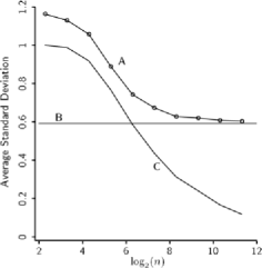
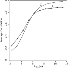
Simulation I: Illustrations of Proposition 5.1. In the first set of simulations we fixed $p=50$ and generated $\bolds{\Gamma}$ once at the outset, giving $\|\bolds{\Gamma}\|=8.2$. The diagonal elements of $\bolds{\Delta}$ were 50 regularly spaced values between 1 and 101. According to Corollary 5.2(i), as $n\rightarrow\infty$ the variance of $\widehat{{\mathbf{R}}}_{\mathbf{I}}-{\mathbf{R}}$ should converge to $\operatorname{var}(\bolds{\nu})=0.595^{2}$, where the value was determined by substituting the simulation parameters into (12). This conclusion is supported by the results in Figure 1(a), where we see that the standard deviation curve A converges nicely to the predicted asymptotic value marked by line segment B. Curve C in Figure 1(a) was generated by setting $\bolds{\Gamma}=(8.2,0,\ldots,0)^{T}$, so $\operatorname{span}(\bolds{\gamma})$ is now a reducing subspace of $\bolds{\rho}=\bolds{\Delta}$. In this case Corollary 5.2(ii) predicts that $\widehat{{\mathbf{R}}}_{\mathbf{I}}-{\mathbf{R}}$ will converge to 0 at the usual root-$n$ rate. That conclusion is supported by curve C. Curves A and C in Figure 1(b) correspond to those in Figure 1(a), except the average correlation is plotted on the vertical axis. Evidently the correlations for curve A are converging to a value close to 0.9, while those for curve C are converging to 1. Curve A suggests that when $\operatorname{var}(\bolds{\nu})>0$ we might still gain useful results in practice if the correlation is sufficiently large.

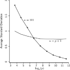
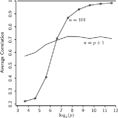
Simulation II: Bounded and unbounded error variances. The structure of the second set of simulations was like the first set, except we varied $n=p/2$ and, at the start of each replication, $\bolds{\Gamma}$ and $Y$ were generated anew and the diagonal elements of $\bolds{\Delta}$ were sampled from the uniform distribution on the interval $(1,u)$, where $u=101$ or $u=p+1$. The regeneration at the start of each replication was used to avoid tying results to a particular parameter configuration. For this simulation the ratio of the systematic variation in ${\mathbf{X}}$ to its total variation is $\operatorname{var}^{-1/2}({\mathbf{X}})\operatorname{var}(\mathrm{E}({\mathbf{X}}|\bolds{\Gamma},Y,\bolds{\Delta}))\operatorname{var}^{-1/2}({\mathbf{X}})=(2/(u+3))\mathbf{I}_{p}$, where the moments were computed over the simulation distributions of ${\mathbf{X}}$, $Y$, $\bolds{\Gamma}$ and $\bolds{\Delta}$. Consequently, it seems fair to characterize the signal as weak when $u\geq 101$, since then the systematic variation accounts for less than 2% of the total variation.

The regression is abundant and $\kappa=o(1)$ in this simulation. Additionally, when $u=101$, $\|\bolds{\rho}\|$ is bounded and the results of Corollary 5.1(i) apply, $\widehat{{\mathbf{R}}}_{\mathbf{I}}-{\mathbf{R}}=O_{p}(n^{-1/2})$. The simulation results for this case, which are shown by the curves labeled “$u=101$” in Figure 2, support the claim that standard deviation of

(a)	(b)

Figure 2: Results from simulation II described in Section 5.2 with $n=p/2$, ${\mathbf{W}}=\mathbf{I}_{p}$, $Y\sim N(0,1)$, $\bolds{\Gamma}\sim N(0,\mathbf{I}_{p})$ and $\operatorname{diag}(\bolds{\Delta})\sim\operatorname{Uniform}(1,u)$. (a) Standard deviation of $\widehat{{\mathbf{R}}}_{\mathbf{I}}-{\mathbf{R}}$; (b) correlation $(\widehat{{\mathbf{R}}}_{\mathbf{I}},{\mathbf{R}})$.

$\widehat{{\mathbf{R}}}_{\mathbf{I}}-{\mathbf{R}}$ is converging to 0 and the correlation between $\widehat{{\mathbf{R}}}_{\mathbf{I}}$ and ${\mathbf{R}}$ is approaching 1. On the other hand, when $u=p+1$, $\|\bolds{\rho}\|$ is unbounded and the results of Corollary 5.1 do not apply. However, we still might expect the standard deviation and correlation to converge to values away from 0 and 1. The simulation results shown by the curves labeled $u=p+1$ in Figure 2 sustain this expectation.

5.3 SPICE

Beginning with a little background, we turn in this section to weight matrices $\widehat{{\mathbf{W}}}\in{\mathbb{R}}^{p\times p}$ selected by using SPICE.

Restricting attention to population weight matrices that are equal to the inverse of the error covariance matrix, ${\mathbf{W}}=\bolds{\Delta}^{-1}$, allows for the application of some modern regularized inverse covariance estimators with reasonable convergence rates of $\widehat{{\mathbf{W}}}\in{\mathbb{R}}^{p\times p}$ as $n,p\rightarrow\infty$. For example, rates of convergence have been established for banding or tapering [Bickel and Levina (2008a)] and element-wise thresholding [Bickel and Levina (2008b)] of the sample covariance matrix. However, using these approaches to estimate the population weight matrix is problematic. Banding/tapering the sample covariance matrix is not invariant under permutations of variable labels, and in finite samples, both banding/tapering and thresholding the sample covariance matrix may produce an estimator of the covariance matrix that is not positive definite. To avoid these problems, we further restrict our attention to covariance estimators that are positive definite in finite samples and are invariant to permutations of variable labels. Several authors have recently analyzed the high-dimensional inverse covariance estimator formed through $L_{1}$-penalized likelihood optimization. We will use a particular version to estimate the population weight matrix (equivalently the inverse error covariance matrix) which was named SPICE by Rothman et al. (2008) for “sparse permutation invariant covariance estimator.”

Let $\tilde{n}=n-r-1$ and let

$$\widehat{\bolds{\Delta}}=\tilde{n}^{-1}{\mathbb{Z}}^{T}{\mathbf{Q}}_{\mathbb{F}}{\mathbb{Z}}\in{\mathbb{R}}^{p\times p}$$ (13)

denote the residual sample covariance matrix from the linear regression of ${\mathbf{X}}$ on ${\mathbf{f}}$. We construct $\widehat{{\mathbf{W}}}_{\lambda}=\widehat{\bolds{\Delta}}{}^{-1}_{\lambda}$ using

$$\widehat{\bolds{\Omega}}_{\lambda} \,{=}\, \mathop{\arg\min}_{{\bolds{\Omega}}>0}\biggl{[}\operatorname{tr}\{\operatorname{diag}^{-1/2}(\widehat{\bolds{\Delta}})\widehat{\bolds{\Delta}}\operatorname{diag}^{-1/2}(\widehat{\bolds{\Delta}})\bolds{\Omega}\}\!-\!{\log}|\bolds{\Omega}|\!+\!\lambda\sum_{i\neq j}|\Omega_{ij}|\biggr{]},$$

$$\widehat{\bolds{\Delta}}{}^{-1}_{\lambda} \,{=}\, \operatorname{diag}^{-1/2}(\widehat{\bolds{\Delta}})\widehat{\bolds{\Omega}}_{\lambda}\operatorname{diag}^{-1/2}(\widehat{\bolds{\Delta}}),$$

where $\lambda\geq 0$ is a tuning parameter and $\Omega_{ij}$ is the $(i,j)$ element of $\bolds{\Omega}$. The optimization in (5.3) produces a sparse estimator $\widehat{\bolds{\Omega}}_{\lambda}$ of the inverse error correlation matrix $\bolds{\Omega}$, which is then rescaled by the residual sample standard deviations to give the inverse error covariance estimator $\widehat{\bolds{\Delta}}{}^{-1}_{\lambda}$. The use of $L_{1}$-penalized likelihood optimization to estimate a sparse inverse covariance matrix has been studied extensively in the literature [d’Aspremont, Banerjee and El Ghaoui (2008), Yuan and Lin (2007), Friedman, Hastie and Tibshirani (2008), Rothman et al. (2008), Lam and Fan (2009)]. Although we impose sparsity on the off-diagonal entries of the inverse error covariance matrix $\bolds{\Delta}^{-1}$, we expect that in many situations $\bolds{\Delta}^{-1}$ may not be sparse. We selected this estimator since it is able to adapt, with its tuning parameter, to both sparse and less sparse estimates, and can lead to a substantial reduction in variability of our reduction estimator when $p$ is large; however, using small values of the tuning parameter $\lambda$ to give less-sparse inverse error covariance estimates leads to slow convergence of algorithms to solve (5.3) when $p$ is large.

Rothman et al. (2008) established the consistency of $\widehat{\bolds{\Delta}}{}^{-1}_{\lambda}$ in a special case of model (2) characterized by the following four conditions: (A) $r=0$, so $\widehat{\bolds{\Delta}}={\mathbb{Z}}^{T}{\mathbb{Z}}/\tilde{n}$ is the usual estimator of the marginal covariance matrix of ${\mathbf{X}}$. (B) The errors $\bolds{\varepsilon}$ are normally distributed with mean 0 and variance $\bolds{\Delta}$. (C) The largest $\varphi_{\max}(\bolds{\Delta})$ and smallest $\varphi_{\min}(\bolds{\Delta})$ eigenvalues of $\bolds{\Delta}$ are uniformly bounded; that is, for all $p$

$$0<\underline{k}\leq\varphi_{\min}(\bolds{\Delta})\leq\varphi_{\max}(\bolds{\Delta})\leq\overline{k}<\infty,$$ (15)

where $\underline{k}$ and $\overline{k}$ are constants. (D) $\lambda\asymp\sqrt{\frac{\log p}{n}}$. Then [Rothman et al. (2008)]

$$\|\widehat{\bolds{\Delta}}{}^{-1}_{\lambda}-\bolds{\Delta}^{-1}\|=O_{p}\bigl{(}\sqrt{n^{-1}\bigl{(}s(p)+1\bigr{)}\log p}\bigr{)},$$ (16)

where $s(p)$ is the total number of nonzero off-diagonal entries of $\bolds{\Delta}^{-1}$, which could grow with $p$.

In this application ${\mathbf{S}}={\mathbf{W}}^{-1/2}(\widehat{{\mathbf{W}}}-{\mathbf{W}}){\mathbf{W}}^{-1/2}=\bolds{\Delta}^{1/2}(\widehat{\bolds{\Delta}}{}^{-1}_{\lambda}-\bolds{\Delta}^{-1})\bolds{\Delta}^{1/2}$. To find the order of $\|{\mathbf{S}}\|$ and thereby allow application of Proposition 5.1 with SPICE, we relax the conditions of Rothman et al. (2008) by allowing (A^∗) $r>0$ and assuming that (B^∗) the elements $\varepsilon_{j}$ of $\bolds{\varepsilon}$ are uniformly sub-Gaussian random variables. That is, we assume there exist positive constants $K_{1}$ and $K_{2}$ such that for all $t>0$ and all $p$

$$P(|\varepsilon_{j}|>t)\leq K_{1}e^{-K_{2}t^{2}},\qquad j=1,\ldots,p.$$ (17)

This assumption is compatible with universal conditions (W.1) and (W.2). When the $\varepsilon_{j}$’s are normal, it is equivalent to requiring that their variances are uniformly bounded as $p\rightarrow\infty$. The following lemma gives the orders of $\|{\mathbf{S}}\|$ and $\|\mathrm{E}({\mathbf{S}}^{2})\|$ required for conditions (S.1) and (S.2).

Lemma 5.1

Let $\widehat{{\mathbf{W}}}=\widehat{\bolds{\Delta}}{}^{-1}_{\lambda}$, let $s\equiv s(p)$ be the total number of nonzero off-diagonal entries of $\bolds{\Delta}$ and let $\omega_{\mathrm{spice}}(n,p)=\sqrt{n^{-1}(s+1)\log p}$. Under conditions (B^∗), (C) and (D), $\|{\mathbf{S}}\|=O_{p}(\omega_{\mathrm{spice}})$ and $\|\mathrm{E}({\mathbf{S}}^{2})\|=O(\omega_{\mathrm{spice}}^{2})$.

Applying Proposition 5.1(iii) in the context of SPICE, $\bolds{\rho}=\mathbf{I}_{p}$ because ${\mathbf{W}}=\bolds{\Delta}^{-1}$. Consequently, $\operatorname{var}(\bolds{\nu})=0$ and $\psi=\sqrt{p}/h\sqrt{n}\leq\kappa$. From this we immediately get the following convergence rate bound for $\widehat{{\mathbf{R}}}_{{\widehat{\bolds{\Delta}}}_{\lambda}}\equiv\widehat{{\mathbf{R}}}_{\mathrm{spice}}$.

Proposition 5.2

Assume that the conditions and notation of Lemma 5.1 hold. Then

$$\widehat{{\mathbf{R}}}_{\mathrm{spice}}({\mathbf{X}}_{N})-{\mathbf{R}}({\mathbf{X}}_{N})=O_{p}(\kappa)+O_{p}(\omega_{\mathrm{spice}}).$$ (18)

If the number $s$ of nonzero off-diagonal entries of $\bolds{\Delta}^{-1}$ is bounded as $p\rightarrow\infty$ and the regression is abundant ($\kappa\asymp n^{-1/2}$), then $\widehat{{\mathbf{R}}}_{\mathrm{spice}}({\mathbf{X}}_{N})-{\mathbf{R}}({\mathbf{X}}_{N})=O_{p}(n^{-1/2}\log^{1/2}p)$. This allows for the number of variables $p$ to grow much faster than the sample size, so long as $s$ is bounded. On the other extreme, if there is no sparsity so that $s=p(p-1)$, then the bounding rate implied in Proposition 5.2 would seem to indicate that $n$ needs to be large relative to $\{p(p-1)+1\}\log p$ for good results. Based on our results for normal errors in Section 6, we anticipate that this rate is not sharp, most notably when $\bolds{\Delta}^{-1}$ is not sparse, and that it can be improved, particularly when additional structure is imposed (see Section 6).

Conditions (B^∗), (C) and (D) required for Proposition 5.2 are in addition to the active universal constraints stated in Section 4. Of the universal constraints, we still require the signal rate property (8), the order $\kappa=O(1)$ and (W.2). The remaining universal constraints are implied by the conditions of the proposition: since $\bolds{\rho}=\mathbf{I}_{p}$, the regression is stable by Lemma 4.1, (W.1) holds and $\psi\leq\kappa$ so (10) holds.

5.4 A diagonal weight matrix

We include in this section a discussion of the asymptotic behavior of the reduction based on the diagonal weight matrix $\widehat{{\mathbf{W}}}=\operatorname{diag}^{-1}(\widehat{\bolds{\Delta}})$, where $\widehat{\bolds{\Delta}}$ was defined in (13). This weight matrix, which corresponds to the population weight matrix ${\mathbf{W}}=\operatorname{diag}^{-1}(\bolds{\Delta})$, ignores the residual correlations and adjusts only for residual variances. However, in contrast to SPICE, there is no tuning parameter involved and so its computation is not an issue.

With ${\mathbf{W}}=\operatorname{diag}^{-1}(\bolds{\Delta})$, $\bolds{\rho}$ is the residual correlation matrix and

$${\mathbf{S}}=\operatorname{diag}^{1/2}(\bolds{\Delta})\bigl{(}\operatorname{diag}^{-1}(\widehat{\bolds{\Delta}})-\operatorname{diag}^{-1}(\bolds{\Delta})\bigr{)}\operatorname{diag}^{1/2}(\bolds{\Delta}).$$

The following lemma gives the orders of $\|{\mathbf{S}}\|$ and $\|\mathrm{E}({\mathbf{S}}^{2})\|$ in preparation for application of Proposition 5.1.

Lemma 5.2

Let $\widehat{{\mathbf{W}}}=\operatorname{diag}^{-1}(\widehat{\bolds{\Delta}})$, let $\omega_{\mathrm{diag}}=n^{-1/2}\log^{1/2}p$ and assume that the elements $\varepsilon_{j}$ of the errors $\bolds{\varepsilon}$ are sub-Gaussian random variables. Then $\|{\mathbf{S}}\|=O_{p}(\omega_{\mathrm{diag}})$ and $\|\mathrm{E}({\mathbf{S}}^{2})\|=O(\omega_{\mathrm{diag}}^{2})$.

In contrast to Lemma 5.1, here we require only that the errors are sub-Gaussian and not uniformly sub-Gaussian. This is because the diagonal weight matrix effectively standardizes the variances.

Proposition 5.3

Assume that the conditions and notation of Lemma 5.2 hold. Then

$$\widehat{{\mathbf{R}}}_{\mathrm{diag}}({\mathbf{X}}_{N})-{\mathbf{R}}({\mathbf{X}}_{N})=\bolds{\nu}+O_{p}(\kappa)+O_{p}(\psi)+O_{p}(\omega_{\mathrm{diag}}).$$ (19)

The order (19) for the diagonal weight matrix can be smaller than, equal to, or greater than the order (18) for the SPICE weight matrix, depending on the underlying structure of the regression. Using results from the discussion of Section 5.1, if $\|\bolds{\rho}\|=O(\sqrt{h})$ and $\operatorname{span}(\bolds{\gamma})$ is a reducing subspace of $\bolds{\rho}$, then $\widehat{{\mathbf{R}}}_{\mathrm{diag}}({\mathbf{X}}_{N})-{\mathbf{R}}({\mathbf{X}}_{N})=O_{p}(\kappa)+O_{p}(\omega_{\mathrm{diag}})$, and thus the diagonal weight matrix can produce a better rate because $\omega_{\mathrm{diag}}\leq\omega_{\mathrm{spice}}$. If $\bolds{\Delta}$ is itself a diagonal matrix, then $s=0$, $\operatorname{var}(\bolds{\nu})=0$, $\kappa\geq\psi$ and $\omega_{\mathrm{diag}}=\omega_{\mathrm{spice}}$, and consequently

$$\widehat{{\mathbf{R}}}_{\mathrm{diag}}({\mathbf{X}}_{N})-{\mathbf{R}}({\mathbf{X}}_{N})=O_{p}(\kappa)+O_{p}(\omega_{\mathrm{diag}}).$$ (20)

In this case the two weight matrices result in the same order, so there seems to be no asymptotic loss incurred by SPICE when $\bolds{\Delta}$ is diagonal.

6 Normal errors and $\xi=\beta{\mathbf{f}}$

We consider in this section the relatively ideal situation in which the errors $\bolds{\varepsilon}$ are normally distributed and the user-selected basis function ${\mathbf{f}}$ correctly models the true coordinates, so $\bolds{\xi}_{i}=\bolds{\beta}{\mathbf{f}}_{i}$, $i=1,\ldots,n$, for some fixed matrix $\bolds{\beta}\in{\mathbb{R}}^{d\times r}$ of rank $d$. The diagonal weight matrix is revisited under these assumptions in Section 6.1. In Section 6.2 we add the sample size constraint $n>p+r+4$ so $\widehat{\bolds{\Delta}}>0$. The importance of this setting is that we can obtain the oracle rate.

6.1 Diagonal weight matrix

The rates (20) for a diagonal $\bolds{\Delta}$ can be sharpened considerably when the errors are normal and $\bolds{\xi}=\bolds{\beta}{\mathbf{f}}$:

Proposition 6.1

Assume that $\bolds{\varepsilon}\sim N(0,\bolds{\Delta})$, $\bolds{\Delta}$ is a diagonal matrix, $\bolds{\xi}=\bolds{\beta}{\mathbf{f}}$, $n>r+5$ and $\widehat{{\mathbf{W}}}=\operatorname{diag}^{-1}(\widehat{\bolds{\Delta}})$. Then $\widehat{{\mathbf{R}}}_{\mathrm{diag}}({\mathbf{X}}_{N})-{\mathbf{R}}({\mathbf{X}}_{N})=O_{p}(\kappa)$.

We see from this proposition that when the errors are normal, the order $O_{p}(\omega_{\mathrm{diag}})$ that appears in (20) is no longer present and the rate for $\widehat{{\mathbf{R}}}_{\mathrm{diag}}$ reduces to the oracle rate $\kappa^{-1}$. The condition $n>r+5$ stated in Proposition 6.1 is needed to insure the existence of the variance of an inverse chi-squared random variable. Its proof is omitted from the supplement since it follows the same lines as the proof of Proposition 5.1.

6.2 $n>p+r+4$

Recalling that $\widehat{\bolds{\Delta}}\in{\mathbb{R}}^{p\times p}$ is the residual covariance matrix defined in (13), this constraint on $n$ means that $\widehat{\bolds{\Delta}}>0$ with probability 1, allowing the straightforward use of $\widehat{{\mathbf{W}}}=\widehat{\bolds{\Delta}}^{-1}$ as the weight matrix. The population weight matrix is ${\mathbf{W}}=\bolds{\Delta}^{-1}$ with corresponding ${\mathbf{S}}=\bolds{\Delta}^{1/2}\widehat{\bolds{\Delta}}{}^{-1}\bolds{\Delta}^{1/2}-\mathbf{I}_{p}$. The asymptotic behavior of $\|{\mathbf{S}}\|$ in this setting can be obtained as follows: phrased in the context of this article, suppose that $r=0$ so $\widehat{\bolds{\Delta}}=(n-1)^{-1}\sum_{i=1}^{n}({\mathbf{X}}_{i}-\bar{{\mathbf{X}}})({\mathbf{X}}_{i}-\bar{{\mathbf{X}}})^{T}$. Johnstone (2001) [see also Bai (1999), page 635] showed that $\varphi_{\max}(\bolds{\Delta}^{-1/2}\widehat{\bolds{\Delta}}\bolds{\Delta}^{-1/2})-1\asymp_{p}(\sqrt{p/n})$ and Paul (2005) showed that $\varphi_{\min}(\bolds{\Delta}^{-1/2}\widehat{\bolds{\Delta}}\bolds{\Delta}^{-1/2})-1\asymp_{p}(\sqrt{p/n})$ when $p/n\rightarrow a~{}\in[0,1)$. Together these results imply that $\|{\mathbf{S}}\|\asymp_{p}(\sqrt{p/n})$ and therefore $\|{\mathbf{S}}\|\rightarrow 0$ in probability if and only if $p/n\rightarrow 0$, which gives the order for condition (S.1). Still with $r=0$, since $(n-1)\widehat{\bolds{\Delta}}{}^{-1}$ is distributed as the inverse of a Wishart $W_{p}(\bolds{\Delta},n-1)$ matrix, we used results from von Rosen (1988) to verify condition (S.2). Combining these results with Proposition 5.1 we have

$$\widehat{{\mathbf{R}}}_{\widehat{{\bolds{\Delta}}}}({\mathbf{X}}_{N})-{\mathbf{R}}({\mathbf{X}}_{N})=O_{p}\bigl{(}\sqrt{p/n}\bigr{)},$$ (21)

where $\widehat{{\mathbf{R}}}_{\widehat{{\bolds{\Delta}}}}$ denotes the reduction with $\widehat{{\mathbf{W}}}=\widehat{\bolds{\Delta}}{}^{-1}$. This suggests that it may be reasonable to use $\widehat{\bolds{\Delta}}{}^{-1}$ as the weight matrix only when $n$ is large relative to $p$, essentially sending us back to the usual requirement. In the next proposition we show this is not the case with $r>0$ because the order in (21) is in fact too large.

Proposition 6.2

Assume that $\bolds{\varepsilon}\sim N_{p}(0,\bolds{\Delta})$, $\bolds{\xi}=\bolds{\beta}{\mathbf{f}}$, $n>p+r+4$ and $p/n\rightarrow[0,1)$. Let $a~{}=(n-p-1)^{-1}$. Then when $\widehat{{\mathbf{W}}}=\widehat{\bolds{\Delta}}{}^{-1}$:

$h^{-1}\mathrm{E}(\widehat{\mathbf{K}})=a(n-r-1)\{\mathbf{K}+\kappa^{2}\mathbf{I}_{r}\},$

$h^{-1}(p)\{\widehat{\mathbf{K}}-\mathrm{E}(\widehat{\mathbf{K}})\}=O_{p}(1/\sqrt{n})$,

$\widehat{{\mathbf{R}}}_{\widehat{{\bolds{\Delta}}}}({\mathbf{X}}_{N})-{\mathbf{R}}({\mathbf{X}}_{N})=O_{p}(\kappa)$.

Recall from Corollary 5.1 that when $\widehat{{\mathbf{W}}}=\bolds{\Delta}^{-1}$, we obtain the oracle rate $\widehat{{\mathbf{R}}}_{{\bolds{\Delta}}}({\mathbf{X}}_{N})-{\mathbf{R}}({\mathbf{X}}_{N})=O_{p}(\kappa)$. Comparing this result with the conclusion of Proposition 6.2(iii), we see that there is no impact on the rate of convergence when using $\widehat{{\mathbf{W}}}=\widehat{\bolds{\Delta}}{}^{-1}$ instead of $\widehat{{\mathbf{W}}}=\bolds{\Delta}^{-1}$, both weight matrices giving estimators that converge at the oracle rate. In contrast to the gross bound given in (21), Proposition 6.2 indicates that it may in fact be quite reasonable to use $\widehat{\bolds{\Delta}}{}^{-1}$ as the weight matrix when $n>p+r+4$, without requiring $n$ to be large relative to $p$.

Properties of the normal and the accurate modeling of $\bolds{\xi}=\bolds{\beta}{\mathbf{f}}$ surely contribute to the oracle rate of Proposition 6.2. Recall from (5) that $\widehat{\mathbf{K}}=\bolds{\Phi}_{n}^{1/2}\widehat{{\mathbf{B}}}^{T}\widehat{{\mathbf{W}}}\widehat{{\mathbf{B}}}\bolds{\Phi}_{n}^{1/2}$. Under the conditions of Proposition 6.2, $\widehat{{\mathbf{B}}}\perp\perp\widehat{{\mathbf{W}}}$, which is not required for our most general results given in Proposition 5.1. Additionally, we were able to use exact calculations in places where bounding was otherwise employed. The inverse residual sum of squares matrix $(n-r-1)\widehat{\bolds{\Delta}}{}^{-1}$ is distributed as the inverse of a Wishart $W_{p}(\bolds{\Delta},n-r-1)$ matrix and the moments of an inverse Wishart derived by von Rosen (1988) were used extensively in the proof of Proposition 6.2. For instance, although $\widehat{\bolds{\Delta}}$ has an inverse with probability 1 when $n>p+r+1$, the constraint on $n$ in the hypothesis is needed to ensure the existence of the variance of the inverse Wishart.

The signal rate (8) and the order $\kappa=O(1)$ are still required for Proposition 6.2, but its hypothesis implies all the other universal conditions stated in Section 4: since ${\mathbf{W}}=\bolds{\Delta}^{-1}$ we have $\bolds{\rho}=\mathbf{I}_{p}$ and thus (1) the regression is stable by Lemma 4.1, (2) $\psi\leq\kappa$ so (10) holds, (3) $\mathrm{E}(\bolds{\varepsilon}^{T}{\mathbf{W}}\bolds{\varepsilon})=p$ so condition (W.1) holds, and (4) condition (W.2) holds by Lemma 4.2(i).

7 Simulations

The effects of predictor correlations are often a concern when dealing with high-dimensional regressions. In this section, we introduce predictor correlations into our simulations to give some intuition about their impact on the four reduction estimators.

The computation of the four reduction estimators $\widehat{{\mathbf{R}}}_{\mathbf{I}},\widehat{{\mathbf{R}}}_{\mathrm{spice}},\widehat{{\mathbf{R}}}_{\mathrm{diag}}$ and $\widehat{{\mathbf{R}}}_{\widehat{{\bolds{\Delta}}}}$ relies on the computation of their weight matrix estimators $\widehat{{\mathbf{W}}}$, which are available in closed form for $\widehat{{\mathbf{R}}}_{\mathbf{I}},\widehat{{\mathbf{R}}}_{\mathrm{diag}}$ and $\widehat{{\mathbf{R}}}_{\widehat{{\bolds{\Delta}}}}$; however, computing the weight matrix estimator for $\widehat{{\mathbf{R}}}_{\mathrm{spice}}$ requires us to select its tuning parameter $\lambda$ and to use an iterative algorithm.

7.1 Computation and tuning parameter selection for $\widehat{{\mathbf{R}}}_{\mathrm{spice}}$

Several computational algorithms [d’Aspremont, Banerjee and El Ghaoui (2008), Yuan and Lin (2007), Friedman, Hastie and Tibshirani (2008), Rothman et al. (2008)] have been proposed to compute the solution to (5.3), of which we propose to use the graphical lasso (glasso) algorithm of Friedman, Hastie and Tibshirani (2008). We employ $K$-fold cross-validation to select the tuning parameter $\lambda$ for the weight matrix estimator $\widehat{{\mathbf{W}}}_{\lambda}\equiv\widehat{\bolds{\Delta}}{}^{-1}_{\lambda}$, where we minimize the validation negative log-likelihood. Specifically, we solve $\widehat{\lambda}=\arg\min_{\lambda}\sum_{k=1}^{K}g_{k}(\lambda)$ where

$$g_{k}(\lambda) = \operatorname{tr}\bigl{[}n_{k}^{-1}{\mathbf{A}}_{(k,\lambda)}^{T}{\mathbf{A}}_{(k,\lambda)}\widehat{{\mathbf{W}}}_{\lambda}^{(-k)}\bigr{]}-{\log}\bigl{|}\widehat{{\mathbf{W}}}_{\lambda}^{(-k)}\bigr{|},$$

$${\mathbf{A}}_{(k,\lambda)} = {{\mathbb{Z}}}^{(k)}-{\mathbb{F}}^{(k)}\widehat{\mathbf{b}}^{(-k)T}_{\lambda}\widehat{\bolds{\Gamma}}{}^{(-k)T}_{\lambda}.$$

In the above expression, a superscript of $(k)$ indicates that the quantity is based on the observations inside the $k$th fold, and a superscript of $(-k)$ indicates that the quantity is based on observations outside of the $k$th fold, and $n_{k}$ is the number of observations in the $k$th fold.

7.2 Simulation settings

The simulated data were generated from ${\mathbf{X}}_{i}=\bolds{\Gamma}\bolds{\xi}_{i}+\bolds{\varepsilon}_{i}$, $i=1,\ldots,n$, where $Y_{1},\ldots,Y_{n}$ is a sequence of independent random variables, $\bolds{\varepsilon}_{1},\ldots,\bolds{\varepsilon}_{n}$ are independent copies of $\bolds{\varepsilon}$, a $p$-variate normal random vector with mean 0 and variance $\bolds{\Delta}$, and $\bolds{\xi}_{i}=\bolds{\xi}(Y_{i})$ is specified later. As in the second simulation of Section 5.2, $\bolds{\Gamma}$ and $\bolds{\Delta}$ were produced anew at the start of each replication, with the elements of $\bolds{\Gamma}\in{\mathbb{R}}^{p}$ always generated as a sequence of independent standard normal variables and $\bolds{\Delta}$ generated as $\mathbf{D}^{1/2}\bolds{\Theta}\mathbf{D}^{1/2}$ where $\mathbf{D}$ is a diagonal matrix with diagonal elements sampled from a uniform $(1,101)$ distribution and $\bolds{\Theta}=(\theta_{ij})$ is a correlation matrix with exponentially decreasing correlations, $\theta_{ij}=\theta^{|i-j|}$ with parameter $0<\theta<1$. This structure has been used frequently to assess the impact of predictor correlations on high-dimensional methodology [see, e.g., Bickel and Levina (2008b), Li and Yin (2008)]. For all four reduction estimators, $h\asymp p$ implying $\kappa=n^{-1/2}$.

For each replication, we determined $\widehat{{\mathbf{R}}}({\mathbf{X}}_{N,j})$ and ${\mathbf{R}}({\mathbf{X}}_{N,j})$ at $j=1,\ldots,100$ new data points generated from the original model. We assess performance by computing the magnitude of the sample correlation between $\widehat{{\mathbf{R}}}$ and ${\mathbf{R}}$ over the 100 new data points. The results are based on 200 independent replications.

For a given weight matrix ${\mathbf{W}}$, the expected signal strength over simulation replications is determined by $\mathrm{E}_{\mathrm{sim}}(\bolds{\Gamma}^{T}{\mathbf{W}}\bolds{\Gamma})=\mathrm{E}_{\mathrm{sim}}\operatorname{tr}({\mathbf{W}})$, where $\mathrm{E}_{\mathrm{sim}}$ denotes expectation over the simulations. For ${\mathbf{W}}=\operatorname{diag}^{-1}(\bolds{\Delta})$, $\mathrm{E}_{\mathrm{sim}}[\operatorname{tr}({\mathbf{W}})]=\log(101)/100$, but for ${\mathbf{W}}=\bolds{\Delta}^{-1}$,

$$\mathrm{E}_{\mathrm{sim}}[\operatorname{tr}({\mathbf{W}})]=\operatorname{tr}(\bolds{\Theta}^{-1})\log(101)/100=\frac{2+(p-2)(1+\theta^{2})}{1-\theta^{2}}\frac{\log 101}{100}.$$

From this we see that the expected signal strength increases with $\theta$ when using $\widehat{{\mathbf{R}}}_{\widehat{{\bolds{\Delta}}}}$ and $\widehat{{\mathbf{R}}}_{\mathrm{spice}}$, but is constant in $\theta$ when using $\widehat{{\mathbf{R}}}_{\mathrm{diag}}$ and $\widehat{{\mathbf{R}}}_{\mathbf{I}}$. In addition, $\|\bolds{\Delta}\|=O(1)$ since $\|\bolds{\Delta}\|\leq\|\bolds{\Delta}\|_{\infty}=\max_{j}\sum_{i}\delta_{ij}\leq 2\cdot 101/(1-\theta)$, where $\delta_{ij}$ is element $(i,j)$ of $\bolds{\Delta}$.

With this general setup we next report results for various combinations of $n$, $p$, $\bolds{\xi}$ and ${\mathbf{f}}$. We extended the applicability of $\widehat{{\mathbf{R}}}_{\widehat{{\bolds{\Delta}}}}$ to regressions in which $n<p$ by using the Moore–Penrose generalized inverse of $\widehat{\bolds{\Delta}}$, although we have presented no asymptotic results for this case.

7.3 Correctly specified $\xi=\beta{\mathbf{f}}$

In this section we consider a simple case where $\bolds{\xi}=Y$, giving $d=1$, and ${\mathbf{f}}=(Y,Y^{2},Y^{3},Y^{4})$, so $r=4$ and $\bolds{\xi}=\bolds{\beta}{\mathbf{f}}$, where $\bolds{\beta}=(1,0,0,0)$ and $Y$ was generated as a standard normal variate.

7.3.1 $n=p/2$ and $p\rightarrow\infty$

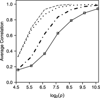
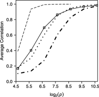
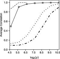
In this setting, $n$ and $p$ grow with $n=p/2$. For the reduction estimators $\widehat{{\mathbf{R}}}_{\mathbf{I}}$ and $\widehat{{\mathbf{R}}}_{\mathrm{diag}}$, $\|\bolds{\rho}\|=O(1)$, $\|\bolds{\rho}\|_{F}\leq\sqrt{p}\|\bolds{\rho}\|=O(\sqrt{p})$ which imply that $\psi=\kappa=n^{-1/2}$. Also, $\operatorname{var}(\bolds{\nu})\leq{\mathbf{G}}_{h}^{-1}\|\bolds{\Delta}\|/h=O(p^{-1})$, hence $\bolds{\nu}=O_{p}(p^{-1})$. Thus in this setting with $n\asymp p$, $\widehat{{\mathbf{R}}}_{\mathbf{I}}$ is $\sqrt{n}$-consistent and $\widehat{{\mathbf{R}}}_{\mathrm{diag}}$ is at least $\sqrt{n/\log n}$-consistent as $n,p\rightarrow\infty$.

Although $\|\bolds{\Delta}\|=O(1)$ and $\bolds{\Delta}^{-1}$ is a tri-diagonal matrix, our theoretical bounds for $\widehat{{\mathbf{R}}}_{\mathrm{spice}}$ guarantee consistency for this model only when $p$ is bounded and $n\rightarrow\infty$; however, a result established by Ravikumar et al. (2011), which requires additional assumptions, indicates that the weight matrix estimator for $\widehat{{\mathbf{R}}}_{\mathrm{spice}}$ is consistent when $\bolds{\Delta}^{-1}$ is tri-diagonal.

(a)	(b)
(c)

Figure 3: Comparison of the four estimators of ${\mathbf{R}}$: $\widehat{{\mathbf{R}}}_{\mathrm{spice}}$ (dashes), $\widehat{{\mathbf{R}}}_{\widehat{{\bolds{\Delta}}}}$ (solid), $\widehat{{\mathbf{R}}}_{\mathrm{diag}}$ (dots) and $\widehat{{\mathbf{R}}}_{\mathbf{I}}$ (dash dot), with exponential error correlations and $n=p/2$. Here (a) $\theta_{ij}=0.5^{|i-j|}$; (b) $\theta_{ij}=0.9^{|i-j|}$; (c) $\theta_{ij}=0.99^{|i-j|}$.

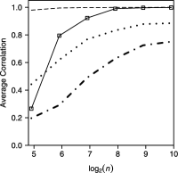
The results for $p$ and $n$ growing with $n=p/2$ are shown in Figure 3(a)–(c). All reduction estimators appear to be converging to the population reduction as $n,p\rightarrow\infty$, even though consistency is not guaranteed in this setting for $\widehat{{\mathbf{R}}}_{\mathrm{spice}}$ and $\widehat{{\mathbf{R}}}_{\widehat{{\bolds{\Delta}}}}$,

(a)	(b)
(c)

Figure 4: Comparison of the four estimators of ${\mathbf{R}}$: $\widehat{{\mathbf{R}}}_{\mathrm{spice}}$ (dashes), $\widehat{{\mathbf{R}}}_{\widehat{{\bolds{\Delta}}}}$ (solid), $\widehat{{\mathbf{R}}}_{\mathrm{diag}}$ (dots) and $\widehat{{\mathbf{R}}}_{\mathbf{I}}$ (dash dot), with exponential error correlations and $p=100$. Here (a) $\theta_{ij}=0.5^{|i-j|}$; (b) $\theta_{ij}=0.9^{|i-j|}$; (c) $\theta_{ij}=0.99^{|i-j|}$.

which uses a Moore–Penrose generalized inverse of the residual sample covariance matrix. Interestingly, when $p>n$, $\widehat{{\mathbf{R}}}_{\widehat{{\bolds{\Delta}}}}$ outperforms $\widehat{{\mathbf{R}}}_{\mathrm{diag}}$ and $\widehat{{\mathbf{R}}}_{\mathbf{I}}$ when $\theta\geq 0.9$. Results for $\widehat{{\mathbf{R}}}_{\mathrm{spice}}$ were computed up to $p=400$ when $\theta\leq 0.9$ and up to $p=100$ when $\theta=0.99$ due to intractable computation time required for the glasso algorithm. In scenarios when $\widehat{{\mathbf{R}}}_{\mathrm{spice}}$ was computed, it outperformed the other reduction estimators, particularly when $\theta=0.9$. As expected, larger values of $\theta$ lead to favorable performance for the reduction estimators with population weight matrix ${\mathbf{W}}=\bolds{\Delta}^{-1}$.

7.3.2 $p=100$ and $n\rightarrow\infty$

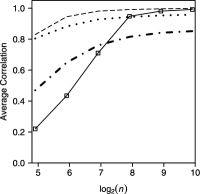
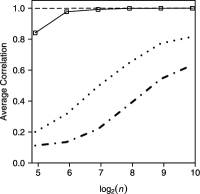
In this setting we fix $p=100$ and let $n$ grow. Our theory guarantees that $\widehat{{\mathbf{R}}}_{\mathrm{spice}}$ and $\widehat{{\mathbf{R}}}_{\widehat{{\bolds{\Delta}}}}$ are both $\sqrt{n}$-consistent. On the other hand, $\widehat{{\mathbf{R}}}_{\mathbf{I}}$ and $\widehat{{\mathbf{R}}}_{\mathrm{diag}}$ are inconsistent since $\operatorname{span}(\bolds{\gamma})$ is not a reducing subspace of $\bolds{\rho}$ and $p$ is bounded, implying $\bolds{\nu}$ fails to vanish.

The results for $p=100$ and $n$ growing are illustrated in Figure 4(a)–(c). As our theory suggests, the reduction estimators $\widehat{{\mathbf{R}}}_{\mathrm{spice}}$ and $\widehat{{\mathbf{R}}}_{\widehat{{\bolds{\Delta}}}}$ appear to be converging to the population reduction as $n$ increases. We see that $\widehat{{\mathbf{R}}}_{\mathrm{spice}}$ outperformed the other reduction estimators, particularly for relativelysmall $n$ when $\theta=0.9$. As expected, $\widehat{{\mathbf{R}}}_{\widehat{{\bolds{\Delta}}}}$ outperforms $\widehat{{\mathbf{R}}}_{\mathrm{diag}}$ and $\widehat{{\mathbf{R}}}_{\mathbf{I}}$ when $n$ is much larger than $p$ or when $\theta$ is large.

7.4 Results for $\xi\neq\beta{\mathbf{f}}$

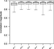
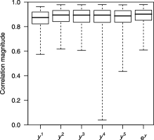
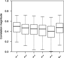
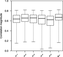
In this section we present results for a misspecified $\bolds{\xi}$ using $\bolds{\xi}=\operatorname{var}^{-1/2}(\exp(Y))[\exp(Y)-\mathrm{E}(\exp(Y))]$ where $Y\sim\operatorname{Unif}(0,4)$. Holding $n=50$ and $p=100$, we varied ${\mathbf{f}}=(y,y^{2},\ldots,y^{k})^{T}$ for $k=1,\ldots,5$ and ${\mathbf{f}}=\exp(y)$. The results are summarized in Figure 5 as

(a)	(b)
(c)	(d)

Figure 5: Estimators of ${\mathbf{R}}$ when ${\mathbf{f}}$ is misspecified, using exponential error correlations: $\theta_{ij}=0.5^{|i-j|}$, $n=50$ and $p=100$. Boxplots are labeled by the highest order term in ${\mathbf{f}}$. Here (a) $\widehat{{\mathbf{R}}}_{\mathrm{spice}}$; (b) $\widehat{{\mathbf{R}}}_{\mathrm{diag}}$; (c) $\widehat{{\mathbf{R}}}_{\widehat{{\bolds{\Delta}}}}$; (d) $\widehat{{\mathbf{R}}}_{\mathbf{I}}$.

boxplots of the correlation magnitudes over the 200 replications. Most striking is how little the choice of ${\mathbf{f}}$ seems to affect the estimators. This is likely because there are fairly strong correlations between $\bolds{\xi}$ and its approximations provided by the six ${\mathbf{f}}$’s used in the simulation, which satisfies condition (7). The relationship between the estimators are similar to those in Figure 4 at $n=50$, regardless of the choice of ${\mathbf{f}}$.

8 Spectroscopy application

To illustrate operation of the proposed methodology, we examine data from the potential application area mentioned in the Introduction. The response variable is the percentage of fat in samples of beef or pork, and the predictors are the absorbance spectra ($\log(1/R)$) from near-infrared transmittance for fat measured at every second wavelength between 850 and 1050 nm, giving $p=100$ with $n=54$ [Sæbø et al. (2007)]. The goal of the study is to predict the response from the absorbance spectra of a new sample. Our predictive framework is described in the next section. We return to the spectroscopy application in Section 8.2.

8.1 Prediction

We predict an unobserved response $Y_{N}$ associated with a new observed vector of predictors ${\mathbf{X}}_{N}$ by using the forward regression mean function: $Y_{\mathrm{pred}}=\mathrm{E}\{Y|{\mathbf{X}}_{N}\}=\mathrm{E}\{Y|{\mathbf{R}}({\mathbf{X}}_{N})\}$. However, the reduction ${\mathbf{R}}({\mathbf{X}})$ was based on the inverse regression ${\mathbf{X}}|Y$ and the development did not produce a direct estimator of $\mathrm{E}\{Y|{\mathbf{R}}({\mathbf{X}}_{N})\}$. There are perhaps several ways of using an estimated reduction for predicting a new response. Some authors have used standard data-analytic methods to develop predictive models based on $Y$ and the estimated reduction, and there are a variety of nonparametric regression methods that could also be used as well. We follow Adragni and Cook (2009) and use a kernel-type estimator of $\mathrm{E}\{Y|{\mathbf{R}}({\mathbf{X}}_{N})\}$ based on the relationship $\mathrm{E}\{Y|{\mathbf{X}}\,{=}\,{\mathbf{x}}\}\,{=}\,\mathrm{E}\{Y|{\mathbf{R}}({\mathbf{x}})\}\,{=}\,\mathrm{E}\{Yg({\mathbf{R}}({\mathbf{x}})|Y)\}/\mathrm{E}\{g({\mathbf{R}}({\mathbf{x}})|Y)\},$ where $g$ is the conditional density of ${\mathbf{R}}|Y$. This provides a method to estimate $\mathrm{E}\{Y|{\mathbf{X}}\}$:

$$\widehat{\mathrm{E}}\{Y|{\mathbf{X}}={\mathbf{x}}\} = \sum_{i=1}^{n}w_{i}({\mathbf{x}})Y_{i},$$

$$w_{i}({\mathbf{x}}) = \frac{\widehat{g}(\widehat{{\mathbf{R}}}({\mathbf{x}})|Y_{i})}{\sum_{i=1}^{n}\widehat{g}(\widehat{{\mathbf{R}}}({\mathbf{x}})|Y_{i})},$$

where $\widehat{g}$ denotes an estimate of the density and $\widehat{{\mathbf{R}}}$ is the estimated reduction. This estimator is reminiscent of a nonparametric kernel estimator, but there are consequential differences. The weights in a kernel estimator do not depend on the response, while the weights $w_{i}$ here do. Kernel weights typically depend on the full vector of predictors ${\mathbf{X}}$, while the weights here depend on ${\mathbf{X}}$ only through the estimated reduction $\widehat{{\mathbf{R}}}({\mathbf{x}})$. Multivariate kernels are usually taken to be the product of univariate kernels, corresponding here to treating the components of ${\mathbf{R}}$ as independent. Finally, there is no need for bandwidth estimation because the weights are determined entirely from $\widehat{g}$.

When $d$ is small relative to $p$ it may often be reasonable to assume that ${\mathbf{R}}({\mathbf{X}})|Y$ is normally distributed, which seems appropriate for the spectroscopy data. Ignoring constants not depending on $i$, we have

$$g({\mathbf{R}}({\mathbf{x}})|Y_{i})\propto\exp\bigl{\{}-(1/2)\bigl{(}{\mathbf{R}}({\mathbf{x}})-\bolds{\xi}_{i}\bigr{)}^{T}(\bolds{\Gamma}^{T}\bolds{\Delta}^{-1}\bolds{\Gamma})\bigl{(}{\mathbf{R}}({\mathbf{x}})-\bolds{\xi}_{i}\bigr{)}\bigr{\}}.$$

Substituting the estimators $\widehat{\bolds{\Gamma}}$, $\widehat{\mathbf{b}}{\mathbf{f}}_{i}$ and $\widehat{{\mathbf{W}}}$ for $\bolds{\Gamma}$, $\bolds{\xi}_{i}$ and $\bolds{\Delta}^{-1}$ gives the weights required for (8.1). For $\widehat{{\mathbf{R}}}_{\mathbf{I}}$, we set $\widehat{{\mathbf{W}}}=(p/\operatorname{tr}(\widehat{\bolds{\Delta}}))\mathbf{I}_{p}$.

(a)	(b)

Figure 6: Inverse response plot of the absorbance at wavelength 854 versus $Y$ for (a) pork samples and (b) pork and beef samples. The line for the pork sample is a fitted cubic polynomial. For pork and beef the lines represent a second-order polynomial fit to the data with one intercept for pork (solid) and a second intercept for beef (dashes).

8.2 Spectroscopy

Since there are only $p=100$ predictors it was straightforward, albeit somewhat tedious, to inspect inverse response plots of $X_{j}$ versus $Y$, $j=1,\ldots,100$, to gain information about the likely structure of ${\mathbf{f}}$. We performed two analyses; the first consisted of 54 pork samples and the second consisted of 103 meat samples of beef and pork. For a specified value of $d$, we assessed the fitted model by using the residual mean square $\mathrm{RMS}(d,r,\widehat{{\mathbf{R}}}_{(\cdot)})=\sum_{i=1}^{n}(Y_{i}-\widehat{Y}_{i})^{2}/n$, where the fitted values $\widehat{Y}_{i}=\widehat{\mathrm{E}}(Y|{\mathbf{X}}={\mathbf{X}}_{i})$ were determined using (8.1) with the indicated combination of $d$, $r$ and reduction $\widehat{{\mathbf{R}}}_{(\cdot)}$.

We selected the value of $d$ by adapting the permutation scenario developed by Cook and Yin (2001). The hypothesis $d=d_{0}$ was tested sequentially, starting at $d_{0}=0$ and estimating $d$ as the first hypothesized value that was not rejected. The test statistic $\mathrm{RMS}(d_{0}+1,r,{\mathbf{R}}_{(\cdot)})$ was compared to the distribution of $\mathrm{RMS}(d_{0}+1,r,{\mathbf{R}}_{(\cdot)})$ induced by $1000$ random permutations $\mathbf{J}$ applied to the rows of the predictor matrix $\mathbb{X}$ as follows:

$$\mathbb{X}_{\mathrm{perm}}=\mathbb{X}{\mathbf{P}}_{\widehat{\bolds{\Gamma}}(\widehat{{\mathbf{W}}})}^{T}+\mathbf{J}\mathbb{X}{\mathbf{Q}}_{\widehat{\bolds{\Gamma}}(\widehat{{\mathbf{W}}})}^{T},\vspace*{-3pt}$$

where $\widehat{\bolds{\Gamma}}$ and $\widehat{{\mathbf{W}}}$ were computed under the null hypothesis. This scheme leaves the signal $\mathbb{X}{\mathbf{P}}_{\widehat{\bolds{\Gamma}}(\widehat{{\mathbf{W}}})}^{T}$ intact while permuting the uninformative part of the predictors $\mathbb{X}{\mathbf{Q}}_{\widehat{\bolds{\Gamma}}(\widehat{{\mathbf{W}}})}^{T}$.

The multicollinearity of the predictors made computing the weight matrix estimator for $\widehat{{\mathbf{R}}}_{\mathrm{spice}}$ difficult for small values of its tuning parameter, values for which our cross-validation procedure recommended. We subsequently set its tuning parameter to $\lambda=2^{-10}$ for both analyses, since this was the smallest value for which a numerically stable solution was available.

8.2.1 Analysis of pork samples

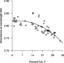
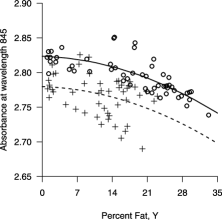
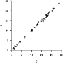
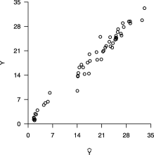
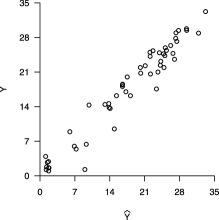
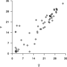
In this case we concluded that a cubic polynomial ${\mathbf{f}}(y)=(y,y^{2},y^{3})^{T}$ would be adequate; a representative plot is shown in Figure 6(a). Performing the permutation test to select $d$, the test statistic for $d=0$ using $\widehat{{\mathbf{R}}}_{\widehat{{\bolds{\Delta}}}}$ was $\mathrm{RMS}(1,3,\widehat{{\mathbf{R}}}_{\widehat{{\bolds{\Delta}}}})=0.31$ which was smaller than the smallest value $10.7$ of $\mathrm{RMS}(1,3,\widehat{{\mathbf{R}}}_{\widehat{{\bolds{\Delta}}}})$ observed among the $1000$ random permutations under the hypothesis that $d=0$. Since the test statistic is much smaller than can be accounted for by chance under the null hypothesis, we concluded that $d\geq 1$. Similarly, to test $d=1$, we observed $\mathrm{RMS}(2,3,\widehat{{\mathbf{R}}}_{\widehat{{\bolds{\Delta}}}})=0.29$ which fell at the 80th quantile of the permutation distribution of $\mathrm{RMS}(2,3,\widehat{{\mathbf{R}}}_{\widehat{{\bolds{\Delta}}}})$ under the hypothesis. Consequently, we used $d=1$ for the model. Comparisons with other values of $r$ figured in our choice $r=3$. Cross-validation using $\mathrm{RMS}$ as the criterion might also be used to select $d$.

(a)	(b)
(c)	(d)

Figure 7: Plots of the response versus fitted values for the four estimators (a) $\widehat{{\mathbf{R}}}_{\widehat{{\bolds{\Delta}}}}$, (b) $\widehat{{\mathbf{R}}}_{\mathrm{spice}}$, (c) $\widehat{{\mathbf{R}}}_{\mathrm{diag}}$ and (d) $\widehat{{\mathbf{R}}}_{\mathbf{I}}$, using the pork samples.

Fitting each of the four estimators with $d=1$, we found that $\mathrm{RMS}(1,3,\allowbreak\widehat{{\mathbf{R}}})=21.55$, $5.15$, $0.31$ and $2.15$ for $\widehat{{\mathbf{R}}}=\widehat{{\mathbf{R}}}_{\mathbf{I}}$, $\widehat{{\mathbf{R}}}_{\mathrm{diag}}$, $\widehat{{\mathbf{R}}}_{\widehat{{\bolds{\Delta}}}}$ and $\widehat{{\mathbf{R}}}_{\mathrm{spice}}$. Plots of $Y$ versus $\widehat{Y}$ are shown in Figure 7(a)–(d). The predictors in this illustration are highly collinear, as is typical in spectral data, and the relative performance of the four estimators is qualitatively similar to that shown in previous simulations; however, numerical instability degraded the performance of $\widehat{{\mathbf{R}}}_{\mathrm{spice}}$. The relative signal rates for the four estimators are reflected by the values of $\widehat{\bolds{\Gamma}}{}^{T}\widehat{{\mathbf{W}}}\widehat{\bolds{\Gamma}}=35.3$, $128.4$, $169.7$ and $63.38$ for $\widehat{{\mathbf{W}}}=(p/\operatorname{tr}(\widehat{\bolds{\Delta}}))\mathbf{I}_{d}$, $\operatorname{diag}^{-1}(\widehat{\bolds{\Delta}})$, $\widehat{\bolds{\Delta}}{}^{-}$ and $\widehat{\bolds{\Delta}}{}^{-1}_{\widehat{\lambda}}$.

8.2.2 Analysis of both pork and beef samples

In this case we concluded that a second-order polynomial and the indicator function of beef would be adequate, ${\mathbf{f}}(y)=(y,y^{2},J(\mathrm{beef}))^{T}$; a representative plot is shown in Figure 6(b). Using the permutation test approach to select $d$, the test statistic for $d=0$ using $\widehat{{\mathbf{R}}}_{\widehat{{\bolds{\Delta}}}}$ was $\mathrm{RMS}(1,3,\widehat{{\mathbf{R}}}_{\widehat{{\bolds{\Delta}}}})=0.55$ which fell at the 0.003 quantile of $\mathrm{RMS}(1,3,\widehat{{\mathbf{R}}}_{\widehat{{\bolds{\Delta}}}})$ observed among the $1000$ random permutations under the hypothesis that $d=0$. Since the test statistic is much smaller than can be accounted for by chance under the null hypothesis, we concluded that $d\geq 1$. Similarly, to test $d=1$, we observed $\mathrm{RMS}(2,3,\widehat{{\mathbf{R}}}_{\widehat{{\bolds{\Delta}}}})=0.01$ which fell at the 0.70 quantile of the permutation distribution of $\mathrm{RMS}(2,3,\widehat{{\mathbf{R}}}_{\widehat{{\bolds{\Delta}}}})$ under the hypothesis. Consequently, we used $d=1$ for the model.

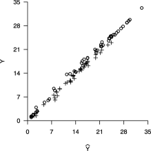(a)	(b)
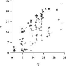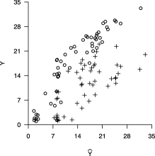(c)	(d)

Figure 8: Plots of the response versus fitted values for the four estimators (a) $\widehat{{\mathbf{R}}}_{\widehat{{\bolds{\Delta}}}}$, (b) $\widehat{{\mathbf{R}}}_{\mathrm{spice}}$, (c) $\widehat{{\mathbf{R}}}_{\mathrm{diag}}$ and (d) $\widehat{{\mathbf{R}}}_{\mathbf{I}}$. Circles represent pork and plus signs represent beef.

Fitting each of the four estimators with $d=1$, we found that $\mathrm{RMS}(1,3,\allowbreak\widehat{{\mathbf{R}}})=41.96$, $41.65$, $0.55$ and $4.66$ for $\widehat{{\mathbf{R}}}=\widehat{{\mathbf{R}}}_{\mathbf{I}}$, $\widehat{{\mathbf{R}}}_{\mathrm{diag}}$, $\widehat{{\mathbf{R}}}_{\widehat{{\bolds{\Delta}}}}$ and $\widehat{{\mathbf{R}}}_{\mathrm{spice}}$. Plots of $Y$ versus $\widehat{Y}$ are shown in Figure 8(a)–(d). The relative signal rates for the four estimators are reflected by the values of $\widehat{\bolds{\Gamma}}{}^{T}\widehat{{\mathbf{W}}}\widehat{\bolds{\Gamma}}=18.4$, $59.2$, $3346.6$ and $69.3$ for $\widehat{{\mathbf{W}}}=(p/\operatorname{tr}(\bolds{\Delta}))\mathbf{I}_{d}$, $\operatorname{diag}^{-1}(\widehat{\bolds{\Delta}})$, $\widehat{\bolds{\Delta}}{}^{-1}$ and $\widehat{\bolds{\Delta}}{}^{-1}_{\widehat{\lambda}}$. The relatively large signal for $\widehat{\bolds{\Delta}}{}^{-1}$ is reflected in the plots of Figure 8.

9 Discussion

The class of estimators that we studied is limited in scope relative to the range of SDR methods presently available for $p=o(n)$ regressions. However, in the broader context of this article, which does not require $p=o(n)$, we introduced the concept of an abundant regression and presented what may be the first $n,p$ asymptotic analysis of a class of SDR methods when the focus is on estimating a reduction ${\mathbf{R}}$ rather than on the underlying central subspace. These ideas can in principle be extended for other SDR methods, and we expect that the same general issues will be encountered. While each of the methods that we studied can perform usefully in the right situation, we judge the SPICE and $\bolds{\Delta}^{-}$ weight matrices to be the best overall, although improvements for nonsparse weight matrices and for regressions with very highly correlated predictors are still needed.

Our simulation results were all based on normal errors to focus the presentation and save space. However, we have also conducted a variety of parallel simulations using Uniform $(0,1)$, $T_{5}$ and $\chi^{2}_{5}$ errors, each centered and appropriately scaled. The results were essentially the same as those with normal errors [Cook, Forzani and Rothman (2012)].

9.1 Penalty functions

Alternative penalty functions may be used for estimating the weight matrix, particularly in scenarios when the inverse error covariance matrix is not sparse. For example, the sparse-seeking penalty function in (5.3), $\lambda\sum_{i\neq j}|\Omega_{ij}|$, could be replaced with the quadratic penalty function,

$$\lambda\Biggl{(}\sum_{i\neq j}\Omega_{ij}^{2}+\alpha\sum_{j=1}^{p}\Omega_{jj}^{2}\Biggr{)},$$ (23)

where $\alpha\in\{0,1\}$ controls whether or not the diagonal of $\bolds{\Omega}$, the inverse error correlation matrix, is penalized. If $\alpha=0$, the general SPICE algorithm developed by Rothman et al. (2008) can efficiently solve (5.3) with the penalty defined in (23). If $\alpha=1$, Witten and Tibshirani (2009) derived an noniterative solution to an equivalent problem to (5.3) with the penalty defined in (23). Recalling that $\varphi_{j}({\mathbf{A}})$ denotes the $j$th eigenvalue of a matrix ${\mathbf{A}}$, let $\eta_{j}=\varphi_{j}(\operatorname{diag}^{-1/2}(\widehat{\bolds{\Delta}})\widehat{\bolds{\Delta}}\operatorname{diag}^{-1/2}(\widehat{\bolds{\Delta}}))$. Witten and Tibshirani showed that the eigenvectors of $\widehat{\bolds{\Omega}}_{\lambda}$ are equivalent to the eigenvectors of $\operatorname{diag}^{-1/2}(\widehat{\bolds{\Delta}})\widehat{\bolds{\Delta}}\operatorname{diag}^{-1/2}(\widehat{\bolds{\Delta}})$ and that $\varphi_{j}(\widehat{\bolds{\Omega}}_{\lambda})=(4\lambda)^{-1}\{(\eta_{j}^{2}+8\lambda)^{1/2}-\eta_{j}\}$.

9.2 Choice of ${\mathbf{f}}$

The general rates given in Proposition 5.1 are not very sensitive to the choice of ${\mathbf{f}}$ since they hold when ${\mathbf{f}}$ satisfies the minimal rank condition (7). Nevertheless, assuming normality and a correct ${\mathbf{f}}$, we obtained the oracle rates of Proposition 6.2, which indicates that there are advantages to pursuing good choices. The methods sketched in Section 3.2 are often useful in practice, but it is also possible to develop semiparametric methods to estimate $\bolds{\xi}$ directly rather than passing through approximations $\bolds{\beta}{\mathbf{f}}$. This might be accomplished iteratively: choose an initial ${\mathbf{f}}$ and construct the corresponding estimates $\bolds{\Gamma}^{1}$, $\bolds{\xi}^{1}=\bolds{\beta}^{1}{\mathbf{f}}$ and ${\mathbf{R}}^{1}_{\widehat{{\mathbf{W}}}}$. A new estimate of $\bolds{\xi}$ can be obtained by smoothing the coordinates of ${\mathbf{R}}^{1}_{\widehat{{\mathbf{W}}}}$ against $Y$, leading to a second reduction estimate ${\mathbf{R}}^{2}_{\widehat{{\mathbf{W}}}}$. The process can now be continued until some convergence criterion is met.

9.3 Variable selection

While we did not incorporate screening or variable selection into our reduction methodology, the potential benefits of those procedures are manifested in our results. Consider, for instance, a regression in which $p^{2/3}$ of the predictors are inactive. Then the oracle rate $\kappa^{-1}=(p/hn)^{-1/2}=n^{1/2}p^{-2/3}$. However, if we remove $p^{1/3}$ of the inactive predictors, the oracle rate is increased to $\kappa^{-1}=n^{1/2}p^{-1/3}$, which should be worthwhile in most applications. Work along these lines is in progress.

References

- Adragni and Cook (2009) {barticle}[mr] \bauthor\bsnmAdragni, \bfnmKofi P.\binitsK. P. and \bauthor\bsnmCook, \bfnmR. Dennis\binitsR. D. (\byear2009). \btitleSufficient dimension reduction and prediction in regression. \bjournalPhilos. Trans. R. Soc. Lond. Ser. A Math. Phys. Eng. Sci. \bvolume367 \bpages4385–4405. \biddoi=10.1098/rsta.2009.0110, issn=1364-503X, mr=2546393 \bptokimsref \endbibitem
- Bai (1999) {barticle}[mr] \bauthor\bsnmBai, \bfnmZ. D.\binitsZ. D. (\byear1999). \btitleMethodologies in spectral analysis of large-dimensional random matrices, a review. \bjournalStatist. Sinica \bvolume9 \bpages611–677. \bptokimsref \endbibitem
- Bickel and Levina (2008a) {barticle}[mr] \bauthor\bsnmBickel, \bfnmPeter J.\binitsP. J. and \bauthor\bsnmLevina, \bfnmElizaveta\binitsE. (\byear2008a). \btitleRegularized estimation of large covariance matrices. \bjournalAnn. Statist. \bvolume36 \bpages199–227. \biddoi=10.1214/009053607000000758, issn=0090-5364, mr=2387969 \bptokimsref \endbibitem
- Bickel and Levina (2008b) {barticle}[mr] \bauthor\bsnmBickel, \bfnmPeter J.\binitsP. J. and \bauthor\bsnmLevina, \bfnmElizaveta\binitsE. (\byear2008b). \btitleCovariance regularization by thresholding. \bjournalAnn. Statist. \bvolume36 \bpages2577–2604. \biddoi=10.1214/08-AOS600, issn=0090-5364, mr=2485008 \bptokimsref \endbibitem
- Bondell and Li (2009) {barticle}[mr] \bauthor\bsnmBondell, \bfnmHoward D.\binitsH. D. and \bauthor\bsnmLi, \bfnmLexin\binitsL. (\byear2009). \btitleShrinkage inverse regression estimation for model-free variable selection. \bjournalJ. R. Stat. Soc. Ser. B Stat. Methodol. \bvolume71 \bpages287–299. \biddoi=10.1111/j.1467-9868.2008.00686.x, issn=1369-7412, mr=2655534 \bptokimsref \endbibitem
- Bura and Cook (2001) {barticle}[mr] \bauthor\bsnmBura, \bfnmEfstathia\binitsE. and \bauthor\bsnmCook, \bfnmR. Dennis\binitsR. D. (\byear2001). \btitleExtending sliced inverse regression: The weighted chi-squared test. \bjournalJ. Amer. Statist. Assoc. \bvolume96 \bpages996–1003. \biddoi=10.1198/016214501753208979, issn=0162-1459, mr=1946367 \bptokimsref \endbibitem
- Chiaromonte and Martinelli (2002) {barticle}[mr] \bauthor\bsnmChiaromonte, \bfnmFrancesca\binitsF. and \bauthor\bsnmMartinelli, \bfnmJessica\binitsJ. (\byear2002). \btitleDimension reduction strategies for analyzing global gene expression data with a response. \bjournalMath. Biosci. \bvolume176 \bpages123–144.\biddoi=10.1016/S0025-5564(01)00106-7, issn=0025-5564, mr=1869195 \bptokimsref \endbibitem
- Chun and Keleş (2010) {barticle}[mr] \bauthor\bsnmChun, \bfnmHyonho\binitsH. and \bauthor\bsnmKeleş, \bfnmSündüz\binitsS. (\byear2010). \btitleSparse partial least squares regression for simultaneous dimension reduction and variable selection. \bjournalJ. R. Stat. Soc. Ser. B Stat. Methodol. \bvolume72 \bpages3–25. \biddoi=10.1111/j.1467-9868.2009.00723.x, issn=1369-7412, mr=2751241 \bptokimsref \endbibitem
- Cook (1994) {bincollection}[auto:STB—2012/02/21—08:54:59] \bauthor\bsnmCook, \bfnmR. D.\binitsR. D. (\byear1994). \btitleUsing dimension-reduction subspaces to identify important inputs in models of physical systems. In \bbooktitleProceedings of the Section on Physical and Engineering Sciences \bpages18–25. \bpublisherAmer. Statist. Assoc., \baddressAlexandria, VA. \bptokimsref \endbibitem
- Cook (1998) {bbook}[mr] \bauthor\bsnmCook, \bfnmR. Dennis\binitsR. D. (\byear1998). \btitleRegression Graphics: Ideas for Studying Regressions Through Graphics. \bpublisherWiley, \baddressNew York. \biddoi=10.1002/9780470316931, mr=1645673 \bptokimsref \endbibitem
- Cook (2004) {barticle}[mr] \bauthor\bsnmCook, \bfnmR. Dennis\binitsR. D. (\byear2004). \btitleTesting predictor contributions in sufficient dimension reduction. \bjournalAnn. Statist. \bvolume32 \bpages1062–1092. \biddoi=10.1214/009053604000000292, issn=0090-5364, mr=2065198 \bptokimsref \endbibitem
- Cook (2007) {barticle}[mr] \bauthor\bsnmCook, \bfnmR. Dennis\binitsR. D. (\byear2007). \btitleFisher lecture: Dimension reduction in regression (with discussion). \bjournalStatist. Sci. \bvolume22 \bpages1–26. \biddoi=10.1214/088342306000000682, issn=0883-4237, mr=2408655 \bptokimsref \endbibitem
- Cook and Forzani (2008) {barticle}[mr] \bauthor\bsnmCook, \bfnmR. Dennis\binitsR. D. and \bauthor\bsnmForzani, \bfnmLiliana\binitsL. (\byear2008). \btitlePrincipal fitted components for dimension reduction in regression. \bjournalStatist. Sci. \bvolume23 \bpages485–501. \biddoi=10.1214/08-STS275, issn=0883-4237, mr=2530547 \bptnotecheck year\bptokimsref \endbibitem
- Cook and Forzani (2009) {barticle}[mr] \bauthor\bsnmCook, \bfnmR. Dennis\binitsR. D. and \bauthor\bsnmForzani, \bfnmLiliana\binitsL. (\byear2009). \btitleLikelihood-based sufficient dimension reduction. \bjournalJ. Amer. Statist. Assoc. \bvolume104 \bpages197–208. \biddoi=10.1198/jasa.2009.0106, issn=0162-1459, mr=2504373 \bptokimsref \endbibitem
- Cook, Forzani and Rothman (2012) {bmisc}[auto:STB—2012/02/21—08:54:59] \bauthor\bsnmCook, \bfnmR. D.\binitsR. D., \bauthor\bsnmForzani, \bfnmL.\binitsL. and \bauthor\bsnmRothman, \bfnmA. J.\binitsA. J. (\byear2012). \bhowpublishedSupplement to “Estimating sufficient reductions of the predictors in abundant high-dimensional regressions.” DOI:\doiurl10.1214/11-AOS962SUPP. \bptokimsref \endbibitem
- Cook, Li and Chiaromonte (2007) {barticle}[mr] \bauthor\bsnmCook, \bfnmR. Dennis\binitsR. D., \bauthor\bsnmLi, \bfnmBing\binitsB. and \bauthor\bsnmChiaromonte, \bfnmFrancesca\binitsF. (\byear2007). \btitleDimension reduction in regression without matrix inversion. \bjournalBiometrika \bvolume94 \bpages569–584. \biddoi=10.1093/biomet/asm038, issn=0006-3444, mr=2410009 \bptokimsref \endbibitem
- Cook and Ni (2005) {barticle}[mr] \bauthor\bsnmCook, \bfnmR. Dennis\binitsR. D. and \bauthor\bsnmNi, \bfnmLiqiang\binitsL. (\byear2005). \btitleSufficient dimension reduction via inverse regression: A minimum discrepancy approach. \bjournalJ. Amer. Statist. Assoc. \bvolume100 \bpages410–428.\biddoi=10.1198/016214504000001501, issn=0162-1459, mr=2160547 \bptokimsref \endbibitem
- Cook and Weisberg (1991) {barticle}[auto:STB—2012/02/21—08:54:59] \bauthor\bsnmCook, \bfnmR. D.\binitsR. D. and \bauthor\bsnmWeisberg, \bfnmS.\binitsS. (\byear1991). \btitleDiscussion of “Sliced inverse regression for dimension reduction” by K.-C. Li. \bjournalJ. Amer. Statist. Assoc. \bvolume86 \bpages382–332. \bptokimsref \endbibitem
- Cook and Yin (2001) {barticle}[mr] \bauthor\bsnmCook, \bfnmR. Dennis\binitsR. D. and \bauthor\bsnmYin, \bfnmXiangrong\binitsX. (\byear2001). \btitleDimension reduction and visualization in discriminant analysis. \bjournalAust. N. Z. J. Stat. \bvolume43 \bpages901–999. \bptokimsref \endbibitem
- d’Aspremont, Banerjee and El Ghaoui (2008) {barticle}[mr] \bauthor\bsnmd’Aspremont, \bfnmAlexandre\binitsA., \bauthor\bsnmBanerjee, \bfnmOnureena\binitsO. and \bauthor\bsnmEl Ghaoui, \bfnmLaurent\binitsL. (\byear2008). \btitleFirst-order methods for sparse covariance selection. \bjournalSIAM J. Matrix Anal. Appl. \bvolume30 \bpages56–66. \biddoi=10.1137/060670985, issn=0895-4798, mr=2399568 \bptokimsref \endbibitem
- Dong and Li (2010) {barticle}[mr] \bauthor\bsnmDong, \bfnmYuexiao\binitsY. and \bauthor\bsnmLi, \bfnmBing\binitsB. (\byear2010). \btitleDimension reduction for non-elliptically distributed predictors: Second-order methods. \bjournalBiometrika \bvolume97 \bpages279–294. \biddoi=10.1093/biomet/asq016, issn=0006-3444, mr=2650738 \bptokimsref \endbibitem
- Friedman, Hastie and Tibshirani (2008) {barticle}[pbm] \bauthor\bsnmFriedman, \bfnmJerome\binitsJ., \bauthor\bsnmHastie, \bfnmTrevor\binitsT. and \bauthor\bsnmTibshirani, \bfnmRobert\binitsR. (\byear2008). \btitleSparse inverse covariance estimation with the graphical lasso. \bjournalBiostatistics \bvolume9 \bpages432–441. \biddoi=10.1093/biostatistics/kxm045, issn=1468-4357, mid=NIHMS248717, pii=kxm045, pmcid=3019769, pmid=18079126 \bptokimsref \endbibitem
- Friedman et al. (2004) {barticle}[auto:STB—2012/02/21—08:54:59] \bauthor\bsnmFriedman, \bfnmJ.\binitsJ., \bauthor\bsnmHastie, \bfnmT.\binitsT., \bauthor\bsnmRosset, \bfnmR.\binitsR., \bauthor\bsnmTibshirani, \bfnmR.\binitsR. and \bauthor\bsnmZhu, \bfnmJ.\binitsJ. (\byear2004). \btitleConsistency in boosting: Discussion. \bjournalAnn. Statist. \bvolume32 \bpages102–107. \bptokimsref \endbibitem
- Fukumizu, Bach and Jordan (2009) {barticle}[mr] \bauthor\bsnmFukumizu, \bfnmKenji\binitsK., \bauthor\bsnmBach, \bfnmFrancis R.\binitsF. R. and \bauthor\bsnmJordan, \bfnmMichael I.\binitsM. I. (\byear2009). \btitleKernel dimension reduction in regression. \bjournalAnn. Statist. \bvolume37 \bpages1871–1905. \biddoi=10.1214/08-AOS637, issn=0090-5364, mr=2533474 \bptokimsref \endbibitem
- Guan and Wang (2010) {barticle}[mr] \bauthor\bsnmGuan, \bfnmYongtao\binitsY. and \bauthor\bsnmWang, \bfnmHansheng\binitsH. (\byear2010). \btitleSufficient dimension reduction for spatial point processes directed by Gaussian random fields. \bjournalJ. R. Stat. Soc. Ser. B Stat. Methodol. \bvolume72 \bpages367–387. \biddoi=10.1111/j.1467-9868.2010.00738.x, issn=1369-7412, mr=2758117 \bptokimsref \endbibitem
- Hall and Li (1993) {barticle}[mr] \bauthor\bsnmHall, \bfnmPeter\binitsP. and \bauthor\bsnmLi, \bfnmKer-Chau\binitsK.-C. (\byear1993). \btitleOn almost linearity of low-dimensional projections from high-dimensional data. \bjournalAnn. Statist. \bvolume21 \bpages867–889. \biddoi=10.1214/aos/1176349155, issn=0090-5364, mr=1232523 \bptokimsref \endbibitem
- Johnstone (2001) {barticle}[mr] \bauthor\bsnmJohnstone, \bfnmIain M.\binitsI. M. (\byear2001). \btitleOn the distribution of the largest eigenvalue in principal components analysis. \bjournalAnn. Statist. \bvolume29 \bpages295–327. \biddoi=10.1214/aos/1009210544, issn=0090-5364, mr=1863961 \bptokimsref \endbibitem
- Johnstone and Lu (2009) {barticle}[mr] \bauthor\bsnmJohnstone, \bfnmIain M.\binitsI. M. and \bauthor\bsnmLu, \bfnmArthur Yu\binitsA. Y. (\byear2009). \btitleOn consistency and sparsity for principal components analysis in high dimensions. \bjournalJ. Amer. Statist. Assoc. \bvolume104 \bpages682–693.\biddoi=10.1198/jasa.2009.0121, issn=0162-1459, mr=2751448 \bptokimsref \endbibitem
- Lam and Fan (2009) {barticle}[mr] \bauthor\bsnmLam, \bfnmClifford\binitsC. and \bauthor\bsnmFan, \bfnmJianqing\binitsJ. (\byear2009). \btitleSparsistency and rates of convergence in large covariance matrix estimation. \bjournalAnn. Statist. \bvolume37 \bpages4254–4278. \biddoi=10.1214/09-AOS720, issn=0090-5364, mr=2572459 \bptokimsref \endbibitem
- Li (1991) {barticle}[mr] \bauthor\bsnmLi, \bfnmKer-Chau\binitsK.-C. (\byear1991). \btitleSliced inverse regression for dimension reduction (with discussion). \bjournalJ. Amer. Statist. Assoc. \bvolume86 \bpages316–342. \bidissn=0162-1459, mr=1137117 \bptokimsref \endbibitem
- Li and Dong (2009) {barticle}[mr] \bauthor\bsnmLi, \bfnmBing\binitsB. and \bauthor\bsnmDong, \bfnmYuexiao\binitsY. (\byear2009). \btitleDimension reduction for nonelliptically distributed predictors. \bjournalAnn. Statist. \bvolume37 \bpages1272–1298. \biddoi=10.1214/08-AOS598, issn=0090-5364, mr=2509074 \bptokimsref \endbibitem
- Li and Li (2004) {barticle}[pbm] \bauthor\bsnmLi, \bfnmLexin\binitsL. and \bauthor\bsnmLi, \bfnmHongzhe\binitsH. (\byear2004). \btitleDimension reduction methods for microarrays with application to censored survival data. \bjournalBioinformatics \bvolume20 \bpages3406–3412. \biddoi=10.1093/bioinformatics/bth415, issn=1367-4803, pii=bth415, pmid=15256406 \bptokimsref \endbibitem
- Li and Yin (2008) {barticle}[mr] \bauthor\bsnmLi, \bfnmLexin\binitsL. and \bauthor\bsnmYin, \bfnmXiangrong\binitsX. (\byear2008). \btitleSliced inverse regression with regularizations. \bjournalBiometrics \bvolume64 \bpages124–131. \biddoi=10.1111/j.1541-0420.2007.00836.x, issn=0006-341X, mr=2422826 \bptokimsref \endbibitem
- Paul (2005) {bmisc}[mr] \bauthor\bsnmPaul, \bfnmDebashis\binitsD. (\byear2005). \btitleNonparametric estimation of principal components. Ph.D. thesis, Dept. Statistics, Stanford Univ. \bidmr=2707156 \bptokimsref \endbibitem
- Ravikumar et al. (2011) {barticle}[mr] \bauthor\bsnmRavikumar, \bfnmPradeep\binitsP., \bauthor\bsnmWainwright, \bfnmMartin J.\binitsM. J., \bauthor\bsnmRaskutti, \bfnmGarvesh\binitsG. and \bauthor\bsnmYu, \bfnmBin\binitsB. (\byear2011). \btitleHigh-dimensional covariance estimation by minimizing -penalized log-determinant divergence. \bjournalElectron. J. Stat. \bvolume5 \bpages935–980. \bptokimsref \endbibitem
- Rothman et al. (2008) {barticle}[mr] \bauthor\bsnmRothman, \bfnmAdam J.\binitsA. J., \bauthor\bsnmBickel, \bfnmPeter J.\binitsP. J., \bauthor\bsnmLevina, \bfnmElizaveta\binitsE. and \bauthor\bsnmZhu, \bfnmJi\binitsJ. (\byear2008). \btitleSparse permutation invariant covariance estimation. \bjournalElectron. J. Stat. \bvolume2 \bpages494–515. \biddoi=10.1214/08-EJS176, issn=1935-7524, mr=2417391 \bptokimsref \endbibitem
- Sæbø et al. (2007) {barticle}[auto:STB—2012/02/21—08:54:59] \bauthor\bsnmSæbø, \bfnmS.\binitsS., \bauthor\bsnmAlmøy, \bfnmT.\binitsT., \bauthor\bsnmAarøe, \bfnmJ.\binitsJ. and \bauthor\bsnmAastveit, \bfnmA. H.\binitsA. H. (\byear2007). \btitleST-PLS: A multi-directional nearest shrunken centroid type classifier via PLS. \bjournalJournal of Chemometrics \bvolume20 \bpages54–62. \bptokimsref \endbibitem
- von Rosen (1988) {barticle}[auto:STB—2012/02/21—08:54:59] \bauthor\bparticlevon \bsnmRosen, \bfnmD.\binitsD. (\byear1988). \btitleThe inverted Wishart distribution. \bjournalScand. J. Stat. \bvolume15 \bpages97–109. \bptokimsref \endbibitem
- Witten and Tibshirani (2009) {barticle}[mr] \bauthor\bsnmWitten, \bfnmDaniela M.\binitsD. M. and \bauthor\bsnmTibshirani, \bfnmRobert\binitsR. (\byear2009). \btitleCovariance-regularized regression and classification for high dimensional problems. \bjournalJ. R. Stat. Soc. Ser. B Stat. Methodol. \bvolume71 \bpages615–636. \biddoi=10.1111/j.1467-9868.2009.00699.x, issn=1369-7412, mr=2749910 \bptokimsref \endbibitem
- Wu and Li (2011) {barticle}[mr] \bauthor\bsnmWu, \bfnmYichao\binitsY. and \bauthor\bsnmLi, \bfnmLexin\binitsL. (\byear2011). \btitleAsymptotic properties of sufficient dimension reduction with a diverging number of predictors. \bjournalStatist. Sinica \bvolume21 \bpages707–730. \biddoi=10.5705/ss.2011.031a, issn=1017-0405, mr=2829852 \bptokimsref \endbibitem
- Xia, Zhang and Xu (2010) {barticle}[mr] \bauthor\bsnmXia, \bfnmYingcun\binitsY., \bauthor\bsnmZhang, \bfnmDixin\binitsD. and \bauthor\bsnmXu, \bfnmJinfeng\binitsJ. (\byear2010). \btitleDimension reduction and semiparametric estimation of survival models. \bjournalJ. Amer. Statist. Assoc. \bvolume105 \bpages278–290. \biddoi=10.1198/jasa.2009.tm09372, issn=0162-1459, mr=2656052 \bptokimsref \endbibitem
- Yuan and Lin (2007) {barticle}[mr] \bauthor\bsnmYuan, \bfnmMing\binitsM. and \bauthor\bsnmLin, \bfnmYi\binitsY. (\byear2007). \btitleModel selection and estimation in the Gaussian graphical model. \bjournalBiometrika \bvolume94 \bpages19–35. \biddoi=10.1093/biomet/asm018, issn=0006-3444, mr=2367824 \bptokimsref \endbibitem
- Zhu, Zhu and Feng (2010) {barticle}[mr] \bauthor\bsnmZhu, \bfnmLi-Ping\binitsL.-P., \bauthor\bsnmZhu, \bfnmLi-Xing\binitsL.-X. and \bauthor\bsnmFeng, \bfnmZheng-Hui\binitsZ.-H. (\byear2010). \btitleDimension reduction in regressions through cumulative slicing estimation. \bjournalJ. Amer. Statist. Assoc. \bvolume105 \bpages1455–1466. \biddoi=10.1198/jasa.2010.tm09666, issn=0162-1459, mr=2796563 \bptokimsref \endbibitem
- Zyskind (1967) {barticle}[mr] \bauthor\bsnmZyskind, \bfnmGeorge\binitsG. (\byear1967). \btitleOn canonical forms, non-negative covariance matrices and best and simple least squares linear estimators in linear models. \bjournalAnn. Math. Statist. \bvolume38 \bpages1092–1109. \bidissn=0003-4851, mr=0214237 \bptokimsref \endbibitem