State transition algorithm

Abstract.

In terms of the concepts of state and state transition, a new heuristic random search algorithm named state transition algorithm is proposed. For continuous function optimization problems, four special transformation operators called rotation, translation, expansion and axesion are designed. Adjusting measures of the transformations are mainly studied to keep the balance of exploration and exploitation. Convergence analysis is also discussed about the algorithm based on random search theory. In the meanwhile, to strengthen the search ability in high dimensional space, communication strategy is introduced into the basic algorithm and intermittent exchange is presented to prevent premature convergence. Finally, experiments are carried out for the algorithms. With 10 common benchmark unconstrained continuous functions used to test the performance, the results show that state transition algorithms are promising algorithms due to their good global search capability and convergence property when compared with some popular algorithms.

Xiaojun Zhou, Chunhua Yang and Weihua Gui

School of Information Science and Engineering

Central South University, Changsha, 410083, China

1. Introduction

The concept of state means to a situation which a material system maintains, and it is characterized by a group of physical qualities. The process of a system turning from a state to another is called state transition, which can be described by a state transition matrix. The idea of state transition was created by a Russian mathematician named Markov when he expected to represent a specific stochastic process (known as Markov process)[22]. Not only in communication theory but also in modern control theory, state transition matrix is of great importance. For instance, in modern control theory, it can determine the stability of a system.
In almost all branches of engineering, including system design, tactical planning, system analysis, process management and control, and model parameter adjustment, optimization techniques have found wide applications[30]. Generally speaking, the methods used for solving such optimization problems can be classified into two categories: deterministic and stochastic, in which, stochastic methods are subdivided into evolutionary algorithms and metaheuristic algorithms. The traditional deterministic algorithms include Hooke-Jeeves pattern search[11] and hill-climbing, evolutionary algorithms contain genetic algorithm (GA)[8, 7], evolutionary programming, evolution strategies, and genetic programming, while metaheuristic algorithms consist of simulated annealing, particle swarm optimization (PSO)[12, 25], differential evolution(DE) algorithm[24], etc. On the other hand, the commonly used numerical algorithms for engineering optimization problems can also be categorized into two classes: direct search methods and gradient-based methods. The direct search methods comprise the simplex search, Powell’s conjugate direction method and random search, while the gradient-based methods include the Newton’s (basic-, modified-, quasi-) and conjugate gradient methods[15]. In the same time, hybrid methods, combining of deterministic and stochastic or direct search and gradient-based, are also proposed to draw on each other’s strengths[2, 29, 16, 32].
According to the No Free Lunch Theorem[28], no search algorithm is better than other algorithms on the space of all possible problems. This paper introduces a new method for optimization of continuous nonlinear functions, which belongs to metaheuristic random search. Because of its foundation on state and state transition, the method is called state transition algorithm (STA)[33, 34]. The algorithm has roots in three main component methodologies. One is the random optimization theory, the others are population-based approach and then space transformation method. In this paper, it focuses on four operators named rotation, translation, expansion and axesion transformation as well as the communication strategy in state transition algorithm. Compared with some state-of-the-art optimization algorithms, RCGA[26], CLPSO[14], and SaDE[20], which are improved versions of GA, PSO and DE, the experimental results show that STAs are comparable and promising algorithms.

2. The basic state transition algorithm

Considering the following unconstrained optimization problem

$$\min_{x\in\Re^{n}}f(x).$$ (1)

In a deterministic view, it usually adopts iterative method to solve the problem

$$x_{k+1}=x_{k}+a_{k}d_{k},$$ (2)

where, $x_{k}$ is the kth iteration point, $a_{k}$ is the kth step size and $d_{k}$ is the kth search direction.
The common selection of a step is by exact line search or inexact line search. While the techniques of search direction include steepest descent method, conjugate gradient methods, Newton’s methods, alternating directions, and conjugate direction methods[31].
In a way, the iterative methods aim to search for a direction and a step in an iteration. Though these methods utilize the gradient information explicitly or implicitly, they have their inherent defects. For one thing, it is computationally difficult. For another, it only indicates the local information. In the view of global optimization, the direction of gradient is just a way standing for direction, and it has no substantial effect on searching for a global optimum. If the iterative method is concerned in a state and state transition way, then an iterative point can be regarded as a state, the process of searching for a direction and a step will equate to a state transition process, and through a state transition, a new state will be created.
In the point of stochastic, it can also understand the evolutionary algorithms and metaheuristic algorithms in a state and state transition way. For example, genetic algorithm, its each individual of a generation can be considered as a state, and the updating process of using genetic operators such as selection, crossover and mutation can equate to state transition processes. In the same way, particle swarm optimization, the flock updating its velocity and position, and differential evolution, adding the difference vector of two randomly chosen vectors to a target vector, can also be regarded as state transition processes.
In terms of the concept of state and state transition, a solution to a specific optimization problem can be described as a state, the operators of optimization algorithms can be considered as state transition, and the process to update current solution will become a state transition process.
Through the above analysis and discussion, it defines the following form of state transition

$$\left\{\begin{array}[]{ll}x_{k+1}=A_{k}x_{k}+B_{k}u_{k}\\ y_{k+1}=f(x_{k+1})\end{array},\right.$$ (3)

where, $x_{k}$ stands for a state, corresponding to a solution to the optimization problem; then, $A_{k}$ and $B_{k}$ are state transition matrixes, which can be regarded as operators of optimization algorithm; $u_{k}$ is the function of state $x_{k}$ and historical states; while $f$ is the cost function or evaluation function.

2.1. State transformation operators

As a matter of fact, operators such as reflection, contraction, expansion and rotation are widely used in simplex optimization method[19, 3, 13], which is especially popular in the fields of chemistry, chemical engineering, and medicine. However, they always fail to lead to continued progress and are not applicable to a wide range of functions.
In the theory of space and transformation, rotation matrices are only defined for two and three dimensional transformation. For example, the two dimensional rotation matrix is $\left[\begin{array}[]{ll}cos\theta&-sin\theta\\ sin\theta&cos\theta\end{array}\right]$.
Using various types of space transformation for reference, in this paper, it defines the following four special state transformation operators to solve continuous function optimization problems.
(1) Rotation transformation

$$x_{k+1}=x_{k}+\alpha\frac{1}{n\|x_{k}\|_{2}}R_{r}x_{k},$$ (4)

where, $x_{k}$ $\in$ $\Re^{n}$, $\alpha$ is a positive constant, called rotation factor; $R_{r}$ $\in$ $\Re^{n\times n}$, is random matrix with its entries obeying the uniform distribution in the range of [-1, 1] and $\|\cdot\|_{2}$ is 2-norm of vector or Euclidean norm. Then, it will prove that the rotation transformation has the function of searching in a hypersphere.

Proof.

$$\begin{split}\|x_{k+1}-x_{k}\|_{2}&=\|\alpha\frac{1}{n\|x_{k}\|_{2}}R_{r}x_{k}\|_{2}\\ &=\frac{\alpha}{n\|x_{k}\|_{2}}\|R_{r}x_{k}\|_{2}\\ &\leq\frac{\alpha}{n\|x_{k}\|_{2}}\|R_{r}\|_{m_{\infty}}\|x_{k}\|_{2}\leq\alpha\end{split}$$ (5)

∎

(2) Translation transformation

$$x_{k+1}=x_{k}+\beta R_{t}\frac{x_{k}-x_{k-1}}{\|x_{k}-x_{k-1}\|_{2}},$$ (6)

where, $\beta$ is a positive constant, called translation factor; $R_{t}$ $\in\Re$ is a random variable with its components obeying the uniform distribution in the range of [0,1]. It is obvious to find the translation transformation has the function of searching along a line from $x_{k-1}$ to $x_{k}$ at the starting point $x_{k}$, with the maximum length of $\beta$.
(3) Expansion transformation

$$x_{k+1}=x_{k}+\gamma R_{e}x_{k},$$ (7)

where, $\gamma$ is a positive constant, called expansion factor; $R_{e}\in\Re^{n\times n}$ is a random diagonal matrix with its elements obeying the Gaussian distribution (in this study, standard normal distribution). It is also obvious to find the expansion transformation has the function of expanding the components in $x_{k}$ to the range of [-$\infty$, +$\infty$], searching in the whole space.
(4) Axesion transformation

$$x_{k+1}=x_{k}+\delta R_{a}x_{k},$$ (8)

where, $\delta$ is a positive constant, called axesion factor; $R_{a}$ $\in\Re^{n\times n}$ is a random diagonal matrix with its entries obeying the Gaussian distribution and only one random position having nonzero value. The axesion transformation aims to search along the axes and strengthens single dimensional search.

2.2. State transformation algorithm

Before the state transition algorithm, it is necessary to introduce the basic random optimization[17, 1, 9, 10]. Considering the above unconstrained optimization problem, the procedure of the basic random optimization can be outlined in the following pseudocode.

1:Initialize feasible solution $x_{0}$, and set $k\leftarrow 0$

2:repeat

3:     $k\leftarrow k+1$

4:     Generate a Gaussian random number vector $r$

5:     $x_{trail}\leftarrow x_{k-1}+r$

6:     if $f(x_{trail})<f(x_{k-1})$ then

7:         $x_{k}\leftarrow x_{trail}$

8:     else

9:         $x_{k}\leftarrow x_{k-1}$

10:     end if

11:until the specified termination criterion is met

For one thing, as a metaheuristic random method, the state transition algorithm is similar to the basic random optimization[17]. The only difference is that a candidate solution set is generated by the four special operators, while a new trail is selected following the same way as that of the basic random optimization, which means that the “greedy criterion” is used in selecting the new state. By the way, a candidate solution set is created by some times of transformation. The times of the transformation or the size of the set is called search enforcement (SE), and the translation operator is only performed when a better new trail is found.
For another, as a stochastic algorithm[5], the dealing with dynamic balance between diversification (exploration of the solution space) and intensification (exploitation of the accumulated knowledge) is also significant in state transition algorithm. Due to their intrinsic properties, the rotation is chosen for exploitation, the expansion is for exploration, the translation is selected as to maintain equilibrium between them, and axesion is proposed to strength the single dimensional search.
The main process of STA is shown in the pseudocode as follows

1:repeat

2:     if $\alpha<\alpha_{\min}$ then

3:         $\alpha\leftarrow\alpha_{\max}$

4:     end if

5:     Best $\leftarrow$ expansion(funfcn,Best,SE,$\beta$,$\gamma$)$\triangleright$ expansion transformation

6:     Best $\leftarrow$ rotation(funfcn,Best,SE,$\alpha$,$\beta$)$\triangleright$ rotation transformation

7:     Best $\leftarrow$ axesion(funfcn,Best,SE,$\beta$,$\delta$)$\triangleright$ axesion transformation

8:     $\alpha\leftarrow\frac{\alpha}{\textit{fc}}$

9:until the specified termination criterion is met

As for detailed explanations, expansion function in above pseudocode is given as follows for example

1:oldBest $\leftarrow$ Best

2:fBest $\leftarrow$ feval(funfcn,oldBest)

3:State $\leftarrow$ op_expand(Best,SE,$\gamma$)

4:[newBest,fGBest] $\leftarrow$ fitness(funfcn,State)

5:if fGBest $<$ fBest then$\triangleright$ greedy criterion

6:     fBest $\leftarrow$ fGBest

7:     Best $\leftarrow$ newBest

8:     State $\leftarrow$ op_translate(oldBest,Best,SE,$\beta$)

9:     [newBest,fGBest] $\leftarrow$ fitness(funfcn,State)

10:     if fGBest $<$ fBest then$\triangleright$ greedy criterion

11:         fBest $\leftarrow$ fGBest

12:         Best $\leftarrow$ newBest

13:     end if

14:end if

2.3. Parameters analysis in STA

In state transition algorithm, there are five important parameters, namely search enforcement(SE), rotation factor $\alpha$, translation factor $\beta$, expansion factor $\gamma$ and axesion factor $\delta$. It is easy to understand that the larger the search enforcement, the higher the intensity of search, and vise versa. However, the larger search enforcement will cause larger computational complexity. In this paper, the search enforcement is recommended to use the same size as the dimension of the optimization problem.
When SE is constant, taking the exploration and exploitation into consideration, the strategy of adjusting parameters of the four operators is significant. To make the deeper exploitation, the smaller rotation factor is needed. Especially, the rotation factor will vary in a declining way from a positive constant till zero to gain a high precision solution. In the meanwhile, there are two schemes to regulate the $\alpha$. One is to adjust the parameter in an inner loop, namely, decreasing the rotation factor from a start constant to the end in the operation of rotation transformation[33]. The other is to adjust the parameters in an outside loop, that is to say, decreasing the rotation factor according to the iterations. To balance the global search and local search timely, the latter scheme is adopted in the paper; however, the rotation factor is decreasing itself from a maximum value to a minimum value in an exponential way with base fc, which is called lessening coefficient[34], as described in the pseudocode of STA. By the way, extra tests have testified the effectiveness of the scheme.
As for the remained control parameters, for example, the larger the translation factor, the longer STA searches along a straight line. However, the magnitude of translation factor has great influence on exploitation and exploration. The large translation factor will facilitate the exploration, while the small translation factor benefits the exploitation. Similarly, the same phenomenon exists in the selection of expansion and axesion factors. Taking the complexity of adjusting strategies for these control parameters into consideration, we keep them fixed in current version of STA for simplicity.

2.4. The convergence analysis of STA

The convergence of stochastic optimization algorithms has been heatedly discussed. For instance, genetic algorithm was analyzed by means of homogeneous finite Markov chain[21], particle swarm optimization was studied to investigate particle trajectories in a discrete system view[4], and convergence property of differential evolution was also discussed in[24].
As a metaheuristic random optimization algorithm, the convergence analysis of STA will follow the same way as random search methods. In fact, the probability of random search algorithm for finding global minimum being equal to 1 was stated by Solis and Wets[23]. That is to say, the STA will satisfy the similar convergence performance of random optimization algorithm, and readers who are interested in convergence analysis are referred to their work for details.

3. Communication strategy into state transition algorithm

In a way, the basic state transition algorithm is individual-based, and an individual searches in its neighborhood. The difference between the basic state transition algorithm and other random optimizations is that the search space is normalized or specialized.
The population-based approach is prevalent in metaheuristic algorithms, such as genetic algorithm, particle swarm optimization and differential evolution. Let’s name the basic state transition algorithm STAI, the improved state transition algorithm based on population is called STAII with the number of states denoted as SN. In the meanwhile, some communication strategies are necessary to manage the individuals for sharing information, which is important in population-based methods.

3.1. Crossover operator

Individual communication can be implemented in various ways, of which crossover operation is quite common, especially in genetic algorithms.
Let $X_{1}$ and $X_{2}$ be individual components of current generation, $Y_{1}$ and $Y_{2}$ are the offspring components, some canonical crossover operators are displayed in the following.
(1) Michalewicz’s arithmetical crossover[18]

$$\left\{\begin{array}[]{ll}Y_{1}=\alpha X_{1}+(1-\alpha)X_{2}\\ Y_{2}=\alpha X_{2}+(1-\alpha)X_{1}\end{array},\right.$$ (9)

where, $\alpha$ is either a constant or a variable whose value depends on the age of population.
(2) Wright’s linear crossover[27]

$$Y_{1}=1.5X_{1}-0.5X_{2},Y_{2}=-0.5X_{1}+1.5X_{2},Y_{3}=(X_{1}+X_{2})/2$$ (10)

(3) Kalyanmoy Deb’s simulated binary crossover[6]

$$\left\{\begin{array}[]{ll}Y_{1}=0.5[(1-\beta)X_{1}+(1+\beta)X_{2}]\\ Y_{2}=0.5[(1+\beta)X_{1}+(1-\beta)X_{2}]\end{array},\right.$$ (11)

where, $\beta$ is a random variable, obeying the following probability distribution

$$\begin{cases}p(\beta)=0.5(\eta_{c}+1)\beta^{\eta_{c}}&0\leq\beta\leq 1,\\ p(\beta)=0.5(\eta_{c}+1)\frac{1}{\beta^{\eta_{c}+2}}&\beta>1,\end{cases}$$ (12)

here, $p(\cdot)$ is the probability density function, $\eta_{c}$ is the distribution index, which determine how well spread the children will be inherited from their parents.
(4) The proposed crossover

$$\left\{\begin{array}[]{ll}Y_{1}=\delta X_{1}+(1-\delta)X_{2},\\ Y_{2}=\eta X_{1}+(1-\eta)X_{2},\end{array}\right.$$ (13)

where, $\delta$ and $\eta$ are independent variables, which obey the 0-1 distribution.
In this proposed crossover, crossover operation means for each component of a pair of individuals, components exchange or maintain their information completely.

3.2. Intermittent exchange

Different from other population based algorithms, all of the individuals in STAII are elites, and they develop themselves trough state transformation, which is referred as self learning. When the communication strategy is introduced, the individual can contact with each other to better develop themselves. However, it may bring about some disadvantageous effects. If the frequency of individual communication is too high, individuals are apt to imitate each other utterly, which will cause premature convergence. In this paper, intermittent exchange is proposed to solve the issue, that is to say, individual communication occurs at a certain frequency, where the frequency is named communication frequency (CF).
The communication strategy is adopted to share information among individuals, and it is regulated by communication frequency. If CF is small enough, it will equate the situation without the communication strategy. When CF is too large, individuals are easily trapped into imitating each other, causing the premature convergence, that is to say, a moderate CF is appropriate. In this paper, we recommend to use the same magnitude as square root of the maximum iterations.
When the exchange condition is satisfied, the proposed crossover operator will be performed. Each state will communicate with all of the other states, to make sure that useful information is completely shared.

3.3. The framework of STA with communication strategy

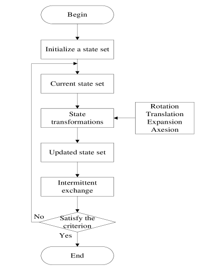
Through the above discussion and analysis, by introducing in communication strategy, the pseudocode of the kernel of state transition algorithm can be described as shown in the following

1:repeat

2:     if $\alpha<\alpha_{\min}$ then

3:         $\alpha\leftarrow\alpha_{\max}$

4:     end if

5:     State $\leftarrow$ self_learning(funfcn,State,SE,$\alpha$,$\beta$,$\gamma$,$\delta$)$\triangleright$ self learning

6:     $\alpha\leftarrow\frac{\alpha}{\textit{fc}}$

7:     if mod(iter,CF)==0 then$\triangleright$ intermittent exchange

8:         State $\leftarrow$ communication(funfcn,State)

9:     end if

10:     [Best,fBest] $\leftarrow$ fitness(funfcn,State)

11:until the specified termination criterion is met

In the process of the algorithm, the $self\_learning$ means each state in the state set will be performed on four state transformation operators, while in $communication$ function, the intermittent exchange is adopted at intervals. The flowchart of the algorithm is outlined in Figure 1.

Figure 1. the flowchart of STAII

4. Experiments and results

To compare the proposed state transition algorithm with previously mentioned RCGA, CLPSO and SaDE, two experiments are arranged. The first experiment is mainly for two dimensional functions, and the other focuses on ten dimensional functions test. In the same time, both STAI and STAII are carried out, for comparison with other algorithms as well as themselves.

4.1. Test functions

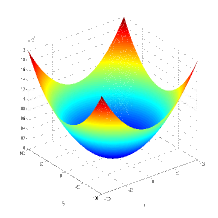
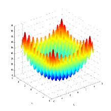
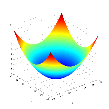
In order to test the performance of STA, ten common benchmark functions are selected for the experiment. Seven functions are multidimensional functions of various modals and the other three are two dimensional functions, which are listed in Table 1, while the landscapes of two dimensional functions are plotted in Figure 2.

Table 1. Benchmark functions for test in this paper

Name of function	Function definition	Range	$f_{min}$
Spherical	$~{}f_{1}=\sum_{i=1}^{n}x_{i}^{2}$	[-100,100]	0
Rastrigin	$~{}f_{2}=\sum_{i=1}^{n}(x_{i}^{2}-10cos(2\pi x_{i})+10)$	[-5.12,5.12]	0
Griewank	$~{}f_{3}=\frac{1}{4000}\sum_{i=1}^{n}x_{i}^{2}-\prod_{i}^{n}cos|\frac{x_{i}}{\sqrt{i}}|+1$	[-600,600]	0
Rosenbrock	$~{}f_{4}=\sum_{i=1}^{n}(100(x_{i+1}-x_{i}^{2})^{2}+(x_{i}-1)^{2})$	[-30,30]	0
Schewefel	$~{}f_{5}=\sum_{i=1}^{n}[-x_{i}sin(\sqrt{|x_{i}|})]$	[-500,500]	-418.9829n
Ackley	$\begin{array}[]{l}f_{6}=20+e-20exp(-0.2\sqrt{\frac{1}{n}\sum_{i=1}^{n}x_{i}^{2}})\\ -exp(\frac{1}{n}\sum_{i=1}^{n}cos(2\pi x_{i}))\end{array}$	[-32,32]	0
Michalewicz	$~{}f_{7}=\sum_{i=1}^{n}sin(x_{i})sin(\frac{ix_{i}^{2}}{\pi})^{20}$	$[0,\pi]$	-
Schaffer	$~{}f_{8}=0.5+\frac{sin(\sqrt{x_{1}^{2}+x_{2}^{2}})^{2}-0.5}{(1+0.001(x_{1}^{2}+x_{2}^{2}))^{2}}$	[-100,100]	0
Easom	$\begin{array}[]{l}f_{9}=-cos(x_{1})cos(x_{2})\times\\ exp(-(x_{1}-\pi)-(x_{2}-\pi))\end{array}$	[-100,100]	-1
Goldstein-Price	$\begin{array}[]{l}f_{10}=[1+(x_{1}+x_{2}+1)^{2}(19-14x_{1}+3x_{1}^{2}\\ -14x_{2}+6x_{1}x_{2}+3x_{2}^{2})]\times[30+(2x_{1}-3x_{2})^{2}\\ (18-32x_{1}+12x_{1}^{2}+48x_{2}-36x_{1}x_{2}+27x_{2}^{2})]\end{array}$	[-2,2]	3

(a) $f_{1}$

(b) $f_{2}$

(c) $f_{3}$

(d) $f_{4}$

(e) $f_{5}$

(f) $f_{6}$

(g) $f_{7}$

(h) $f_{8}$

(i) $f_{9}$

(j) $f_{10}$

Figure 2. Plots of the two dimensional functions from $f_{1}$ to $f_{10}$

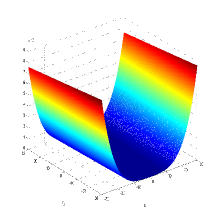
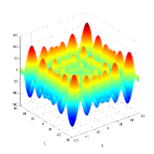
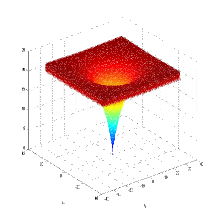
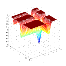
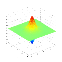
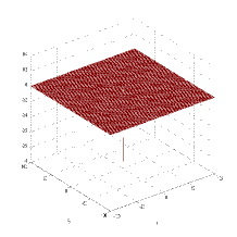
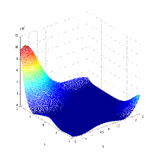
4.2. Parameters setting

All of the algorithms were run on MATLAB (Version R2010b) software platform. For simplicity and normalization, the experiment specifies all the control parameters of transformation operators in STAI and STAII starting at 1. Commonly, the variation of a parameter follows a linear, exponential or a logistic way. In this paper, the exponential way is accepted for its rapidity, of which the base is 2 in the experiment. In view of the operational precision of MATLAB in short format, the minimum $\alpha$ factor fixed at 1e-4 is enough for the situation.
As for RCGA, we use the same parameter settings as in[26]. Then, for CLPSO and SaDE, we use the MATLAB codes provided by the author in[14, 20] with minor revisions for this experiment.
Programs were run independently for 30 trails, and for each trail, the population scale is 30, and the maximum iteration is 1000. The detailed parameters of STAI and STAII are shown in Table 2 and Table 3, respectively.

Table 2. Parameters setting of STAI

Parameter	Value
SE	30
$\alpha$	1 $\rightarrow$ 1e-4
$\beta$	1
$\gamma$	1
$\delta$	1
fc	2

Table 3. Parameters setting of STAII

Parameter	Value
SN	30
SE	10
CF	50
$\alpha$	1 $\rightarrow$ 1e-4
$\beta$	1
$\gamma$	1
$\delta$	1
fc	2

4.3. Results and discussion

For comparison, some common statistics are introduced. The best means the minimum of the results, the worst indicates the maximum of the results, and then it follows the mean, median and st.dev.(standard deviation). In some way, these statistics are able to evaluate the search ability and solution accuracy, reliability and convergence as well as stability. To be more specific, the best indicates the global search ability and solution accuracy, the worst and the mean signify the reliability and convergence, while the median and st.dev. correspond to the stability.
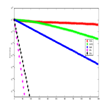
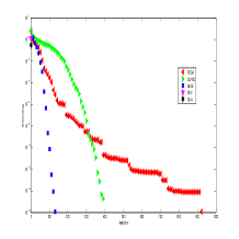
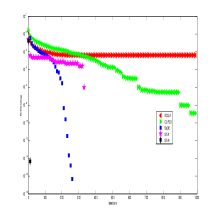
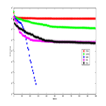
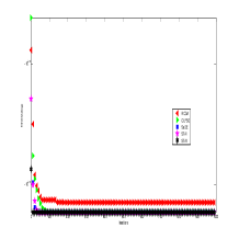
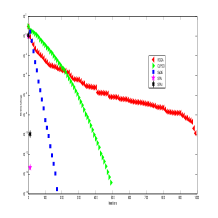
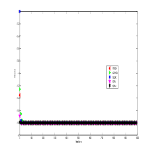
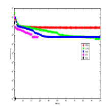
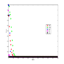
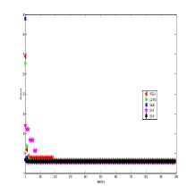
Results for two dimensional functions optimization are listed in Table 4, while results for ten dimensional functions optimization can be found in Table 5. On the other hand, illustrations of the average fitness in 30 simulations are given in Figure 3 and Figure 4 for two dimensional and ten dimensional functions, respectively. The average fitness curve can visually depict the search ability and convergence performance. In the following paragraphs the analysis of the results for each functions will be discussed separately.

Table 4. Comparisons among various algorithms on test functions(2D)

Fcn	Statistic	RCGA	CLPSO	SaDE	STAI	STAII
	best	1.5795e-028	2.7344e-091	2.9229e-196	0	0
	median	4.9090e-024	2.6808e-087	4.2548e-189	0	0
$f_{1}$	mean	1.5458e-022	5.9580e-082	6.6729e-188	0	0
	worst	2.5849e-021	1.7771e-080	9.6210e-187	0	0
	st.dev.	4.7939e-022	3.2440e-081	0	0	0
	best	0	0	0	0	0
	median	0	0	0	0	0
$f_{2}$	mean	0	0	0	0	0
	worst	0	0	0	0	0
	st.dev.	0	0	0	0	0
	best	0	0	0	0	0
	median	0.0074	0	0	0	0
$f_{3}$	mean	0.0042	1.2460e-009	0	0	0
	worst	0.0074	3.7377e-008	0	0	0
	st.dev.	0.0037	6.8241e-009	0	0	0
	best	7.0832e-008	9.2890e-010	0	1.0092e-012	4.2592e-014
	median	0.0085	3.9984e-007	0	1.0900e-011	3.9400e-012
$f_{4}$	mean	1.0364	3.9260e-005	0	1.2571e-011	4.4217e-012
	worst	26.2801	6.3652e-004	0	4.7764e-011	1.4588e-011
	st.dev.	4.7802	1.4088e-004	0	1.0692e-011	3.9023e-012
	best	-837.9658	-837.9658	-837.9658	-837.9658	-837.9658
	median	-837.9658	-837.9658	-837.9658	-837.9658	-837.9658
$f_{5}$	mean	-822.1740	-837.9658	-837.9658	-837.9658	-837.9658
	worst	-719.5274	-837.9658	-837.9658	-837.9658	-837.9658
	st.dev.	40.9496	0	0	1.5939e-013	1.0970e-013
	best	2.0428e-014	-8.8818e-016	-8.8818e-016	-8.8818e-016	-8.8818e-016
	median	3.1681e-012	-8.8818e-016	-8.8818e-016	-8.8818e-016	-8.8818e-016
$f_{6}$	mean	4.7516e-011	-8.8818e-016	-8.8818e-016	-8.8818e-016	-8.8818e-016
	worst	9.6937e-010	-8.8818e-016	-8.8818e-016	-8.8818e-016	-8.8818e-016
	st.dev.	1.8319e-010	0	0	0	0
	best	-1.8013	-1.8013	-1.8013	-1.8013	-1.8013
	median	-1.8013	-1.8013	-1.8013	-1.8013	-1.8013
$f_{7}$	mean	-1.8013	-1.8013	-1.8013	-1.8013	-1.8013
	worst	-1.8013	-1.8013	-1.8013	-1.8013	-1.8013
	st.dev.	9.0336e-016	9.0336e-016	9.0336e-016	2.2063e-011	7.6618e-012
	best	0	0	0	0	0
	median	0.0097	9.3299e-012	0	0	0
$f_{8}$	mean	0.0071	4.1836e-004	6.4773e-004	0	0
	worst	0.0097	0.0097	0.0097	0	0
	st.dev.	0.0044	0.0018	0.0025	0	0
	best	-1.0000	-1.0000	-1.0000	-1.0000	-1.0000
	median	-1.0000	-1.0000	-1.0000	-1.0000	-1.0000
$f_{9}$	mean	-1.0000	-1.0000	-1.0000	-1.0000	-1.0000
	worst	-1.0000	-1.0000	-1.0000	-1.0000	-1.0000
	st.dev.	0	0	0	1.0124e-012	2.6511e-013
	best	3.0000	3.0000	3.0000	3.0000	3.0000
	median	3.0000	3.0000	3.0000	3.0000	3.0000
$f_{10}$	mean	3.0000	3.0000	3.0000	3.0000	3.0000
	worst	3.0000	3.0000	3.0000	3.0000	3.0000
	st.dev.	2.5135e-015	1.5317e-015	1.2669e-015	2.5697e-010	1.2191e-010

(a) $f_{1}$

(b) $f_{2}$

(c) $f_{3}$

(d) $f_{4}$

(e) $f_{5}$

(f) $f_{6}$

(g) $f_{7}$

(h) $f_{8}$

(i) $f_{9}$

(j) $f_{10}$

Figure 3. Average fitness of the two-dimensional functions from $f_{1}$ to $f_{10}$

Table 5. Comparisons among various algorithms on test functions(10D)

Fcn	Statistic	RCGA	CLPSO	SaDE	STAI	STAII
	best	4.0118e-012	1.5229e-012	1.0686e-053	0	0
	median	4.1019e-011	5.3464e-011	1.6873e-051	0	0
$f_{1}$	mean	8.4302e-011	6.0282e-011	3.5549e-051	0	0
	worst	5.6332e-010	1.6279e-010	2.7214e-050	0	0
	st.dev.	1.1766e-010	4.9198e-011	6.1159e-051	0	0
	best	1.0814e-011	1.9806e-006	0	0	0
	median	2.9849	1.0401e-005	0	0	0
$f_{2}$	mean	2.6864	2.7769e-005	0.0332	0	0
	worst	5.9697	2.5009e-004	0.9950	0	0
	st.dev.	1.5491	4.7363e-005	0.1817	0	0
	best	3.2914e-010	2.6061e-005	0	0	0
	median	0.0492	0.0019	0	0	0
$f_{3}$	mean	0.0582	0.0038	5.7529e-004	0.0166	0
	worst	0.1699	0.0166	0.0099	0.0738	0
	st.dev.	0.0439	0.0045	0.0022	0.0260	0
	best	0.0662	0.6841	8.3515e-012	2.6607e-005	7.3949e-005
	median	7.2483	4.0404	3.4637e-004	1.7823	0.2809
$f_{4}$	mean	7.0110	4.3775	0.3415	2.3266	0.4095
	worst	9.2754	12.3253	3.9866	21.8603	1.5228
	st.dev.	1.4466	2.8042	1.0098	3.7249	0.4124
	best	-3.9530e+003	-4.1898e+003	-4.1898e+003	-4.1898e+003	-4.1898e+003
	median	-3.8345e+003	-4.1898e+003	-4.1898e+003	-4.1898e+003	-4.1898e+003
$f_{5}$	mean	-3.7832e+003	-4.1898e+003	-4.1898e+003	-4.1898e+003	-4.1898e+003
	worst	-3.3608e+003	-4.1898e+003	-4.1898e+003	-4.1898e+003	-4.1898e+003
	st.dev.	151.3665	5.5006e-008	2.7751e-012	1.1734e-011	1.9256e-012
	best	6.6339e-007	1.5533e-006	-8.8818e-016	-8.8818e-016	-8.8818e-016
	median	2.8352e-006	4.0369e-006	2.6645e-015	-8.8818e-016	-8.8818e-016
$f_{6}$	mean	3.1524e-006	4.8197e-006	2.3093e-015	2.9606e-016	-8.8818e-016
	worst	9.6980e-006	1.3052e-005	2.6645e-015	2.6645e-015	-8.8818e-016
	st.dev.	2.1010e-006	3.2984e-006	1.0840e-015	1.7034e-015	0
	best	-9.6154	-9.6601	-9.6602	-9.6602	-9.6602
	median	-9.2604	-9.6598	-9.6602	-9.6602	-9.6602
$f_{7}$	mean	-9.2425	-9.6588	-9.6513	-9.1797	-9.6602
	worst	-8.7143	-9.6549	-9.6135	-7.6602	-9.6602
	st.dev.	0.2265	0.0018	0.0173	0.6044	1.9138e-009

(a) $f_{1}$

(b) $f_{2}$

(c) $f_{3}$

(d) $f_{4}$

(e) $f_{5}$

(f) $f_{6}$

(g) $f_{7}$

Figure 4. Average fitness of the ten-dimensional functions from $f_{1}$ to $f_{7}$

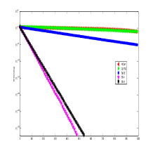
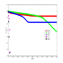
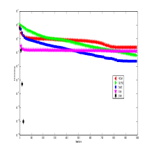
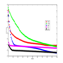
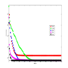
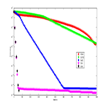
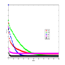
Spherical Function: as can be seen from the results, all of the algorithms can find the global optimum with high solution precision and have good reliability as well as stability for this function in terms of two and ten dimensions. But the STAI and STAII are able to search much deeper than other three algorithms, which can also be observed in subfigure (A) of Figure 3 and Figure 4. In the subfigure (A), we can see that STAs can converge much faster than the remained methods. While for STAI and STAII, it is found that STAI has a little faster convergence performance than that of STAII.
Rastrigin Function: we can see from the results that all of the algorithms can find the global optimum and have good reliability as well as stability in two dimension. For the ten dimensional problem, the global optimum can also be found by all algorithms; however, STAI and STAII have better statistical performances than other three algorithms especially described by the worst. RCGA and SaDE can not achieve the best occasionally, and the mean of RCGA is not satisfactory. From subfigure (B) of Figure 3 and Figure 4, we can also find that STAs converge much faster than other algorithms, and higher solution precision can be obtained. In this time, the process of STAII is slightly faster than that of STAI.
Griewank Function: from the results, we can find that most algorithms have the ability to achieve the best and have both reliability and stability in the two dimensional function except the RCGA. While for the ten-dimension function, these methods are able to find the global optimum but the statistical performances are not satisfactory except STAII, the results of which are excellent. In subfigure (C) of Figure 3 and Figure 4, it can be found that STAII converge fastest and have highest solution precision of all.
Rosenbrock Function: all of the algorithms have no problem to find the global optimum for this function in two-dimensional space, but the worst of RCGA indicate that it is not reliable and a bit deficient for the function. Regarding corresponding ten dimensional problem, only SaDE and STAs can find the best with a low probability. In this case, SaDE achieves best results, followed by STAII. From subfigure (D) of Figure 3 and Figure 4, we can find that STAs still converge faster than other algorithm but with not higher solution precision than SaDE. Compared with STAI, STAII have much better statistical performances, which are indicated by the worst and the mean.
Schewefel Function: as for the function, only RCGA can not find the global optimum for both two and ten dimensions; furthermore, the median and st.dev. also show that the RCGA is not stable and reliable for this function. Other algorithms achieve the best as well as good reliability and stability because the st.dev approaches zero for these methods. From subfigure (E) of Figure 3 and Figure 4, the faster convergence speed belongs to the STAs as well. While for STAs, it shows that STAII converge faster than STAI for the function.
Ackley Function: it seems that all of the algorithms have no problem in finding the global optimum for the function in terms of two and ten dimensions. The statistical performances of results are satisfactory for all methods because the st.dev. approaches zero. In subfigure (F) of Figure 3 and Figure 4, we can find that STAs also have faster convergence speed than other algorithms and the solution precision is also higher for STAs when compared with others.
Michalewicz Function: all of the algorithms can achieve the global optimum for this function in two dimension, and the statistical performances is satisfactory in this case. While for the function with ten dimension, only STAII are able to achieve the same statistics as the results in two dimensional function. More specifically, RCGA and CLPSO are not able to find the best. The worst of STAI show that it is not reliable sometimes.
Schaffer Function: the global optimum can be found by all the algorithms; however, only STAs can achieve reliable and stable performance for this function, as indicated by the mean and the st.dev.. Other methods fail to find the best occasionally, which is described by the worst, that is to say, other algorithm are not reliable for the function. In the case, STAII converge much faster than STAI, as illustrated by subfigure (H).
Easom Function: all of the algorithms are able to find the global optimum with a high probability. The st.dev. indicates that the statistical performance are also fine for all methods. The subfigure (I) of Figure 3 shows that STAs have better convergence performance again.
Goldstein-Price Function: as described in Table 4, global optimum can be found by all algorithms, the results of which are satisfactory because the st.dev. approaches zero. The subfigure (J) of Figure 3 shows that the convergence speed is fine for all methods but the STAs are much better to some extent.
Over all, some explanations can be given on the behavior of average fitness curves. As shown in Figure 3 and Figure 4, the curves of STAs change steadily during the iteration process in most cases, There are two reasons that account for the phenomenon. Firstly, the rotation guarantees the steady decrease of the curves because the rotation factor changes from a maximum value to a minimum value in a periodical way, which prevents current best state from changing sharply. If other transformations do not work, then rotation will help searching in depth with a high precision. Secondly, expansion and translation are beneficial for searching in a new area, while the axesion is proposed to strength the single dimensional search, which are all advantageous for the decrease of the curves.
But every once in a while, especially described by the average fitness of $f_{4}$ and $f_{7}$ in ten dimension, STAs fail to find the global optimum. As declared in Part 2.2, rotation transformation is used for local search, expansion, translation, and axesion are helpful for global search. In current STAs, their control parameters(transformation factors) are determined by experimental experience for simplicity. The failure of STAs for $f_{4}$ and $f_{7}$ occasionally indicate that the global search transformations need to be deeply studied. Anyway, the smaller rotation factor will facilitate the exploitation and the bigger expansion, translation and axesion factors will benefit the exploration, though how to balance them are still pending. Regarding the influence of the CF, we can find that STAII has stronger search ability than STAI as the introducing of intermittent exchange. As illustrated by the average fitness curves, the fitness by STAII can still decrease even if that of STAI is already steady, that is to say, the communication strategy can help share information and prevent premature convergence. If the CF is larger, more information will be shared, and if the CF is small, self development will be enhanced.
By the way, the searching time required for STAs is infinity in theory, which is the consequence of random search methodology. However, in practice, we can stop the iteration process by presetting some criteria, for example, the prescribed maximum iterations, or when the fitness is unchanged for a number of times. In this paper, the maximum iterations is used.

5. Conclusion

Based on state and state transition, the STA, not only has a simple form but also possess clear geometric significance, which is easy for understanding. Concerning the continuous function optimization problems, it presents the state transformations including rotation transformation, translation transformation and expansion transformation as well as axesion transformation. The paper focuses on the unconstrained optimization problems, and it studies mainly on the approaches of transformations. Furthermore, to enhance its performance in high dimensional functions optimization, communication strategy has been introduced, and the intermittent exchange is proposed to strength the search ability as well as prevent premature convergence. Using 10 benchmark functions for testing, compared with some distinguished optimization algorithms, it shows that STAs have fine performance in terms of global search ability and convergence accuracy, which confirms the effectiveness of the proposed algorithms.
On the other hand, distinguished from other population-based algorithms, STA is not originated from simulating natural intelligence, but it takes advantages of the space structure of a function, which opens a new window for optimization. In the paper, control parameters of STAs are not studied deeply, and they are only determined by the experimental experience or for simplicity. In our future work, these problems will be focused on to better develop the state transition algorithms.

References

- [1] (MR1441281) [10.1016/S0378-4754(96)00069-9] G. Albeanu, A monte carlo approach for control search, Mathematics and Computers in Simulation, 43 (1997), 223–228.
- [2] H. A. Abbass, A. M. Bagirov and J. Zhang, The discrete gradient evolutionary strategy method for global optimization, in “Proceedings of IEEE Congress on Evolutionary Computation”, 1 (2003), 435–442.
- [3] [10.1016/S0003-2670(00)85224-1] D. D. Burgess, Rotation in simplex optimization, Analytica Chimica Acta, 181 (1986), 97–106.
- [4] (MR2212427) [10.1016/j.ins.2005.02.003] F. V. Berth and A. P. Engelbrecht, A study of particle swarm optimization particle trajectories, Information Sciences, 176 (2006), 937–971.
- [5] P. Collet and J. P. Rennard, “Stochastic Optimization Algorithms,” Handbook of Research on Nature Inspired Computing for Economics and Management, 2006.
- [6] (MR1381067) K. Deb and R. B. Agrawal, Simulated binary crossover for continuous search space, Complex systems, 9 (1995), 115–148.
- [7] R. C. Eberhart and Y. H. Shi, Comparison between genetic algorithms and particle swarm optimization, in “Annual Conference on Evolutionary programming”, San Diego, (1998), 611–616.
- [8] D. E. Goldberg, “Genetic Algorithms in Search, Optimization, and Machine Learning,” Reading: Addison-Wesley, 1989.
- [9] (MR2208016) [10.1016/j.amc.2005.05.002] C. Hamzacebi and F. Kutay, A heuristic approach for finding the global minimum: Adaptive random search technique, Applied Mathematics and Computation, 173 (2006), 1323–1333.
- [10] [10.1016/j.apm.2006.08.015] C. Hamzacebi and F. Kutay, Continous functions minimization by dynamic random search technique, Applied Mathematical Modeling, 31 (2007), 2189–2198.
- [11] R. Hooke and T. A. Jeeves, Direct search solution of numerical and statistical problems, Journal of the Association for Computing Machinery(ACM), 8 (1961), 212–229.
- [12] J. Kennedy and R. C. Eberhart, Particle swarm optimization, in “Proceedings of IEEE International Conference on Neural Networks”, IEEE Service Center, Piscataway, NJ, (1995), 1942–1948.
- [13] (MR1662563) J. C. Lagarias, J. A. Reeds, M. H. Wright and P. E. Wright, Convergence properties of the Nelder-Mead simplex method in low dimensions, SIAM J. OPTIM., 9 (1998), 112–147.
- [14] J. J. Liang, A. K. Qin, P. N. Suganthan and S. Baskar, Comprehensive learning particle swarm optimizer for global optimization of multimodal functions, IEEE Transaction on Evolutionary Computation, 10 (2006), 281–295.
- [15] J. Y. Li and R. R. Rhinehart, Heuristic random optimization, Computers and Chemical Engineering, 22 (1998), 427–444.
- [16] (MR2379918) T. W. Leung, C. K. Chan and M. D. Troutt, A mixed simulated annealing-genetic algorithm approach to the multi-buyer multi-item joint replenishment problem: advantages of meta-heuristics, Journal of Industrial and Management Optimization, 4 (2008), 53–66.
- [17] (MR0178974) J. Matyas, Random optimization, Automation and Remote Control, 26 (1965), 246–253.
- [18] [10.1016/0898-1221(92)90094-X] Z. Michalewicz, A modified genetic algorithm for optimal control problems, Computers Math. Applic, 23 (1992), 83–94.
- [19] J. A. Nelder and R. Mead, A simplex method for function minimization, Computer Journal, 7 (1965), 308–313.
- [20] A. K. Qin, V. L. Huang, and P. N. Suganthan, Differential evolution algorithm with strategy adaptation for global numerical optimization, IEEE Transactions on Evolutionary Computation, 13 (2009), 398–417.
- [21] G. Rudolph, Convergence analysis of canonical genetic algorithms, IEEE Transactions on Neural Networks, 5 (1994), 96–101.
- [22] D. W. Stroock, “An Introduction to Markov Processes,” Beijing: World Publishing Corporation, 2009.
- [23] (MR0618961) F. J. Solis and R. J. B. Wets, Minimization by random search techniques, Mathematics of Operations Research, 6 (1981), 19–30.
- [24] (MR1479553) [10.1023/A:1008202821328] R. Storn and K. V. Price, Differential evolutionary-A simple and efficient heuristic for global optimization over continous spaces, Journal of global optimization, 11 (1997), 341–359.
- [25] Y. H. Shi and R. C. Eberhart, Empirical study of particle swarm optimization, in “Proceedings of the IEEE Congress on Evolutionary Computation”, IEEE Press, Seoul, Korea, (2001), 1945–1950.
- [26] T. D. Tran and G. G. Jin, Real-coded genetic algorithm benchmarked on noiseless black-box optimization testbed, in “Workshop Proceedings of the Genetic and Evolutionary Computation Conference”, (2010), 1731–1738.
- [27] (MR1147427) A. H. Wright, Genetic algorithms for real parameter optimization, in “Foundations of Genetic Algorithms” (Ed. G. J. E. Rawlins), (1991), 205–220.
- [28] D. H. Wolpert and W. G. Macready, No free lunch theorems for optimization, IEEE Transactions on Evolutionary Computation, 1 (1997), 67–82.
- [29] (MR2059088) [10.1023/B:JOGO.0000015313.93974.b0] K. F. C. Yiu, Y. Liu and K. L. Teo, A hybrid descent method for global optimization, Journal of Global Optimization, 28 (2004), 229–238.
- [30] X. S. Yang, “Engineering Optimization: An Introduction with Metaheuristic Applications,” Wiley, 2010.
- [31] Y. X. Yuan “Nonlinear Optimization Calculation Method,” Beijing: Science press, 2008.
- [32] (MR2763309) T. Zhang, Y. J. Zhang, Q. P. Zheng and P. M. Pardalos, A hybrid particle swarm optimization and tabu search algorithm for order planning problems of steel factories on the make-to-stock and make-to-order management architecture, Journal of Industrial and management optimization, 7 (2011), 31–51.
- [33] X. J. Zhou, C. H. Yang and W. H. Gui, Initial version of state transition algorithm, in “the 2nd International Conference on Digital Manufacturing and Automation(ICDMA)”, (2011), 644–647.
- [34] X. J. Zhou, C. H. Yang and W. H. Gui, A new transformation into state transition algorithm for finding the global minimum, in “the 2nd International Conference on Intelligent Control and Information Processing”, (2011), 674–678.