Intransitivity and coexistence in four species cyclic games

Abstract

Intransitivity is a property of connected, oriented graphs representing species interactions that may drive their coexistence even in the presence of competition, the standard example being the three species Rock-Paper-Scissors game. We consider here a generalization with four species, the minimum number of species allowing other interactions beyond the single loop (one predator, one prey). We show that, contrary to the mean field prediction, on a square lattice the model presents a transition, as the parameter setting the rate at which one species invades another changes, from a coexistence to a state in which one species gets extinct. Such a dependence on the invasion rates shows that the interaction graph structure alone is not enough to predict the outcome of such models. In addition, different invasion rates permit to tune the level of transitiveness, indicating that for the coexistence of all species to persist, there must be a minimum amount of intransitivity.

1 Introduction

Cyclic competition [HoSi98, SzFa07, Frey10] among a population of ${\cal S}$ species (or ${\cal S}$ different traits within a species) may occur when the trophic network presents loops, for which several examples exist: mating lizards [SiLi96], competing bacteria [KeRiFeBo02, KiRi04, HiFuPaPe10, Trosvik10], coral reef environments [BuJa79], competing grasses [Watt47, Thorhallsdottir90, SiLiDa94], etc. The simplest and most studied case corresponds to the Rock-Scissors-Paper (RSP) game, with ${\cal S}=3$, in which each strategy dominates the next one, in a cyclic way [Gilpin75, Tainaka88]. These interactions, or food chain, are thus given by a three vertices, single looped oriented graph. Since there is no perfect ranking of the species, the system is fully intransitive. A direct generalization [FrKrBe96, FrKr98, SaYoKo02, CaDuPlZi10, DuCaPlZi11] is to consider ${\cal S}>3$ competitors whose interactions also follow an oriented ring, $0\to 1\to\ldots\to{\cal S}-1\to 0$. For the specific case of ${\cal S}=4$ [SaYoKo02, SzSz04b, Szabo05, SzSz08, CaDuPlZi10, DoFr12, DuCaPlZi11, RoKoPl12], the minimum value for which neutral pairs may exist, those non interacting alliances help prevent invasions. Such defensive alliances may also appear between non mutually neutral species (cyclic alliances) when the interaction graph has more than a single loop [SiHoJoDa92, DuLe98, SzCz01a, SzCz01b, SzSz04b, Szabo05, PeSzSz07, SzSzSz07, SzSz08, SzSzBo08, LaSc08, LaSc09, HaPaKi09, LiDoYa12, AvBaLoMe12, AvBaLoMeOl12, RoKoPl12]. Random and non regular food webs have also been considered [AbZa98, MaMiSnTr11, PaZlScCa11].

Such models, with simplified competing interactions and food webs, do not claim quantitative predictions, but attempt instead to unveil the universal behavior that results from the direct competition between species. The interactions are coarse grained in the sense that the ultimate mechanism (dispute for space, resources, mating partners, etc) and its non all-nothing nature (e.g., dependence on size, age, distance and other contingent factors) are averaged out and replaced by a simple, probabilistic interaction. Such interactions may depend on space, time, be a characteristic of the two species involved, etc., what introduces heterogeneities in the system [DuLe98, FrAb01, SaYoKo02, ClTr08, Masuda08, HeMoTa10, VePl10, CaDuPlZi10, DuCaPlZi11, JiZhPeWa11]. In turn, this gives rise to hierarchical alliances and diverse levels of intransitivity. Anomalous, negative responses may occur in this case, an example being the “survival of the weakest” principle, observed for ${\cal S}=3$ [Tainaka93, FrAb01] (and its generalization for ${\cal S}>3$ [CaDuPlZi10, DuCaPlZi11]), in which a species density may increase after its invasion capability has been decreased. Real systems, with their more complex trophic networks, may even have more complex responses to variations in the invasion rates and, consequently, predicting their behavior in such a situation will be far more difficult.

Spatial correlations may exist when the range of interaction is limited but play no role when the interactions are spatially unconstrained (fully mixed case), and simple mean field approximations are expected to produce reasonable results for sufficiently large systems in such a case. Nonetheless, stochastic fluctuations are expected to become important for finite size populations and even drive the system towards one of its absorbing states, in which one or more species become extinct, decreasing the diversity.

Intransitivity is considered a key mechanism for diversity sustaining in the presence of competition. Thus, important questions arise on the effects of tuning the transitivity by changing the invasion probabilities. For example, does the diversity suddenly decrease once the system is no longer fully intransitive? Can diversity be predicted solely based on the structure of the interaction graph? How does the system respond to changes on the interaction parameters of a complex trophic network?

To answer these questions, we start with a fully intransitive ring of four species (${\cal S}=4$) competing with the same unity invasion rate. All four species have similar roles, with one prey and one predator each. This symmetry is broken when the interaction graph is turned into a fully connected graph, with two diagonal interactions having a rate $\chi$ of invasion, as shown in Fig. 1. This introduces some hierarchy in the system: the top species, 0 and 1, have two preys each (and one predator), while the bottom ones, 2 and 3, have two predators (and one prey). The arrows indicate the direction in which the invasion occurs and the corresponding rate: around the original ring, invasions occur with unitary rate while along the diagonals, this probability is $\chi$. Species 2 and 3 have only one prey each, but once they encounter their prey, they always subjugate them. On the other hand, species 0 and 1 have two preys each, but with a smaller than unity success rate and are the weakest species in this case (see Section 4 for the detailed discussion). When $\chi=1$ we recover the case considered in Ref. [LiDoYa12] (see also Ref. [Szabo05]).

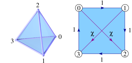
Figure 1: Species interactions represented by an oriented graph (right), the arrows indicating the invasion direction and 1 and $0\leq\chi\leq 1$ are the corresponding rates. The possible configurations, $(\rho_{0},\rho_{1},\rho_{2},\rho_{3})$, can be represented as points in a 3-simplex (left). Upon extinction of a single species the orbits are constrained to one of the faces of the tetrahedron, a 2-simplex. After a second extinction, the configurations are constrained to the line joining the two surviving species (1-simplex). If eventually a single species remains, this state is represented by the corresponding vertex.

The paper is organized as follows. Next section discusses the mean field approach for the fully mixed version of the model, in particular, the stable fixed points both for $\chi=0$ and $\chi\neq 0$. Then, we present the results for the spatially structured system, with emphasis on the long term persistence of the coexistence state. Finally, we discuss the similarities and discrepancies of both approaches and present our conclusions.

2 Analytical Results

When spatial correlations are neglected and individuals have the same probability to interact with all others, irrespective of their distance, one may attempt a mean field description. Let $\rho_{i}$ be the density of species $i$ (obviously $\sum_{i}\rho_{i}=1$). Time variations in the densities may only occur due to interactions between different species, in which the stronger one will invade the weaker with rate 1 or $\chi$. The mean field equations depend only on the frequency of such encounters and read:

$$\dot{\rho_{i}}=\sum_{j}I_{ij}\rho_{i}\rho_{j},$$ (1)

where each element of the interaction matrix, $I_{ij}$, is the rate with which species $i$ invades $j$. A negative $I_{ij}$ means that the invasion direction is reversed. The matrix ${\bm{I}}$ is given by

$${\bm{I}}=\left[\begin{array}[]{cccc}0&1&\chi&-1\\ -1&0&1&\chi\\ -\chi&-1&0&1\\ 1&-\chi&-1&0\end{array}\right].$$ (2)

These equations present several equilibrium points such that $\dot{\rho}_{i}=0,\forall i$. The linear stability of these steady states is determined by the sign of the real part of the eigenvalues of the Jacobian matrix. If at least one eigenvalue has a positive real part, the corresponding fixed point is unstable, otherwise it is stable. Furthermore, a stable equilibrium point may be asymptotically attainable when all real parts are strictly negative. When there are purely imaginary eigenvalues, the stable equilibrium is neutral and never attainable dynamically.

The fixed points for $\chi=0$ have been discussed by several authors [SaYoKo02, SzFa07, DoFr12, CaDuPlZi10, DuCaPlZi11]. First, there are four absorbing states that are heteroclinic points (saddle points) [HoSi98], at the vertices of the 3-simplex, in which only one species survives: $(1,0,0,0)$, $(0,1,0,0)$, $(0,0,1,0)$ or $(0,0,0,1)$. In addition to these, and because species 0 and 2 (or 1 and 3) are mutually neutral, any point on the line connecting each pair is also a fixed point, the initial proportion between them kept constant:

$$\left(c_{o},0,1-c_{o},0\right)$$ (3)

$$\left(0,c_{o},0,1-c_{o}\right),$$ (4)

with $0\leq c_{o}\leq 1$. Lastly, there is a coexistence fixed point in the interior of the 3-simplex, for which all densities are non zero,

$$\left(c_{o},\frac{1}{2}-c_{o},c_{o},\frac{1}{2}-c_{o}\right),$$ (5)

with $0\leq c_{o}\leq 1/2$, a particular example being the symmetric state $(1/4,1/4,1/4,1/4)$. This point is stable, but not asymptotically stable. In fact, there are two integrals of motion: $\rho_{0}\rho_{2}$ and $\rho_{1}\rho_{3}$. In contrast, for the ${\cal S}=3$ game there is only one invariant of motion: $\rho_{0}\rho_{1}\rho_{2}$.

With $\chi\neq 0$, the coexistence state Eq. (5) is no longer a solution of Eq. (1). Nonetheless, there are two further fixed points in which one species (1 or 2) dies out and the remaining three species form a non homogeneous RSP game [LiDoYa12]:

$$\left(\frac{1}{2+\chi},0,\frac{1}{2+\chi},\frac{\chi}{2+\chi}\right)$$ (6)

$$\left(\frac{\chi}{2+\chi},\frac{1}{2+\chi},0,\frac{1}{2+\chi}\right).$$ (7)

Notice that for $\chi=0$ the above fixed points are particular cases of Eqs. (3) and (4), respectively. The first solution, in which the species 1 becomes extinct, is an unstable fixed point, while the second one, in which species 2 goes extinct and the remaining three compose a heterogeneous RSP game, is (neutrally) stable. In the limit $\chi\to\infty$, the stable solution Eq. (7) becomes $(1,0,0,0)$ and species 0 dominates. An example, Fig. 2, shows the evolution from the symmetrical initial state with $\rho_{i}=1/4,\forall i$ and $\chi=0.5$. The system approaches a closed orbit that oscillates around $(0.2,0.4,0,0.4)$, Eq. (7), after the exponentially fast extinction of species 2. When $\rho_{2}=0$, the quantity $\rho_{0}^{\chi}\rho_{1}\rho_{3}$ is an integral of motion [HoSi98, IfBe03, ReMoFr06]. Interestingly, besides the trivial normalization condition, no invariant involving all four densities exists for $\chi\neq 0$. The fixed points are equivalent to the time average of the oscillating densities. Both the period of the oscillations and the time that species 2 takes to become extinct diverge when $\chi\to 0$ since in this limit the existence of the invariants of motion mentioned above precludes the possibility of an extinction. Indeed, when $\chi=0$, the homogeneous initial condition considered here becomes a fixed point with four coexisting species. For the homogeneous case, $\chi=1$, one recovers the $\rho_{i}=1/3,\forall i$, solution. Notice that each species density depends on its prey’s invasion rate and when we decrease $\chi$ (species 1 invasion rate over 3), although one would expect a decrease in its density, it is the density of its predator, species 0, instead, that decreases. This is known as the “survival of the weakest” principle [Tainaka93, FrAb01].

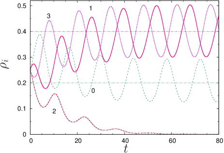
Figure 2: Example of the time evolution for $\chi=0.5$ within mean field, starting with $\rho_{i}(t=0)=1/4,\forall i$. Species 2 rapidly becomes extinct and the remaining three species oscillate, out of phase, around the respective neutrally stable fixed point (dashed lines) given by Eq. (7), $(0.2,0.4,0,0.4)$. The fixed point also corresponds to an average of $\rho_{i}$ over a period, once the stationary state is attained.

When spatial correlations are important, as when agents are placed on a lattice (see Section 3), the mean field approach usually breaks down. One of the simplest ways to go beyond the mean field predictions is to use the pair approximation (PA) [MaDi99]. Within this approach one considers the dynamics of pairs of connected sites (instead of only one-site quantities as in MF). As the corresponding equations depend on triplets of connected sites, the system is closed by choosing an ansatz relating three- and two-site quantities. For the PA the ansatz chosen is of the form $P(123)=P(12)P(23)/P(2)$, where $P(123)$ is the probability of having species 1, 2, and 3 occupying three connected sites (2 occupies the central site). $P(12)$ and $P(23)$ are similarly defined.

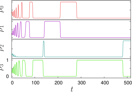
Figure 3: (Top panel) Numerical resolution of the pair approximation equations for $\chi=0.45$, starting with $\rho_{i}(t=0)=1/4,\forall i$. Notice that $\rho_{2}$ decreases to very small values during the transient, and the system approaches the 310 cycle. Later, however, $\rho_{2}$ grows once again and the system switches to the 3210 cycle. (Bottom panel) The same orbit plotted in the simplex. The black dot signals the starting point. Although initially the orbit approaches the 310 face and the species 2 seems to go extinct, it eventually resumes and the full 3210 cycle is populated (notice that the orbit goes very close to the edges of the simplex at later times).

For the system considered here the PA does not have any fixed points with coexistence of the four species. In fact, when expressed in term of species densities, the fixed points of the PA coincide with those found using MF. One important difference is that the fixed point for which there is extinction of species 2 is asymptotically unstable. As happens in the case of the RSP game [MaLe75, SzSzIz04], the model has a heteroclinic cycle involving the four species. In addition, the diagonal interactions give rise to two new heteroclinic cycles involving species 0, 1 and 3, and 0, 2 and 3. As these cycles share some nodes, none of them can be asymptotically stable. This, however, does not mean that they cannot dominate the dynamics. Solving the PA equations of motion for several different initial conditions shows that for long times the system asymptotically approaches the 3210 cycle. However, for shorter times the system moves towards the vicinity of the 310 cycle, and can stay there for a long time until it “jumps” to the vicinity of the 3210 cycle. This can be thought of as a ‘competition’ between the cycles [KiSi94] that is eventually won by the cycle 3210 (the cycle 023 does not seem to play any role in the dynamics). The fact that the density of species 2 falls to extremely low levels during the transient implies that in a stochastic version of this dynamics the extinction of species 2 would happens after a rather short time. The duration of this transient is an increasing function of $\chi$. Unfortunately, it is not possible to obtain the time average of the densities of any of the species because these quantities do not converge [Ga92]. The above behavior is illustrated in Fig. 3. In particular, notice that species 2 resumes to a noticeable density in the top panel of Fig. 3. All four densities appear on the heteroclinic orbit, one at a time (with the others being extremely small) with increasing periods of stasis on each (unstable) monoculture [MaLe75, HuWe01]. Although all four species have non zero densities, the heteroclinic cycle is termed “impermanent coexistence” [HuLa85] since they do not coexist with finite densities. In the bottom panel, on the other hand, the orbit is depicted in the simplex of Fig. 1. Initially (the starting point is the black dot) the orbit approaches the 310 face but eventually species 2, that was only apparently extinct, increases its density once again and the system stabilizes on the full 3210 heteroclinic cycle.

To summarize, the system tends to decrease the amount of hierarchy (because of the $\chi$ weighted connections) by the exponentially fast extinction of one species, converging to a fully intransitive, non hierarchical, three species system [LiDoYa12]. Indeed, in mean field, any amount of transitivity (measured by $\chi$) destroys the possible coexistence state that exists when $\chi=0$.

3 Simulations

The dynamics on a lattice may be very different from the evolution predicted by the mean field equations, mainly because the range of interaction being much smaller than the system size, local correlations play an important role. Moreover, unless the system is very large, finite size effects exist and introduce stochastic effects. As an example, the invariants discussed in the previous section, quantities that are kept constant during the motion along closed orbits, no longer persist for finite systems, and density fluctuations eventually drive the system, through extinctions, into an absorbing state. These finite size effects become less important for large systems and disappear for $L\to\infty$, where $L$ is the system linear size. In order to study the system on the lattice, we consider a square grid with $N=L^{2}$ sites with periodic boundary conditions and, with the same probability, one of the four species is randomly assigned to each of those sites at $t=0$. One site and one of its neighbors is chosen at random and the stronger site invades the other, depending on the species, with probability either unity or $\chi$. This step is repeated $N$ times, what defines the time unit. Analogous to the mean field approach, the densities oscillate in time, however, the amplitude of these oscillations seems to decrease with the size of the system and tend to disappear for very large systems.

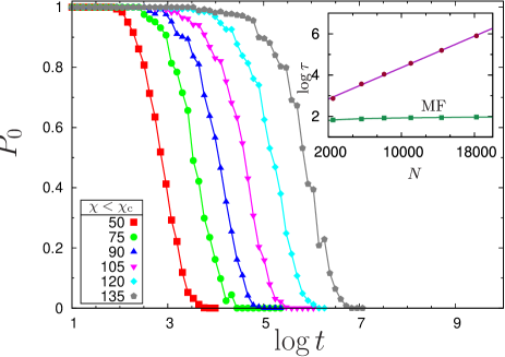
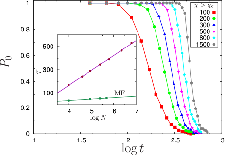
Figure 4: (Top panel) Probability of all species surviving up to time $t$, for $\chi=0.31<\chi_{\scriptstyle\rm c}$ and several linear sizes $L$. Data are averages over at least 200 samples. The characteristic extinction time $\tau$, defined as $P_{0}(\tau)\equiv 1/2$, is shown in the inset and grows exponentially with the system size. For comparison, we also show in the inset the characteristic extinction time for a finite fully mixed system (see text). (Bottom panel) The same, but for $\chi=0.5>\chi_{\scriptstyle\rm c}$. The characteristic extinction time shown in the inset has a logarithmic dependence on $N$. Notice the very different horizontal scales in the two panels.

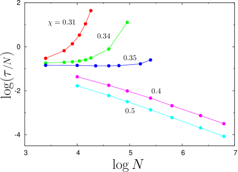
Figure 5: Average extinction time $\tau$ versus $N$ for several values of $\chi$. The critical value of $\chi$, $\chi_{\scriptstyle\rm c}$, is slightly above $\chi=0.35$. Notice the two different asymptotic behaviors, $\tau(\chi<\chi_{\scriptstyle\rm c})/N\to\infty$ and $\tau(\chi>\chi_{\scriptstyle\rm c})/N\to 0$. For $\chi\simeq\chi_{\scriptstyle\rm c}$, $\tau$ is linear in $N$. The lines are only guide to the eyes.

Even though a deterministic system may have stable coexistence states, in its stochastic counterpart the finite number of interacting agents induce fluctuations that, given enough time, eventually lead to the extinction of one or more species. However, as the system size increases, distinct dynamical behaviors may be observed depending on the value of $\chi$. The dependence of the average characteristic time for an extinction to occur on the system size $N$ allows for a classification of the possible occurrying scenarios [AnSc06, ReMoFr07a, CrReFr09b, Frey10]. The coexistence is said to be stable when the related deterministic dynamics presents a stable atractor in the coexistence phase, and this is associated with an exponentially increasing time for the first extinction to occur as $N$ increases. Analogously, the unstable state presents a logarithmic increase of the extinction time and the deterministic system approaches an absorbing state. In between, a power law dependence of the extinction time on the system size is related with the presence of closed, neutrally stable orbits in the deterministic case. The top panel of Fig. 4 shows, for small values of $\chi$ and several linear sizes $L$, the probability that the system does not suffer any extinction up to the time $t$, $P_{0}(t)$, that is, the probability of a persistent coexisting state. The larger the system is, the longer it takes for $P_{0}$ to start dropping. We may define a characteristic time for the first extinction, $\tau(N)$, as the time when $P_{0}$ drops to half its initial value, that is, $P_{0}(\tau)\equiv 1/2$. In the inset of Fig. 4, top panel, one can observe, for the range of sizes considered here, that $\tau(N)$ has an exponential growth and even for modest sizes, the time of the first extinction is very large. Extinction [OvMe10] in this case is driven by very rare fluctuations and the coexistence is said to be stable [AnSc06, ReMoFr07a, CrReFr09b, Frey10]. On the other hand, for large $\chi$, inset of Fig. 4, bottom panel, the extinction time growth is logarithmic in $N$ and even for very large systems (one order of magnitude larger than in the previous case), $\tau$ is rather small. Coexistence in this case is unstable and even small fluctuations are able to drive some species to extinction [ReMoFr07a, CrReFr09b]. Thus, comparing these two cases, there must be a dynamical critical value of $\chi$, $\chi_{\scriptstyle\rm c}$, separating those two quite distinct dynamical behaviors of $\tau(N)$, and a rough estimate places this critical value at $\chi_{\scriptstyle\rm c}\simeq 0.35$. Indeed, as shown in Figs. 4 and 5, $\tau(\chi<\chi_{\scriptstyle\rm c})$ and $\tau(\chi>\chi_{\scriptstyle\rm c})$ have very distinct asymptotic behavior [ScCl10]. While for $\chi<\chi_{\scriptstyle\rm c}$ the mean extinction time $\tau$ grows exponentially, above $\chi_{\scriptstyle\rm c}$ this growth is logarithmic in $N$. The intermediate region, for $\chi\simeq\chi_{\scriptstyle\rm c}$, the scaling of $\tau$ with the system size is polynomial. For $\chi>\chi_{\scriptstyle\rm c}$ species 2 goes extinct and the three remaining ones converge to densities close to the fixed point Eq. (7). It is also important to stress that a second extinction, when it occurs, takes a much longer timescale. Both insets of Fig. 4 also show the comparison with the correspondent $\tau$ for a finite fully mixed system. To simulate such a system, in each MC step, new neighbors are randomly assigned to each site, without any distance constraint. For both $\chi>\chi_{\scriptstyle\rm c}$ and $\chi<\chi_{\scriptstyle\rm c}$, $\tau$ grows logarithmicly with $L$, but with a small declivity, and no distinction exists between the two regions.

For $\chi<\chi_{\scriptstyle\rm c}$, due to the exponential growth of $\tau$, the coexistence state is said to be stable and large systems stay in a state in which all four species attain a non zero fixed point. The average asymptotic density $\overline{\rho}_{i}$ for large systems can be obtained by extrapolating the above behavior, that is, $\overline{\rho}_{i}=\lim_{t\to\infty}\lim_{N\to\infty}\rho_{i}(t)$ (notice that the limits are not interchangeable). The results are shown in Fig. 6 as a function of $\chi$. The dynamical transition is clearly seen as the point at which species 2 goes extinct. Notice that all four densities are different, both above and below $\chi_{\scriptstyle\rm c}$.

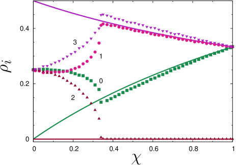
Figure 6: Stationary densities as a function of $\chi$. Although on a lattice we do not observe an oscillating behavior, there are sample to sample fluctuations and we average over at least 1000 samples (symbols). The lines are the fixed point, Eq. (7), of the mean field equations. Notice that albeit the reasonable agreement for $\chi>\chi_{\scriptstyle\rm c}$, below this value the system is in a state, not captured by the mean field approach, in which all four species coexist.

Comparing with the mean field predictions, we notice several fundamental differences. First of all, the coexistence state only appears on the regular lattice since for $\chi\neq 0$, in mean field, species 2 always gets extinct. Thus, the dynamical transition that we observe does not exist for a fully mixed system. Indeed, we can simulate the system with annealed neighbors, and the characteristic time of the first extinction is small, presenting a logarithmic growth with $N$ for all $\chi$, as can be seen in both insets of Fig. 4. The second difference is that although oscillations are observed for finite systems, they tend to disappear for very large sizes [LaSc09]. A possible explanation is that for a sufficiently large system, several different regions will evolve almost independently with uncorrelated phases, such that the overall system no longer presents oscillations. The third difference is that while the mean field behavior is monotonous on $\chi$ ($\overline{\rho}_{2}$ is always zero, $\overline{\rho}_{0}$ is always increasing and $\overline{\rho}_{1}=\overline{\rho}_{3}$ is always decreasing), on the regular lattice the behavior is non monotonous, Fig. 6. Species 1 and 3 densities, now resolved, increase for $\chi$ up to $\chi_{\scriptstyle\rm c}$ and decrease afterwards (species 0 has the opposite behavior). Notice, however, that although above $\chi_{\scriptstyle\rm c}$ the agreement with mean field is reasonable, below $\chi_{\scriptstyle\rm c}$ there is both qualitative and quantitative disagreement. In particular, all four densities are different and no fixed point predicted by the mean field approach has such a property for $\chi\neq 0$.

4 Conclusions

We studied a minimal model for a trophic network presenting multiple loops of interacting species, focusing on the effects of a tunable transitivity on the persistence of the coexistence state. As the invasion rate $\chi$ is changed, we observed two distinct dynamical phases separated by a transition at $\chi_{\scriptstyle\rm c}\simeq 0.35$, one for $\chi<\chi_{\scriptstyle\rm c}$ in which the coexistence state is stable (the mean extinction time exponentially grows with the size of the system) and the other for $\chi>\chi_{\scriptstyle\rm c}$ in which one species goes extinct on logarithmic timescales and the system ends up performing a heterogeneous RSP game. At the transition region between those two regimes, $\chi\simeq\chi_{\scriptstyle\rm c}$, $\tau$ presents a polynomial scaling with the size of the system. This transition, and the coexistence state observed in the simulations are not captured by the mean field approach.

For $\chi=0$, each species around the external four species loop has one prey and one predator. In addition, for $\chi\neq 0$ there are four internal loops with three species, two intransitive (013 and 023) and two transitive (012 and 123). In this case, because of the even number of species, the number of predators and preys of each species may differ. Thus, depending on the arrows orientation, there are three possible choices for the number of preys (or, equivalently, predators): $(3,2,1,0)$, $(3,1,1,1)$ and $(2,2,1,1)$. We only considered the last structure, Fig. 1, that is somewhat intermediate between an intransitive and a hierarchical system. The larger is $\chi$, the less intransitive the system is and one can expect that the amount of coexistence will decrease. However, we have shown that under the presence of spatial correlations and a not too large transitivity, this system may persist in a state of full diversity over exponentially large timescales. For larger levels of transitivity, on the other hand, the system eventually evolves into a three species hierarchical system, irrespective of the spatial structure [LiDoYa12]. We thus observe a dynamical transition between these two regimes on the spatially structured system, at $\chi_{\scriptstyle\rm c}$, not captured by a mean field analysis. Notice that any extinction drives the system into an absorbing state and diversity, due to the absence of mutations, is an always decreasing quantity for this class of model. Below $\chi_{\scriptstyle\rm c}$, mean field is not a good approximation for the lattice dynamics of our system either quantitatively or qualitatively. The threshold value of $\chi$ also indicates that above a certain level of intransitivity ($\chi>\chi_{\scriptstyle\rm c}$), spatial correlations are no longer important and the system on a lattice is attracted to the mean field fixed points (the densities are non oscillating). Even though the pair approximation is assumed to be a better approximation than mean field, in our case it does not provide a better description of the dynamics, in terms of fixed points. For short times the dynamics of the PA does look similar to the mean field dynamics, since for large values of $\chi$ the density of species 2 drops to extremely low values, but for longer times the dynamics is dominated by a heteroclinic cycle involving all four species.

Non monotonous responses driven by the spatial correlations are observed, while the mean field approach predicts a monotonous behavior as $\chi$ changes. For $\chi<\chi_{\scriptstyle\rm c}$, species 2 and 3 (and, analogously, 0 and 1) respond in opposite ways: while $\overline{\rho}_{3}$ increases with $\chi$, $\overline{\rho}_{2}$ decreases. The opposite behavior was predicted in the mean field approach. On the other hand, above $\chi_{c}$ the trends agree with the mean field prediction. Interestingly, in spite of presenting opposite behavior when $\chi$ increases, species 0 and 1 both become more aggressive. Since both predate on 2, this species has the smallest density (and becomes extinct in mean field). For $\chi>\chi_{\scriptstyle\rm c}$, $\overline{\rho}_{2}=0$ and the remaining three species form a heterogeneous RSP game that obeys, both on the lattice and in MF, the usual “survival of the weakest” principle: as the invasion rate $\chi$ of the weakest species (1) increases, its density $\overline{\rho}_{1}$ decreases, while the density of “the prey of the prey of the weakest” [DuCaPlZi11], in this case species 0, increases. For $\chi<\chi_{\scriptstyle\rm c}$, since all four species survive, the “the prey of the prey of the weakest” principle [DuCaPlZi11] must be modified because some species have multiple preys. Although species 0 and 1 have a wider range of possible targets, they are less efficient since their overall success rate is less than 1 ($1+\chi\leq 2$), and may be considered the weakest species. Species 2 and 3, on the other hand, fully overtake their preys. Nonetheless, the prey of the two weakest (species 2), itself stronger than them, goes extinct. Thus, although there is no obvious generalization of the above principle, one notice that the ambiguity in defining strong and weak in this case may be raised by allowing all six parameters to be different, what may, in turn, allow for such an statement. It is also clear that statements like this will become more intricate as the number of species increases.

Further questions arise for such systems. For example, in order to better understand the effects of different levels of transitivity, in particular to probe anomalous responses as the “survival of the weakest”, the study of other trophic structures with four species, and larger values of ${\cal S}$ as well, is important. In addition, finite populations may have a different behavior. Indeed, the community size, besides setting the scale for the average extinction time, may also influence which is the surviving species [MuGa10]. One may also probe the robustness of the results presented here, for example, by studying different lattices (random graph, small world, etc), dimensions and initial conditions. On a regular lattice, geometric and dynamical properties of the evolving groups are also of interest [AvBaLoMe12, AvBaLoMeOl12]. How to properly quantify the transitivity of a trophic network and correlate it with the coexistence present in a population is still an open problem (e.g., [Petraitis79, LaSc06, LaSc08, LaSc09, RoAl11, ShMc12] and references therein). We have shown that the structure alone is not enough to predict whether there will be coexistence or not. Considering the trophic relations as a weighted network may lead to an index allowing different levels of coexistence based on the same structure. Finally, allowing general weights on the trophic network [DuCaPlZi11] shall present an even richer behavior in the presence of crossed interactions.