PageRank of integers

Abstract

We build up a directed network tracing links from a given integer to its divisors and analyze the properties of the Google matrix of this network. The PageRank vector of this matrix is computed numerically and it is shown that its probability is inversely proportional to the PageRank index thus being similar to the Zipf law and the dependence established for the World Wide Web. The spectrum of the Google matrix of integers is characterized by a large gap and a relatively small number of nonzero eigenvalues. A simple semi-analytical expression for the PageRank of integers is derived that allows to find this vector for matrices of billion size. This network provides a new PageRank order of integers.

1 Introduction

The number theory [1] is the fundamental branch of mathematics where the theory of prime numbers, besides its beauty, finds important cryptographic applications [2]. It is established that the methods of the Random Matrix theory and quantum chaos find their useful applications for the understanding of properties of prime numbers and the Riemann zeros [3, 4, 5].

In this work we propose another matrix approach to the number theory based on the Markov chains [6] and the Google matrix [7]. The later finds important applications for the information retrieval and Google search engine of the World Wide Web (WWW) [8]. The right eigenvector of the Google matrix with the largest eigenvalue is known as the PageRank vector. The elements of this vector are non-negative and have the meaning of probability to find a random surfer on the network nodes. The PageRank algorithm ranks all websites in a decreasing order of components of the PageRank vector (see e.g. detailed description at [8]). Here, we propose a natural way to construct the Google matrix of positive integers using their division properties. We study the statistical properties of the PageRank vector of this matrix and discuss the properties of a new order of integers given by this ranking. The properties of the eigenvalues and eigenvectors are also discussed.

The paper is constructed as follows: in Section 2 we give the definition of the Google matrix of integers, the properties of its PageRank vector are analyzed in Section 3, the analysis of spectral properties is given in Section 4, the analytical expressions for the PageRank vector are presented in Sections 4,5 and the discussion of the results is presented in Section 6.

2 Google matrix of integers

The elements of the Google matrix $G(\alpha)$ of a directed network with $N$ nodes are given by

$$G_{mn}(\alpha)=\alpha S_{mn}+(1-\alpha)/N\;\;.$$ (1)

Here the matrix $S$ is obtained by normalizing to unity all columns of the adjacency matrix $A_{mn}$, and replacing the elements of columns with only zero elements, corresponding to dangling nodes, by $1/N$. An element $A_{mn}$ of the adjacency matrix is equal to unity if a node $n$ points to node $m$ and zero otherwise. The damping parameter $\alpha$ in the WWW context describes the probability $(1-\alpha)$ to jump to any node for a random surfer. The value $\alpha=0.85$ gives a good classification of pages for WWW [8]. The matrix $G$ belongs to the class of Perron-Frobenius operators [8], its largest eigenvalue is $\lambda=1$ and the other eigenvalues obey $|\lambda|\leq\alpha$. In typical WWW networks the eigenvalue $\lambda=1$ is strongly degenerate at $\alpha=1$ (see e.g. [9]) and the introduction of $\alpha<1$ becomes compulsory to define a unique right eigenvector at $\lambda=1$ and to ensure the convergence of the PageRank vector by the power iteration method [8]. The right eigenvector at $\lambda=1$ gives the probability $P(n)$ to find a random surfer at site $n$ and is called the PageRank. Once the PageRank is found, all nodes can be sorted by decreasing probabilities $P(n)$ and an increasing index $K(n)$. The node rank is then given by index $K(n)$ which reflects the relevance of the node corresponding to a positive integer $n$. The PageRank dependence on $K$ is well described by a power law $P(K)\propto 1/K^{\beta_{in}}$ with $\beta_{in}\approx 0.9$. This is consistent with the relation $\beta_{in}=1/(\mu_{in}-1)$ corresponding to the average proportionality of PageRank probability $P(n)$ to its in-degree distribution $w_{in}(k)\propto 1/k^{\mu_{in}}$ where $k(n)$ is a number of ingoing links for a node $n$ [8]. For the WWW it is established that for the ingoing links $\mu_{in}\approx 2.1$ (with $\beta_{in}\approx 0.9$) while for out-degree distribution $w_{out}$ of outgoing links a power law has the exponent $\mu_{out}\approx 2.7$ [10, 11]. Here we analyze properties of PageRank and use the notation $\beta=\beta_{in}$.

• 

Figure 1: The Google matrix of integers: the amplitudes of the matrix elements $G_{mn}$ at $\alpha=1$ are shown by color with blue for minimal zero elements and red for maximal unity elements, with $1\leq n\leq N$ corresponding to $x-$axis (with $n=1$ corresponding to the left column) and $1\leq m\leq N$ for $y-$axis (with $m=1$ corresponding to the upper row). The matrix sizes are $N=31$ in the left panel and $N=101$ in the right panel.

To construct the Google matrix of integers, we define for $m,n\in\{1,\,\ldots,\,N\}$ the adjacency matrix by $A_{mn}=k$ where the $k$ is a “multiplicity” defined $k$ as the largest integer such that $m^{k}$ is a divisor of $n$ and if $1<m<n$, and $k=0$ if $m=1$ or $m=n$ or if $m$ is not a divisor of $n$. Thus we have $k=0$ if $m$ is not a divisor of $n$ and $k\geq 1$ if $m$ is a divisor of $n$ different from $1$ and $n$. The total size $N$ of the matrix is fixed by the maximal considered integer.

This defines a network where an integer number $n$ is linked to its divisors $m$ different from $1$ and $n$ itself and where the transition probability is proportional to the multiplicity $k$, the number of times we can divide $n$ by $m$. The number $1$ and the prime numbers are therefore not linked to any other number and correspond to dangling nodes in the language of WWW networks. For example, the number $n=24$ has links pointing to $m(k)=2(3),\,3(1),\,4(1),\,6(1),\,8(1),\,12(1)$ (multiplicity is given in the brackets) so that the nonzero matrix elements in this column are $3/8,\,1/8,\,1/8,\,1/8,\,1/8,\,1/8$ respectively. We find the total number of links $N_{\ell}=\sum_{mn}A_{mn}$, taking into account the multiplicity, to be $N_{\ell}=6005$ at $N=1000$, $N_{\ell}=1066221$ at $N=10^{5}$, $N_{\ell}=152720474$ at $N=10^{7}$, $N_{\ell}=19877650264$ at $N=10^{9}$. The fit of the dependence $N_{\ell}=N\,(a_{\ell}+b_{\ell}\ln N$) gives $a_{\ell}=-0.901\pm 0.018$, $b_{\ell}=1.003\pm 0.001$.

From the adjacency matrix $A$ we first construct a matrix $S_{0}$ by normalizing the sum in each column, containing at least one non-zero element, to unity and the matrix $S$ is obtained from $S_{0}$ by replacing the elements of columns with only zero elements, corresponding to dangling nodes 1 and prime numbers, by $1/N$. The Google matrix $G$ is finally obtained from $S$ by Eq. (1) for an arbitrary damping factor. The PageRank is the right eigenvector of the matrix $G$ with the maximal eigenvalue $\lambda=1$: $GP=\lambda P=P$.

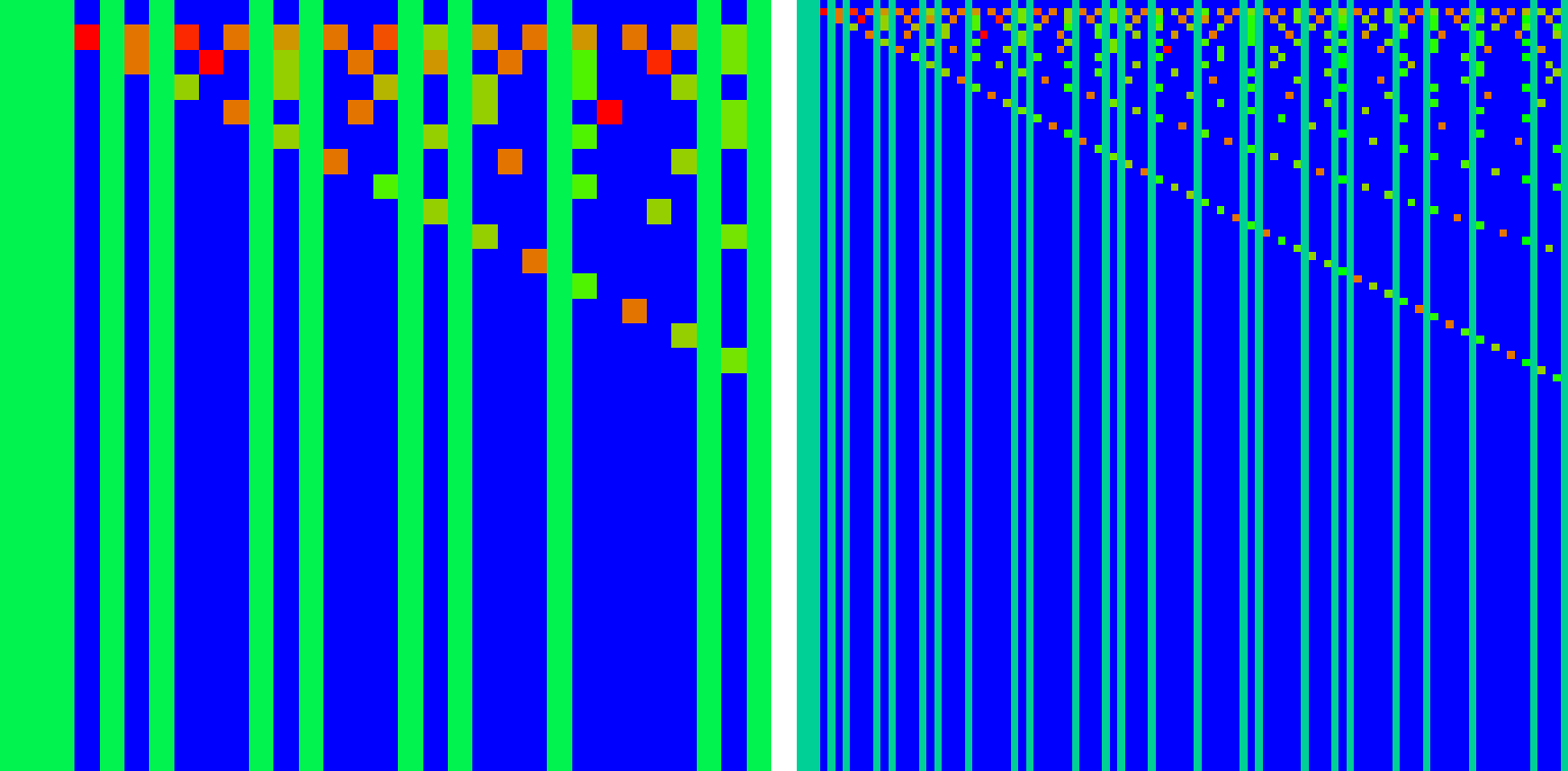
The examples of the Google matrix $G$ at $\alpha=1$ for $N=31,\,101$ are shown in Fig. 1. We see that most elements are concentrated above the main matrix diagonal since the divisors $m$ are smaller than the number $n$ itself. The only exceptions are given by the columns at $1$ and the prime numbers $p$ which have no divisors (apart from $1$ and $p$) and hence they correspond to the dangling nodes with no direct links pointing to them. The amplitude of the elements in these columns is uniformly $1/N$. The structure of the matrix clearly shows the presence of diagonals $m=n/2,\,n/3,\,\ldots$ corresponding to the small divisors $m^{\prime}=2,\,3,\,\ldots$, which appear rather often in the division of integers. This structure is preserved up to the largest size $N=10^{9}$ considered in this work.

As we will see in Section 4, the eigenvalue $\lambda_{0}=1$ of the matrix $S$ is non-degenerate (contrary to typical realistic WWW networks [9]) and in addition its spectrum has a large gap with $\lambda_{0}$ and the other eigenvalues $|\lambda_{i}|<0.6$. In such a case the PageRank vector $P(K)$ has a very small variation when the damping factor $\alpha$ is changed in the range $0.85\leq\alpha\leq 1$ and the convergence of the power method to calculate the PageRank is well assured, actually quite fast, even for the damping parameter $\alpha=1$. Therefore, we limit in this work our studies to the case $\alpha=1$ at which $G$ coincides with the matrix $S$ and from now on we denote $S$ as “the Google matrix”.

3 PageRank order of integers

We first determine the PageRank vector of the Google matrix numerically by the power iteration method [8] or by the Arnoldi method [12] using an Arnoldi dimension of size $n_{A}$, which allows to find several eigenvalues and eigenvectors with largest $|\lambda|$ for a full matrix size of a few millions (see more details in [9, 13]).

• 

Figure 2: Dependence of PageRank probability $P(K)$ on PageRank index $K$ for the matrix sizes $N=10^{3}$, $10^{4}$, $10^{5}$, $10^{6}$, $10^{7}$; the dashed straight line shows the Zipf law dependence $P\sim 1/K$.

• 

Figure 3: Dependence of PageRank probability $P$ on the integer number $n$ for matrix sizes $N=10^{6},10^{7}$ (left panel green and red points respectively), and rescaled probability $nP$ on $n$ (right panel); data are shown in log-log scale.

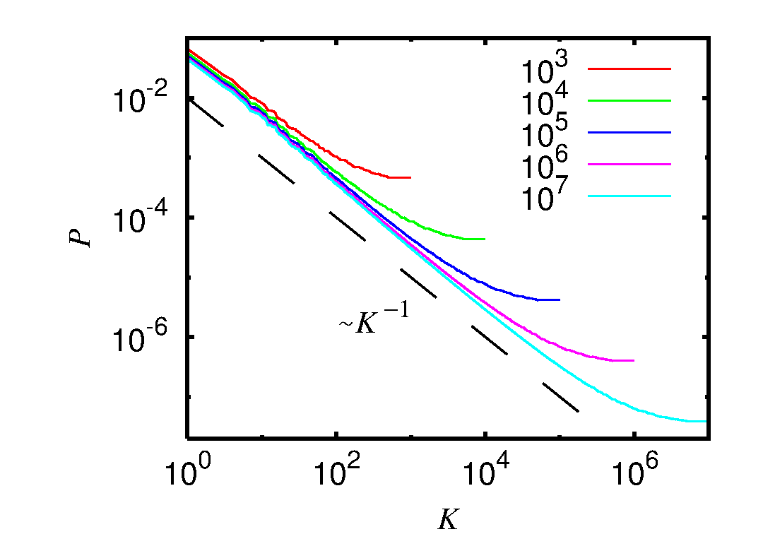
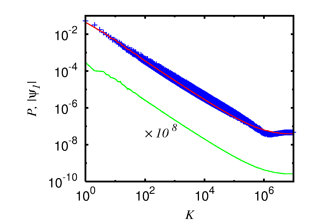
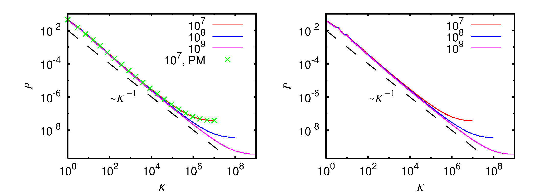
The dependence of PageRank probability $P(K)$ on PageRank index $K$ is shown in Fig. 2. We see that with the growth of the system size $N$ the dependence $P(K)$ converges to a fixed distribution $P(K)$ on initial $K\leq N/10$ values with the tail of distribution $P(K)$ at $K>N/10$ which is sensitive to the cut-off at the finite matrix size $N$. In the convergent part a formal fit (for $10<K<10^{5}$) gives the dependence $P\sim A/K^{\beta}$ with $\ln A=0.0431\pm 0.00049$, $\beta=1.040\pm 0.0015$ being close to the Zipf law with $\beta=1$ [14]. The small value of $\beta-1$ indicates that there can be a logarithmic correction. Indeed, the fit $1/(PK)=a_{1}+b_{1}\ln K$ (for $10<K<10^{3}$) gives the values $a_{1}=16.050\pm 0.187$, $b_{1}=2.468\pm 0.036$. Thus, it is possible that in the limit of $N\rightarrow\infty$ we have the asymptotic behavior $P\sim 1/(K\ln K)$. Such a scaling looks to be more probable due to usual logarithmic corrections in the density of primes [2]. However, for the available finite matrix sizes the regime of linear bevahior of $1/(PK)$ versus $\ln K$ is quite limited and it is not obvious to distinguish between the above two fitting dependencies.

• 

Figure 4: Dependence of the integer number $n$ on the PageRank index $K$ for sizes $N=10^{5},10^{6}$ (left panel green and red points respectively), and $10^{7}$ (right panel); data are shown in log-log scale.

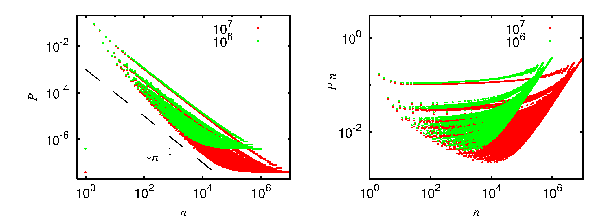
The dependence of PageRank probability $P$ on integer index $n$ is shown in Fig. 3. It is characterized by a global decay $P\propto 1/n$ with the presence of various branches which are especially well visible for the rescaled quantity $nP$. This structure is preserved with the increase of matrix size for the values of $n<N/100$. The direct check shows that the highest plateau corresponds to the prime numbers $p$.

• 

Figure 5: Top panels: dependence of the integer number $n$ on PageRank index $K$ for size $N=10^{7}$ shown by red points (left panel), right panel shows zoom of data in a rectangle from left panel. Bottom panels: in addition to data of top right panel data for $N=10^{6}$ are shown (left panel), right panel shows zoom of data in a rectangular region from left panel. Data are shown in usual scale.

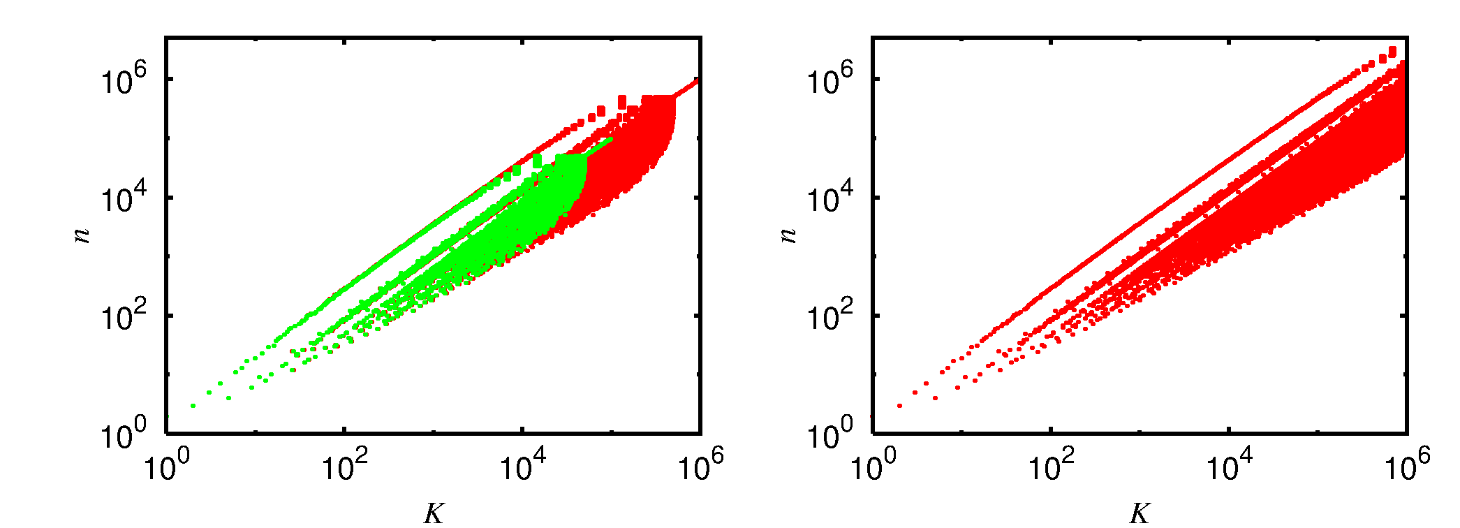
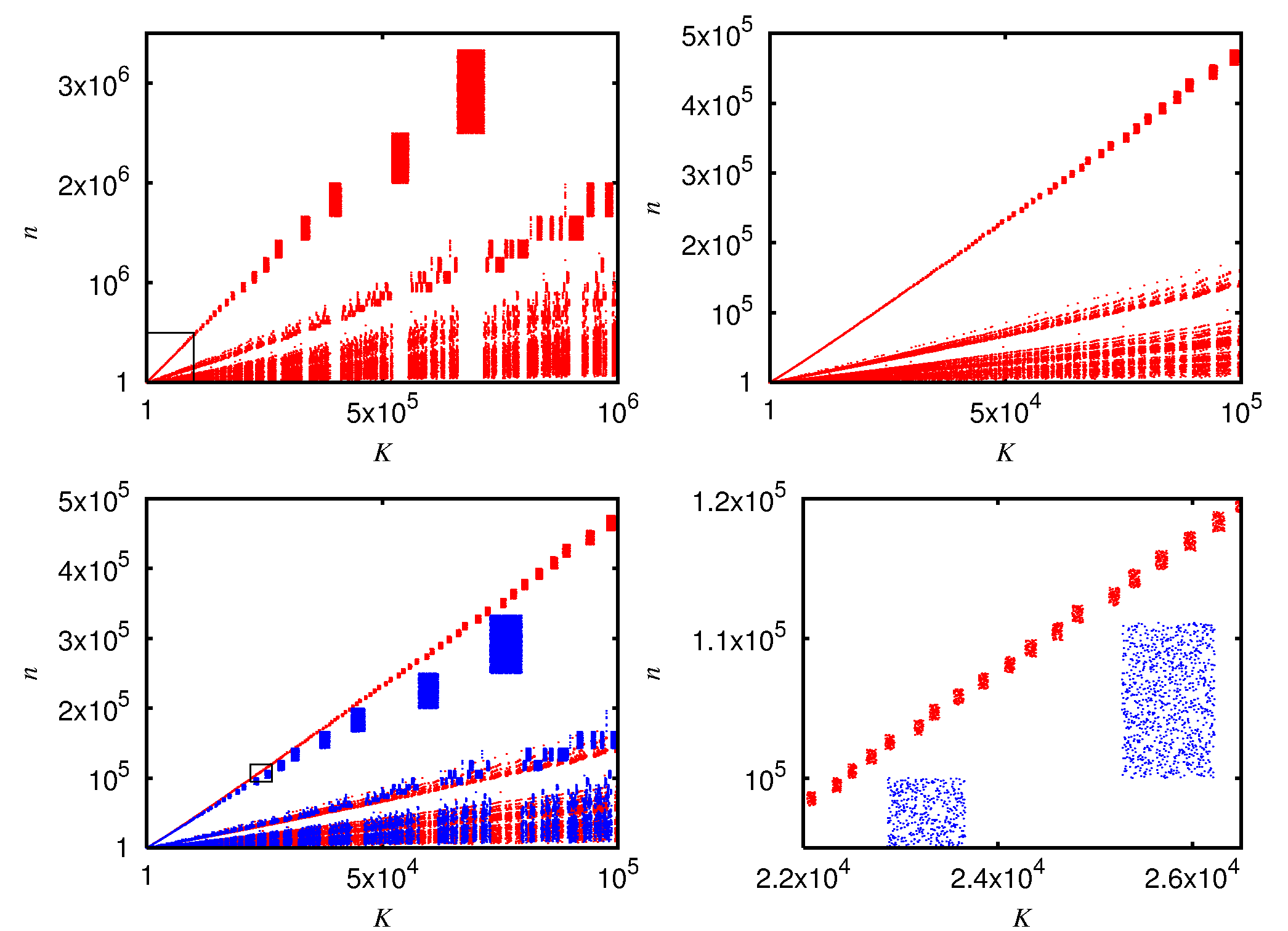
Another way to analyze the structures visible in Fig. 3 is to consider the dependence of $n$ on the PageRank index $K$ obtained from the PageRank probability $P(K_{n})$. In fact $K$ gives a new order of integers imposed by the PageRank. The dependence $n(K)$ is shown in Fig. 4 on a large scale. In a first approximation we find the layered structure with a sequence of parallel lines $n\propto K$. This global structure is preserved with the increase of the matrix size from $N=10^{5}$ to $10^{7}$.

A more detailed view of this structure is shown in Fig. 5. There are well defined separated branches with approximately linear dependence $n\approx\kappa K$ with $\kappa\approx 4.5$ for the highest branch which corresponds to the highest plateau in Fig. 3 (right panel). This branch contains only primes. The lower branch contains semi-primes (product of two primes) and so on down to smaller an smaller values of $\kappa$. The whole structure looks to have a self-similar structure as it shows a zoom to a smaller scale. The increase of the size $N$ gives some modifications of the structure keeping its global pattern (see Fig. 5 bottom panels). There is a certain clustering on the $(n,K)$ plane of rectangles containing close values of $K$ and integer numbers $n$. The rectanglers in the upper prime-branch contain exclusively prime numbers for $n=p$. Note that the neighboring non-prime values appear in other rectanglers on the right side for larger values of $K$. For example, in the bottom left panel of Fig. 5 we have a rectangle at $K\sim 2.6\times 10^{4}$ and $n\sim 10^{5}$ with primes but there is at $K\sim 7\times 10^{4}$ another rectangle of semi-primes, also with values $n\sim 10^{5}$.

The direct analysis shows that the rectangles correspond to flat plateaux with degenerate values of $P(K_{n})$ which appear for finite matrix size $N$. This degeneracy results from only rational numbers appearing in the elements of the Google matrix and from its very sparse structure. Inside such flat regions the ordering in $K$ is somewhat arbitrary and depends on the precise sorting algorithm used. The $K$ index shown in Fig. 5 was obtained by the Shellsort method that may indeed produce a quite random ordering for degenerate values thus generating the rectanglers seen in Fig. 5. We have verified that when using a modified sorting algorithm with a secondary criterium, to sort with increasing $n$ inside a degenerate region, the rectangles are replaced by lines from the left bottom corner to the right top corner. With increasing values of $N$ these rectangles are reduced in size. We numerically find that the first degenerate plateau appears at $K=K_{d}$ and that this number increases with the matrix size $N$, e.g. $K_{d}=27$ at $N=1000$, $177$ at $10^{5}$, $1287$ at $10^{7}$, $10386$ at $10^{9}$. This dependence is well described by the fit $K_{d}=a_{d}K^{b_{d}}$ with $a_{d}=1.284\pm 0.078$, $b_{d}=0.432\pm 0.004$. We return to the discussion of the convergence at large $N$ a bit later.

• 

Figure 6: Dependence of the ratio $n/K$ on the PageRank index $K$ for size $N=10^{7}$; data are shown in semi-log scale. The straight line shows the fit dependence $n/K=a_{2}+b_{2}\ln K$ for the upper branch in the range $10\leq K\leq 10^{4}$ with $a_{2}=1.3583\pm 0.0099$, $b_{2}=0.3227\pm 0.0014$.

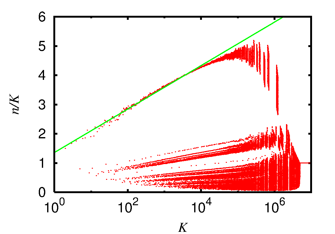
Since we find an approximate linear growth of $n$ with $K$ inside each branch it is useful to consider the dependence of the ratio $n/K$ on $K$ which is shown in Fig. 6. The upper branch of primes is well described by the dependence $n/K=0.322\ln K+1.358$ that shows that in the previous relation $\kappa$ is not a constant but grows logarithmically with $K$. We have an approximate relation $b_{2}=0.322\approx 1/b_{1}=1/2.468$. The lower branches also have an approximately logarithmic growth of the ratio $n/K$ with $K$.

• 

Figure 7: Dependence of $|\Delta K|=|K_{n}(N_{2})-K_{n}(N_{1})|$ on the integer $n$ for matrix sizes $N_{1}=10^{6},N_{2}=10^{7}$ (green points) and $N_{1}=10^{5},N_{2}=10^{6}$ (red points). Left and right panels show the same data either in normal or in log-log scales.

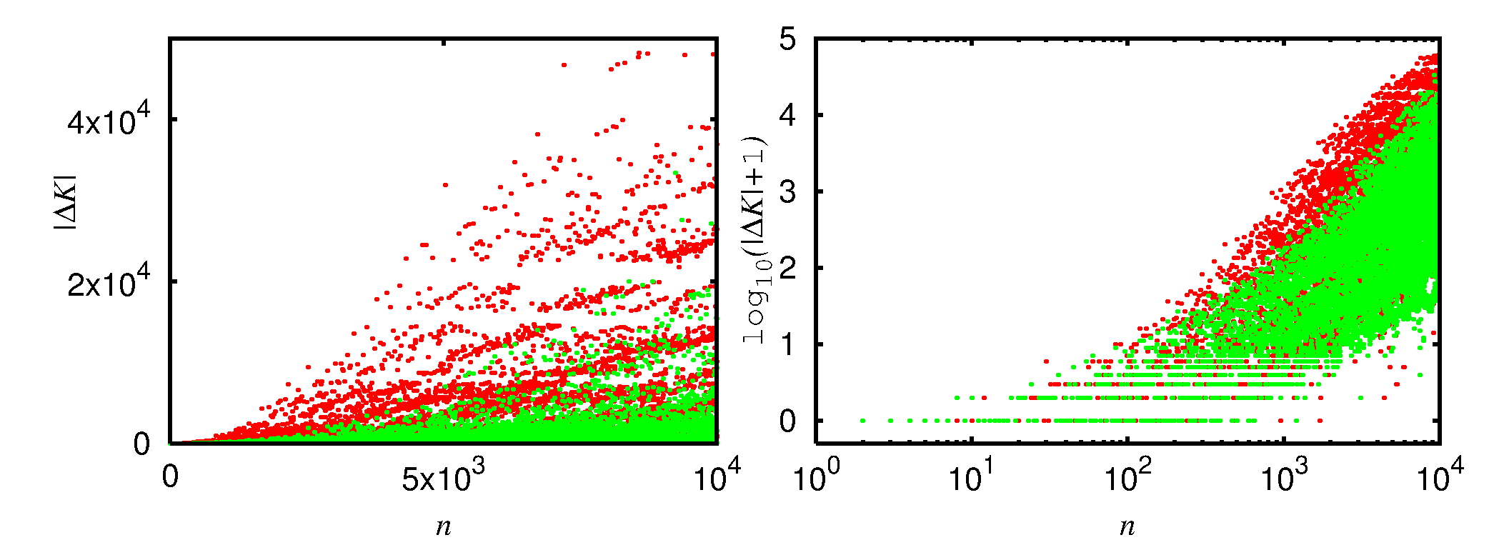
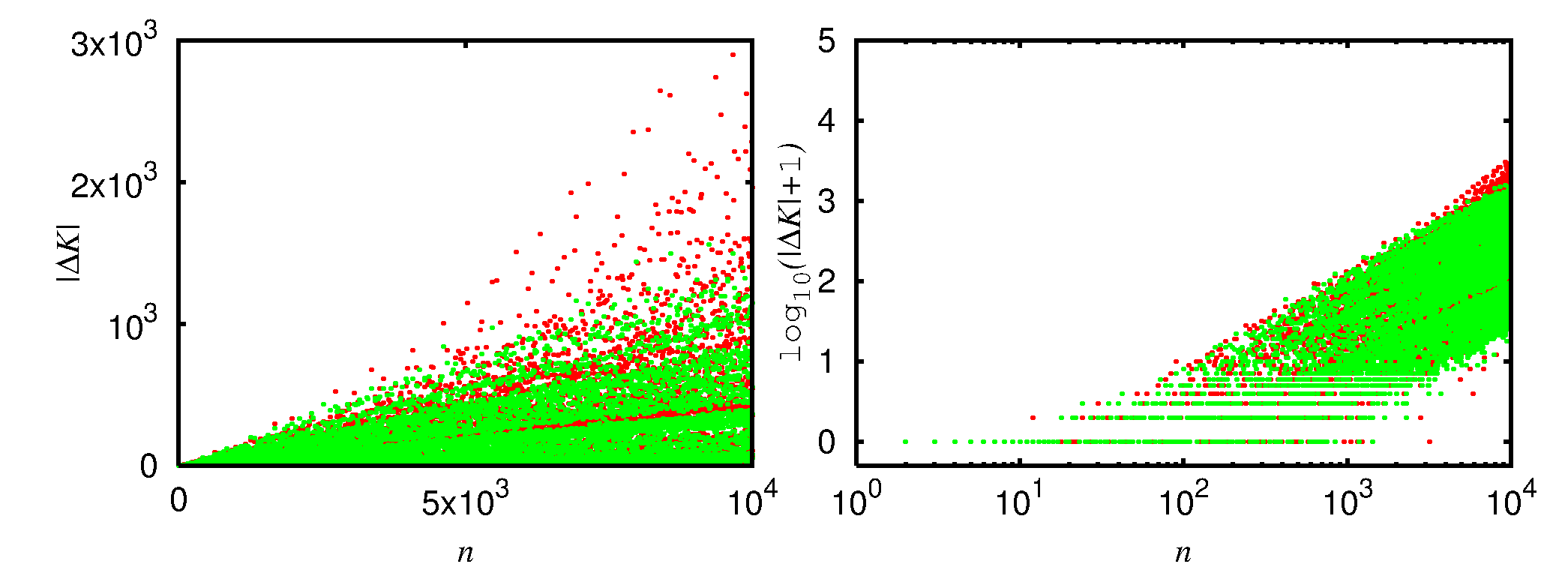
Finally, let us discuss the stability of the PageRank order of integers in respect to the variation of the matrix size $N$. The dependence $P(K)$ is definitely converging to a fixed function for $K\ll N$ as it is well seen in Fig. 2. However, for a fixed integer $n$ its PageRank index $K_{n}$ has a visible variation with the increase of matrix size $N$. These variations are visible in Fig. 5 (bottom panels). At the same time the global structure of the $K_{n}$ or $n(K)$ dependence shows signs of convergence with the growth of $N$. A more detailed analysis of variation of $\Delta K=|K_{n}(N_{1})-K_{n}(N_{2})|$ for two matrix sizes $N_{2}=10N_{1}$ is shown in Fig. 7. We see that there is a significant decrease of variations $\Delta K$ with increase of $N_{1}$, even if a small changes of $K_{n}$ values are visible even at relatively low $n\sim 100$. On the basis of these data we make a conjecture that in the limit of $N\rightarrow\infty$ we will have a convergence to a fixed PageRank order of integers $K_{n}$. However, we expect that this convergence is very slow, probably logarithmic in $N$, thus being the reason that even at $N=10^{7}$ we find some variations in $K_{n}$. We note that the density of states of Riemann zeros also shows very slow convergence so that enormously large values of $n\sim N\sim 10^{20}$ are required to obtain stable results [3, 4].

4 Spectral properties of the Google matrix of integers

4.1 Arnoldi method

To study numerically the spectrum of the Google matrix $S=G$ of integers at $\alpha=1$ we first employ the Arnoldi method [12, 13]. This method uses a normalized initial vector $\xi_{0}$ and generates a Krylov space by the vectors $S^{j}\,\xi_{0}$ for $j=0,\,\ldots,\,n_{A}-1$ where $n_{A}$ is called the Arnoldi dimension. Using Gram-Schmidt orthogonalization one determines an orthogonal basis of the Krylov space and the matrix representation of $S$ in this basis. This provides a matrix $\bar{S}$ of modest dimension $n_{A}$ of Hessenberg form which can be diagonalized by standard QR-methods and whose eigenvalues, called Ritz eigenvalues, are in general very accurate approximations of the largest eigenvalues of the original (very large) matrix $S$.

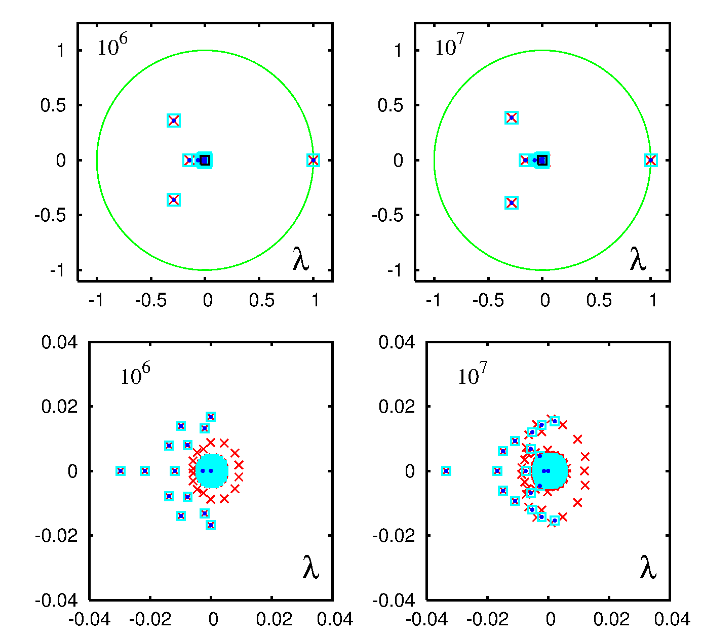
In this work we have used the Arnoldi dimension $n_{A}=1000$ and two different initial vectors, first a random initial vector and second a uniform initial vector with identical components $1/\sqrt{N}$ (thus normalized by the Euclidean norm $\|(\cdots)\|_{2}$). The spectrum of the matrix $S$ is shown in Fig. 8 for two sizes $N=10^{6},\,10^{7}$. We see that there are only three eigenvalues within the ring $0.05<|\lambda|<0.5$ while the majority of eigenvalues is concentrated inside a range of $|\lambda|<0.05$. The first few largest eigenvalues are accurately obtained from both initial vectors used for the Arnoldi method and also coincide (up to numerical precision) with the eigenvalues determined by a semi-analytical approach (see below). However for the range $|\lambda|<0.05$ the situation becomes more subtle as it is discussed below.

We note that Fig. 8 shows a large gap between $\lambda_{0}=1$ and the next eigenvalue thus justifying our above choice of the damping factor $\alpha=1$ .

• 

Figure 8: Spectrum of the Google matrix of integers for the matrix size $N=10^{6}$ (left panels) and $10^{7}$ (right panels); the red crosses (light blue squares) are numerical data from the Arnoldi method with Arnoldi dimension $n_{A}=1000$ and a random initial vector (with the unit initial vector) and the dark blue points are the exact eigenvalues obtained as the zeros of the reduced polynomial of Eq. (6). Top panels show the whole spectrum and the bottom panels show a zoom of the region represented by black squares in the top panels. The eigenvalues have significantly higher accuracy for the Arnoldi method with unit initial vector. The unit circle $|\lambda|=1$ is shown in green.

4.2 Analytical discussion of spectrum

The Google matrix $S$ at $\alpha=1$ has a very particular structure which allows to establish some important properties for the spectrum and its eigenvalues. We can write

$$S=S_{0}+v\,d^{\,T}$$ (2)

where $v$ and $d$ are two vectors of size $N$ with components $v_{n}=1/N$ and $d_{n}=1$ for prime numbers $n=p$ or $n=1$ and $d_{n}=0$ for the other non-prime numbers (different from 1). For later use we also introduce the vector $e$ with components $e_{n}=1$ and therefore $v=e/N$. In addition $d^{\,T}$ denotes the transposed line vector of $d$. The matrix $S_{0}$ is the contribution that arises from the adjacency matrix $A$ by normalizing the non-vanishing columns of the latter and the tensor product $v\,d^{\,T}$ represents the values $1/N$ which are put in the zero columns of $S_{0}$ when constructing the full matrix $S$. The normalization condition of the non-vanishing columns of $S_{0}$ can formally be written as $e^{\,T}\,S_{0}=e^{\,T}-d^{\,T}$ which is just the line vector with components $0$ for vanishing columns of $S_{0}$ (for prime numbers $n$ or $n=1$) and $1$ non-vanishing columns of $S_{0}$ (for the other non-prime numbers different from $1$). This expression provides the useful identity :

$$d^{\,T}=e^{\,T}({\leavevmode\hbox{\small 1\kern-3.55pt\normalsize 1}}-S_{0})\ .$$ (3)

Furthermore we observe that the matrix $S_{0}$ has a triagonal form with vanishing entries on the diagonals because $(S_{0})_{mn}\neq 0$ only if $m$ is a divisor of $n$ different from $1$ and $n$ and therefore for any non-vanishing matrix element $(S_{0})_{mn}$ we have $m\leq n/2<n$. This matrix structure can also be seen in Fig. 1. As a consequence $S_{0}$ is nilpotent with $S_{0}^{l}=0$ for some integer $l$. In the following let us assume that $l$ is the minimal number such that $S_{0}^{l}=0$. Obviously in our model $l=[\log_{2}(N)]$ is actually a very modest number as compared to the full matrix size $N$.

We now discuss how the form of Eq. (2) affects the eigenvalues of the full matrix $S$. Let $\psi$ be a right eigenvector of $S$ and $\lambda$ its eigenvalue :

$$\lambda\psi=S\psi=S_{0}\psi+C\,v\quad,\quad C=d^{\,T}\,\psi=\sum_{n\ {\rm prime\ or}\ n=1}^{N}\psi_{n}\quad.$$ (4)

If $C=0$ we find that $\psi$ is an eigenvector of $S_{0}$. Then $\lambda=0$ since the matrix $S_{0}$ is nilpotent and cannot have non-vanishing eigenvalues. The matrix $S_{0}$ is actually non-diagonalisable and can only be transformed to a Jordan form with quite large Jordan blocks and $0$ as diagonal element of each of the Jordan blocks.

Suppose now that $C\neq 0$ implying that $\lambda\neq 0$ since the equation $S_{0}\psi=-C\,v$ does not have a solution for $\psi$ because $S_{0}$ has many zero rows and $v_{n}=1/N\neq 0$ for each $n=1,\ldots,N$. Since $\lambda\neq 0$ the triagonal matrix $\lambda{\leavevmode\hbox{\small 1\kern-3.55pt\normalsize 1}}-S_{0}$ is invertible and from Eq. (4) we obtain :

$$\psi=C\,(\lambda{\leavevmode\hbox{\small 1\kern-3.55pt\normalsize 1}}-S_{0})^{-1}\,v=\frac{C}{\lambda}\,\sum_{j=0}^{l-1}\left(\frac{S_{0}}{\lambda}\right)^{j}\,v\quad.$$ (5)

Note that the sum is finite since $S_{0}^{l}=0$. The eigenvalue $\lambda$ is determined by the condition that this expression of $\psi$ has to satisfy the condition $C=d^{\,T}\,\psi$. Multiplying this condition by $\lambda^{l}/C$ we find that $\lambda$ is a zero of the following reduced polynomial of degree $l$:

$${\cal P}_{r}(\lambda)=\lambda^{l}-\sum_{j=0}^{l-1}\lambda^{l-1-j}\,c_{j}=0\quad,\quad c_{j}=d^{\,T}\,S_{0}^{j}\,v\quad.$$ (6)

This calculation shows that there are at most $l$ eigenvalues $\lambda\neq 0$ of $S$ given as the zeros of this reduced polynomial.

We note that using $S_{0}^{l}=0$ and the identity (3) one finds that the coefficients $c_{j}$ obey the following sum rule :

$$\sum_{j=0}^{l-1}c_{j}=d^{\,T}\left(\sum_{j=0}^{l-1}S_{0}^{j}\right)\,v=e^{\,T}({\leavevmode\hbox{\small 1\kern-3.55pt\normalsize 1}}-S_{0})({\leavevmode\hbox{\small 1\kern-3.55pt\normalsize 1}}-S_{0})^{-1}\,v=1$$ (7)

since $e^{\,T}\,v=\sum_{n}v_{n}=1$. This sum rule ensures that $\lambda=1$ is a zero of the reduced polynomial and the PageRank as the eigenvector of $\lambda=1$ is obtained from (5) :

$$P=C\sum_{j=0}^{l-1}S_{0}^{j}\,v\quad,\quad C^{-1}=\sum_{j=0}^{l-1}e^{\,T}\,S_{0}^{j}\,v$$ (8)

where the identity for $C^{-1}$ is due to the normalization of $P$.

Since the degree $l=[\log_{2}(N)]$ of the reduced polynomial is very modest: $9\leq l\leq 29$ for $10^{3}\leq N\leq 10^{9}$, we have determined numerically the coefficients $c_{j}$ which only requires a finite number of successive multiplications of $S_{0}$ to the initial vector $v$ and determined the zeros of the reduced polynomial by the very efficient Newton-Maehly method in the complex plane. The resulting $l$ eigenvalues (and the trivial highly degenerate eigenvalue $\lambda=0$ of $S$) obtained from this semi-analytical method are also shown in Fig. 8.

The numerical determination of the zeros shows that they are all simple zeros of the reduced polynomial but at this point we are not yet sure that they are also non-degenerate as far as the full matrix $S$ is concerned. In theory we might still have principal vectors $\phi$ associated to some eigenvalue $\lambda\neq 0$ such that $S\phi=\lambda\phi+\psi$ with $\psi$ being the eigenvector at $\lambda$. However, we can exclude this scenario by determining the full characteristic polynomial of $S$:

$${\cal P}_{S}(\lambda) = \det(\lambda{\leavevmode\hbox{\small 1\kern-3.55pt\normalsize 1}}-S_{0}-v\,d^{\,T})$$ (9)

$$= \lambda^{N}\det({\leavevmode\hbox{\small 1\kern-3.55pt\normalsize 1}}-S_{0}/\lambda)\,\det\left[{\leavevmode\hbox{\small 1\kern-3.55pt\normalsize 1}}-({\leavevmode\hbox{\small 1\kern-3.55pt\normalsize 1}}-S_{0}/\lambda)^{-1}\,v\,d^{\,T}/\lambda\right]$$

$$= \lambda^{N}\left[1-d^{\,T}({\leavevmode\hbox{\small 1\kern-3.55pt\normalsize 1}}-S_{0}/\lambda)^{-1}\,v/\lambda\right]=\lambda^{N-l}\,{\cal P}_{r}(\lambda)$$

since $\det({\leavevmode\hbox{\small 1\kern-3.55pt\normalsize 1}}-S_{0}/\lambda)=1$, $\det({\leavevmode\hbox{\small 1\kern-3.55pt\normalsize 1}}-u\,w^{\,T})=(1-w^{\,T}\,u)$ for arbitrary vectors $u$ and $w$, and the matrix inverse has been expanded in a finite sum in a similar way as in Eq. (5). According to Eq. (9) we observe that the simple zeros of ${\cal P}_{r}(\lambda)$ are also simple zeros of ${\cal P}_{S}(\lambda)$ and have therefore an algebraic multiplicity equal to one. This proves that there are no principal vectors and no non-trivial Jordan-Block structure for $\lambda\neq 0$. On the other hand the eigenvalue $\lambda=0$ has algebraic multiplicity $N-l$ with many large Jordan-Blocks.

The $l$-dimensional subspace associated to the eigenvalues $\lambda\neq 0$ is according to Eq. (5) generated by the $l$ vectors $v^{(j)}=S_{0}^{j}\,v$ with $j=0,\,\ldots,\,l-1$ which form a basis of this subspace. Using Eqs. (2) and (6), we may easily determine the matrix representation of $S$ with respect to this basis by:

$$S\,v^{(j)}=c_{j}\,v^{(0)}+v^{(j+1)}=\sum_{k=0}^{l}\bar{S}_{k+1,j+1}\,v^{(k)}\quad,\quad j=0,\,\ldots,\,l-1$$ (10)

where for simplicity of notation for the case $j=l-1$ we write $v^{(l)}=0$. The $l\times l$-matrix $\bar{S}$ has the explicit form :

$$\bar{S}=\left(\begin{array}[]{ccccc}c_{0}&c_{1}&\cdots&c_{l-2}&c_{l-1}\\ 1&0&\cdots&0&0\\ 0&1&\cdots&0&0\\ \vdots&\vdots&\ddots&\vdots&\vdots\\ 0&0&\cdots&1&0\\ \end{array}\right)\quad.$$ (11)

One easily verifies that the characteristic polynomial ${\cal P}_{\bar{S}}(\lambda)$ of this matrix coincides with the reduced polynomial (6) and its $l$ eigenvalues are therefore exactly the $l$ non-vanishing eigenvalues of the full matrix $S$. Using the sum rule (7) one notes that the $l$-dimensional vector $(1,\,\ldots,\,1)^{\,T}$ is a right eigenvector of $\bar{S}$ with eigenvalue $\lambda=1$ thus confirming the PageRank expression $P\propto\sum_{j=0}^{l-1}v^{(j)}$ [see also Eq. (8)].

A direct numerical diagonalisation of the matrix (11) is tricky and fails to produce the smaller eigenvalues (below $10^{-2}$) due to numerical rounding errors since the coefficients $c_{j}$ decay very rapidly, e. g. $c_{22}\sim 10^{-38}$ for $N=10^{7}$ with $l=23$. However, we may numerically diagonalize the “equilibrated” matrix : $\rho^{-1}\,\bar{S}\,\rho$ which has the same eigenvalues as $\bar{S}$ and where $\rho$ is a diagonal matrix with diagonal matrix elements $\rho_{jj}=1/c_{j-1}$. The eigenvalues obtained from the equilibrated matrix coincide very precisely (up to numerical precision $10^{-14}$) with the zeros obtained from the reduced polynomial by the Newton-Maehly method. In Fig. 8, we also show these $l$ zeros for $N=10^{6}$ and $N=10^{7}$. Apparently, both variants of the Arnoldi method fail to confirm the analytical result that there are only $l$ non-vanishing eigenvalues, a point we attribute to the numerical instability of the highly degenerate and defective eigenvalue $\lambda=0$ and which we will discuss below.

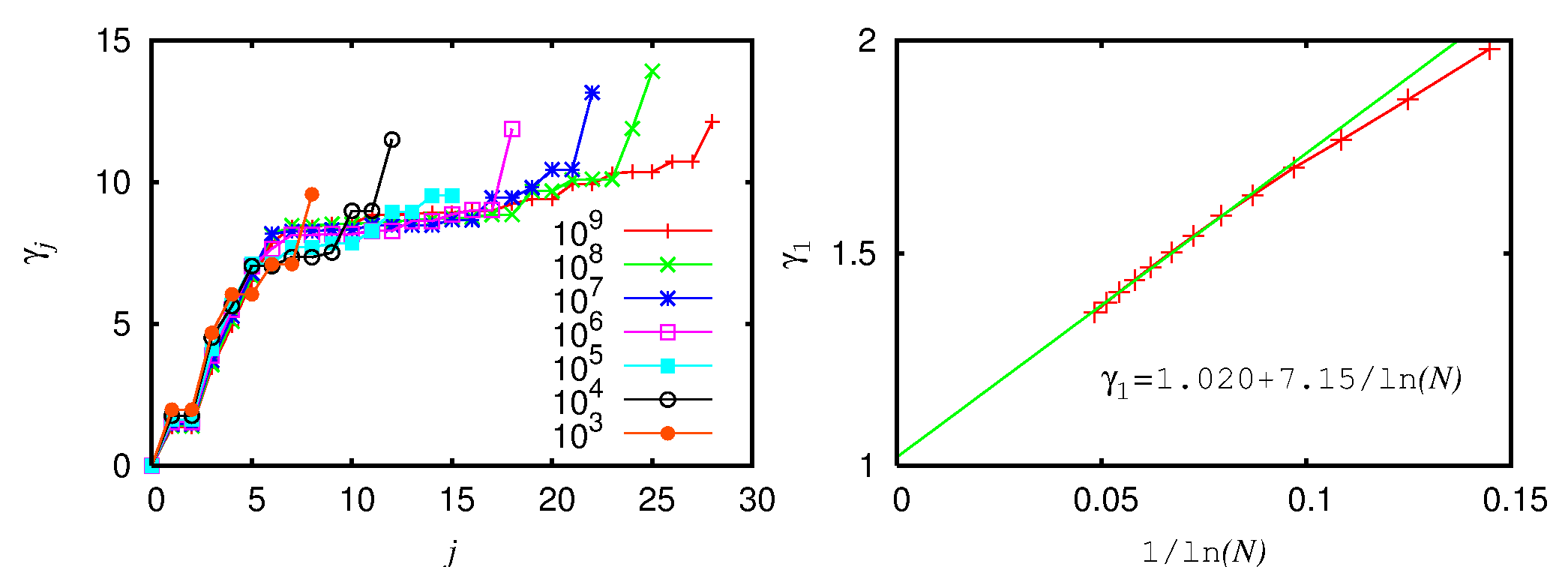
To study the evolution of the eigenvalue spectrum with $N$ it is actually convenient to introduce the variable $\gamma_{j}=-2\ln|\lambda_{j}|$. The dependence on $\gamma_{j}$ on the index $j$ is shown in left panel of Fig. 9. It appears that the $\gamma$-spectra for different values of $N$ fall roughly on the same curve except for the last one or two values of each spectrum. This universal curve can be roughly approximated by a piecewise linear function with two slopes $\approx 4/3$ for $0\leq j\leq 6$ and $\approx 1/7$ for $6\leq j\leq 28$.

We note that the convergence of the first nonzero $\gamma_{1}$ is compatible with the law $\gamma_{1}(N)\approx\gamma_{1}(\infty)+\Delta\gamma/\ln N$ with $\gamma_{1}(\infty)=1.020\pm 0.006$ and $\Delta\gamma=7.14\pm 0.09$ obtained from a fit in the range $10^{5}\leq N\leq 10^{9}$. This fit is actually very accurate as can be seen from the small error of $\gamma_{1}(\infty)$ and the right panel of Fig. 9. Once more, such a dependence indicates a very slow logarithmic convergence with the system size $N$.

• 

Figure 9: Left panel: dependence of $\gamma_{j}=2\ln|\lambda_{j}|$ on the index $j$ for the $l$ non-vanishing eigenvalues of $S$ and various matrix sizes $N$. Right panel: dependence of $\gamma_{1}$ on $(\ln N)^{-1}$ (red line with crosses). The green line corresponds to the fit $\gamma_{1}(N)=\gamma_{1}(\infty)+\Delta\gamma/\ln N$ for the range $10^{5}\leq N\leq 10^{9}$ (i.e. $(\ln N)^{-1}<0.09$) with $\gamma_{1}(\infty)=1.020\pm 0.006$ and $\Delta\gamma=7.14\pm 0.09$.

• 

Figure 10: Dependence of the PageRank vector $P$ (red curve) and the eigenvector $|\psi_{1}|$ (blue crosses) on PageRank index K for $N=10^{7}$. Here the eigenvalue is $\lambda_{1}=-0.28422+i\,0.38726$ ($|\lambda_{1}|=0.48037$, $\gamma_{1}=1.4663$; and the corresponding $\psi_{1}$ is normalized by the condition $\sum_{n}|\psi_{1}(n)|=1$); green curve shows the difference $|\Delta P|$ between the numerically computed PageRank $P$ (red curve) and semi-analytical computation of PageRank; for clarity $|\Delta P|$ is multiplied by a factor $10^{8}$.

In Fig. 10. we show the amplitude $|\psi_{1}|$ of the second eigenvector $\psi_{1}$ at $\lambda_{1}=-0.28422+i\,0.38726$ for $N=10^{7}$ versus the $K$ index. Despite some fluctuations this eigenvector seems to be close to the PageRank as far as the overall distribution of very large and small values is concerned. This behavior does not come as a surprise in view of the expansion [see Eq. (5)] :

$$\psi_{1}\propto\sum_{j=0}^{l-1}\lambda_{1}^{-j-1}\,v^{(j)}\quad.$$ (12)

In principle the fact that $|\lambda_{1}|$ is well below 1 indicates that the contributions of $v^{(j)}$ for larger values of $j$ increase. However, as we will discuss in the next section, the overall size of $v^{(j)}$ decays with increasing $j$ much faster than the increase by the factor $\lambda_{1}^{-j-1}$ and therefore mainly the first few terms of this sum contribute to $\psi_{1}$ in a similar way as for the PageRank (see Section 5).

Finally in Fig. 10, also the numerical difference of the PageRank determined by the standard power method and the semi-analytical expression (8) is shown. The relative difference is $\sim 10^{-10}$ for the full range of $K$ thus numerically confirming the accuracy of Eq. (8).

4.3 Numerical problems due to Jordan blocks

The question arises why the Arnoldi Method for both initial vectors, random and uniform, (and also direct numerical diagonalization for small matrix sizes $N\leq 10^{4}$) fail to confirm the analytical result that there are only $l=[\log_{2}(N)]$ non-zero eigenvalues $\lambda\neq 0$ of $S$. The reason is that the big subspace of dimension $N-l$ associated to the eigenvalue $\lambda=0$ with a lot of large Jordan blocks is numerically very problematic. This effect for such a defective eigenvalue is well known in the theory of numerical diagonalization methods [12]. To understand this a bit clearer consider a “perturbed” Jordan block of size $D$:

$$\left(\begin{array}[]{ccccc}0&1&\cdots&0&0\\ 0&0&\cdots&0&0\\ \vdots&\vdots&\ddots&\vdots&\vdots\\ 0&0&\cdots&0&1\\ \varepsilon&0&\cdots&0&0\\ \end{array}\right)$$ (13)

which has a characteristic polynomial $\lambda^{D}-(-1)^{D}\varepsilon$ and therefore complex eigenvalues that scale as $|\lambda|\sim\varepsilon^{1/D}$ as a function of the perturbation $\varepsilon$ while for $\varepsilon=0$ we have $\lambda=0$ with multiplicity $D$. Therefore a value of $\varepsilon\sim 10^{-15}$ due to numerical rounding errors may still produce strong numerical errors in the eigenvalues if $D$ is sufficiently large. In our case Fig. 8 shows that the eigenvalues obtained by the Arnoldi method are accurate for $|\lambda|\geq 10^{-2}$.

As can be seen in Fig. 8 there is also a difference in quality between the two initial vectors chosen for the Arnoldi Method. Using a random initial vector the Arnoldi method produces some wrong isolated eigenvalues in the intermediate regime $0.01\leq|\lambda|\leq 0.02$ and in the case $N=10^{7}$ some of the semi-analytical eigenvalues in the same regime are not accurately found. However, for the uniform initial vector the Arnoldi method produces rather accurate eigenvalues even for $|\lambda|\approx 0.005$. The reason is that the uniform initial vector corresponds (up to normalization) to the vector $v=e/N$. In view of Eq. (10) the Arnoldi method generates, at least in theory, exactly the $l$-dimensional subspace spanned by the vectors $v^{(j)}$ and should exactly break off at $n_{A}=l$ with a vanishing coupling matrix element from the subspace to the remaining space. However, due to numerical rounding errors and the fact that the vectors $v^{(j)}$ are badly conditioned, i.e. mathematically there are linearly independent but numerically nearly linearly dependent, the coupling matrix element is of order $10^{-3}$ (for $N=10^{7}$). As a consequence the Arnoldi method continues to generate new vectors producing a cloud of “artificial” eigenvalues inside a circle or radius $\sim 0.005$. These eigenvalues are generated by the above explained mechanism of perturbed Jordan blocks.

The Arnoldi method with a random initial vector produces a similar, slightly larger cloud, of such artificial eigenvalues but here, even without any numerical rounding errors, the method should not break off due to a bad choice of the initial vector and actually it even produces some “bad” eigenvalues outside the Jordan block generated cloud.

We mention that it is possible to improve the numerical behavior of the Arnoldi method with uniform initial vector by the following “tricks”: first we chose a different matrix representation of $S$ where the first basis vector (associated to the number “1”) is replaced by the uniform vector $e$ and second where the scalar product used for the Gram-Schmidt orthogonalization is modified with stronger weights $\sim n^{2}$ for the larger components. This modified Arnoldi method produces a very small coupling matrix element $\sim 10^{-10}$ (for $N=10^{7}$) at $n_{A}=l$ and numerically very accurate eigenvalues (up to $10^{-10}$) for all $l$ non-vanishing eigenvalues. If we force to continue the Arnoldi iterations ($n_{A}\gg l$) we obtain again a Jordan block generated cloud of eigenvalues but whose size is considerably reduced as compared to both original variants of the method.

5 Self-consistent determination of PageRank and analytic approximation

The eigenvalue equation of the PageRank: $P=C\,v+S_{0}\,P$ with $C=d^{\,T}\,P$ [see Eq. (2)] can be interpreted as a self-consistent equation for $P$ defining a very effective iterative method to determine $P$ in a few number of iterations. Let us define the following iteration procedure :

$$P^{(0)}=0\quad,\quad P^{(j+1)}=C\,v+S_{0}\,P^{(j)}\quad,\quad j=0,\,1,\,2,\,\ldots\ .$$ (14)

In principle the constant $C=d^{\,T}\,P$ is only obtained once the exact PageRank is known. Therefore in a practical application of this iteration, one first chooses some arbitrary non-vanishing value for $C$ and normalizes the PageRank once the procedure has converged. However, for reasons of notations we chose to keep the value $C=d^{\,T}\,P$ in Eq. (14) from the very beginning.

We note that the iteration (14) can formally be solved by the sum :

$$P^{(j)}=C\,\sum_{i=0}^{j-1}S_{0}^{i}\,v=C\,\sum_{i=0}^{j-1}v^{(i)}\ .$$ (15)

Since $S_{0}^{l}=0$ for $l=[\log_{2}(N)]$ the iteration not only converges but it actually provides the exact PageRank $P=P^{(l)}$ after a finite number of iterations when $j=l$ and in which case Eq. (15) coincides with our previous result (8).

We mention that the power method, where one successively multiplies the matrix $S=v\,d^{\,T}+S_{0}$ to an initial (normalized) vector is somewhat similar to (14) but with a very crucial difference. In the power method the constant $C$ is updated at each iteration according to $C^{(j)}=d^{\,T}\,P^{(j)}$ and here the initial vector must be different from $0$. We remind that the power method converges exponentially with an error $\sim|\lambda_{1}|^{j}$ where $\lambda_{1}$ being the second eigenvalue of $S$ with $|\lambda_{1}|\approx 0.5$ for $N=10^{9}$ and an extrapolated value $|\lambda_{1}|\approx 0.6$ in the limit $N\to\infty$. As can be seen in Fig. 11, the iteration (14) actually converges much faster than $|\lambda_{1}|^{j}$ which is simply due to fixing the constant $C$ from the beginning and not updating it with the iterations.

• 

Figure 11: Decay of the quantity $\delta_{j}=\|P^{(j)}-P\|_{1}$ representing the error of the approximate PageRank $P^{(j)}$ after $j$ iterations of Eq. (14) (for $N=10^{7}$). The left panel shows $\delta_{j}$ versus $j$ and the green line is obtained from the fit: $\ln(\delta_{j})=a_{3}-b_{3}\,j-c_{3}\,j^{2}$ with $a_{3}=1.6\pm 0.4$, $b_{3}=1.48\pm 0.08$ and $b_{3}=0.117\pm 0.004$. The right panel shows $-\ln(\delta_{j})$ versus $j$ and the green line is obtained from the fit: $\ln[-\ln(\delta_{j})]=a_{4}+b_{4}\,j$ for $j>12$ with $a_{4}=2.46\pm 0.03$ and $b_{4}=0.092\pm 0.002$. Note that both panels use a logarithmic representation for the vertical axis.

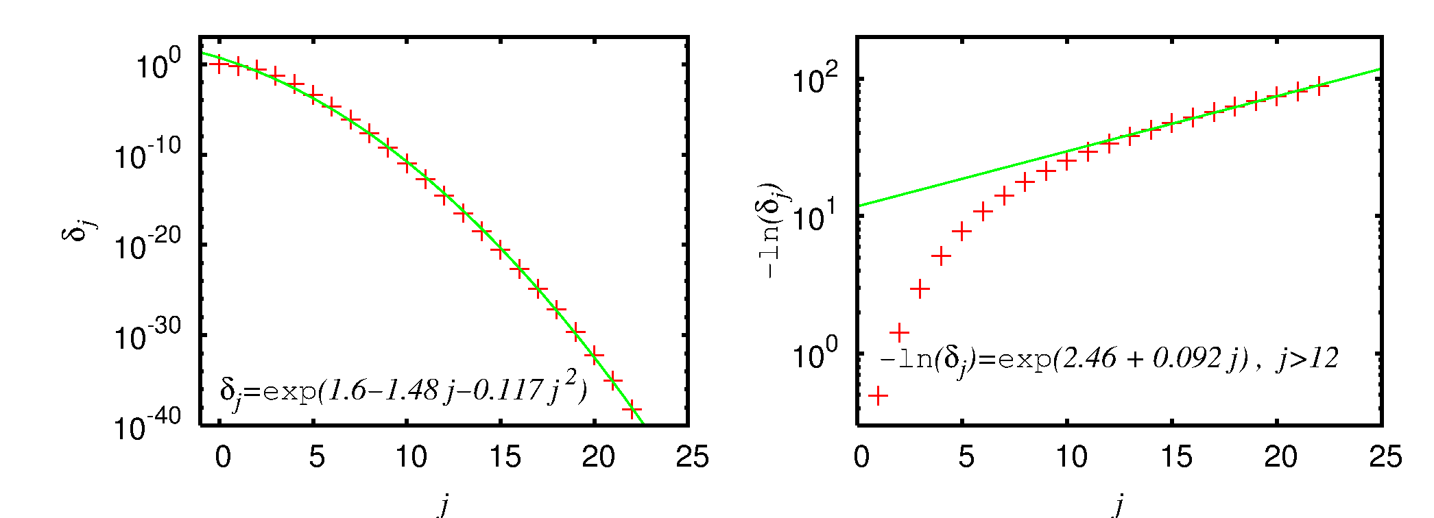
The norm $\delta_{j}=\|P^{(j)}-P\|_{1}$ of the error vector after $j$ iterations decays much faster than exponentially with $j$ as it is shown in Fig. 11. For $N=10^{7}$ one can quite well approximate the error norm by the fit : $\delta_{j}\approx\exp(1.6-1.48\,j-0.117\,j^{2})$ representing a quadratic function in the exponential. Furthermore, for $j$ close to $l$ we have the approximate ratio $\delta_{j}/\delta_{j-1}\approx 10^{-2}$ and not $0.5$-$0.6$ as the power method would imply. For $j>12$ one can actually identify a regime of superconvergence where the logarithm of the error behaves exponentially : $-\ln(\delta_{j})\approx\exp(2.46+0.092\,j)$ but the parameter range for $j$ is too small to decide if there is really superconvergence. However, both fits clearly indicate that the convergence is considerably faster than exponential.

• 

Figure 12: Left panel: Comparison of the first three PageRank approximations $P^{(j)}$ for $j=1,\,2,\,3$ obtained from Eq. (14) and the exact PageRank $P$ versus the PageRank index $K$. Right panel: Comparison of the dependence of the rescaled probabilities $nP$ and $nP^{(3)}$ on $n$. Both panels correspond to the case $N=10^{7}$.

As a consequence of the very rapid convergence dependent on the required precision, it is sufficient to apply the iteration (14) only a few number of times $j\ll l$ to obtain a reasonable approximation. For example, Fig. 12 shows for $N=10^{7}$ that on a logarithmic scale $P^{(3)}$ and $P$ are already very close.

This allows to obtain a very simple analytical approximation of the PageRank : $P\approx P^{(3)}=v^{(0)}+v^{(1)}+v^{(2)}$. For this let us rewrite the recursion $v^{(j+1)}=S_{0}\,v^{(j)}$ in a different way :

$$v^{(j+1)}_{n}=\sum_{m=2}^{[N/n]}\,\frac{M(mn,m)}{Q(mn)}\,v^{(j)}_{mn}\quad{\rm if}\quad n\geq 2\quad{\rm and}\quad v^{(j+1)}_{1}=0\quad,$$ (16)

where for given two integers $n$ and $m>1$ the multiplicity $M(n,m)$ is the largest integer such that $m^{M(n,m)}$ is a divisor of $n$ and $Q(n)=\sum_{m=2}^{n-1}M(n,m)$ is the number of divisors of $n$ (different from $1$ and $n$ itself) counting divisors several times according to their multiplicity. The appearance of the multiplicity $M(mn,n)$ in (16) is not very convenient for numerical evaluations. Either one recalculates the multicity at each use or one sacrifices a big amount of memory to store them. It is actually possible to rewrite Eq. (16) in a way that the multiplicities no longer appear explicitely. For this we note that the case $M(mn,n)\geq 2$ implies only to those values of $m$ such that $n$ is a divisor of $m$ implying $m=\tilde{m}n$ and $mn=\tilde{m}n^{2}$. This produces a second sum where one uses the multiples of $n^{2}$ and in a similar way a further sum with multiples of $n^{3}$ for the cases $M(mn,n)\geq 3$ and so on. For $n\geq 2$, we may therefore rewrite Eq. (16) in the following equivalent expression :

$$v^{(j+1)}_{n}=\sum_{m=2}^{[N/n]}\,\frac{1}{Q(mn)}\,v^{(j)}_{mn}+\sum_{\nu\geq 2}^{n^{\nu}\leq N}\sum_{m=1}^{\ [N/n^{\nu}]}\,\frac{1}{Q(mn^{\nu})}\,v^{(j)}_{mn^{\nu}}$$ (17)

where each term in the sum of $\nu$ takes into account for the contributions with $M(mn,m)=\nu$. Note that the extra sums start at $m=1$ since $n\geq 2$ and therefore $mn^{\nu}>n$ even for $m=1$. The above PageRank iteration (14) can be written in a similar way (see below) but for practical purposes, numerical or analytical, it is actually more convenient to use the recurrence for the vectors $v^{(j)}$ and to add them to obtain the PageRank according to Eq. (15).

Both Eqs. (16) and (17) are also very efficient for a numerical evaluation, especially in terms of memory usage, since the matrix $S_{0}$ is represented by “only” $N$ integer values $Q(n)$, $n=1,\,\ldots,\,N$ which is much less than the number ($\sim N\ln N$) of non-zero double-precision matrix elements of $S_{0}$ (even completely taking into account the sparse structure of $S_{0}$). When using Eq. (16) one can recalculate at each time the multiplicities $M(n,m)$ which is not very expensive. However, it turns out that the additional sums in Eq. (17) are slightly more effective than this recalculation. Furthermore, for the iteration of $v^{(j)}$ the number of non-vanishing elements is reduced by a factor of two at each iteration. As a consequence we may replace in Eqs. (16) and (17) $N$ by $[N\,2^{-j}]$ and thus considerably reduce the computation time. We note that the direct iteration of $P^{(j)}$ instead $v^{(j)}$ does not have this advantage. Actually, in terms of numerical computation time the approximation to stop after few iterations is not very important since in any case the higher order corrections require less computation time. Using the iteration (17), we have been able to determine numerically the vectors $v^{(j)}$ and therefore the PageRank, the coefficients $c_{j}$ and the resulting $l=[\log_{2}N]$ non-zero eigenvalues of $S$ for system sizes up to $N=10^{9}$.

In addition, Eq. (16) allows also for some analytical approximate evaluation of the first vectors. The initial vector is $v^{(0)}_{n}=1/N$. Let us try to evaluate the next two vectors $v^{(1)}_{n}$ and $v^{(2)}_{n}$ for the most important case where $n$ is a prime number $p$. Furthermore, in the sum (16) the most important contributions arise for $m$ also being a prime number $q$ such that $Q(qp)=2$ and $M(qp,p)=1$ (except for the case $q=p$ which we neglect) resulting in :

$$v^{(1)}_{p}\approx\sum_{q=2,{\rm\ prime}}^{[N/p]}\frac{1}{2N}=\frac{1}{2N}\,\pi\left(\left[\frac{N}{p}\right]\right)\approx\frac{1}{2p(\ln N-\ln p)}$$ (18)

where $\pi(n)\approx n/\ln(n)$ (for $n\gg 1$) is the number of prime numbers below $n$. However, these values of $v^{(1)}_{n}$ at prime numbers $n=p$ do not contribute in (16) for the next iteration $j=1$ when trying to determine $v^{(2)}$. To obtain the leading contributions in $v^{(2)}$ we need $v^{(1)}_{n}$ for $n=p_{1}\,p_{2}$ being a product of two prime numbers. In this case, we have $Q(q\,p_{1}\,p_{2})=2^{3}-2=6$ if $q,\,p_{1},\,p_{2}$ are three different prime numbers. Assuming $p_{1}\neq p_{2}$ and neglecting the complications from the few cases $q=p_{1}$ or $q=p_{2}$, we find that :

$$v^{(1)}_{p_{1}\,p_{2}}\approx\frac{1}{6N}\,\pi\left(\left[\frac{N}{p_{1}\,p_{2}}\right]\right)\approx\frac{1}{6p_{1}\,p_{2}\,(\ln N-\ln p_{1}-\ln p_{2})}\ .$$ (19)

For the case $n=p^{2}$, i.e. $p_{1}=p_{2}=p$, we have $Q(qp^{2})=5$ (since $p$ has multiplicity 2) resulting in :

$$v^{(1)}_{p^{2}}\approx\frac{1}{5N}\,\pi\left(\left[\frac{N}{p^{2}}\right]\right)\approx\frac{1}{5p^{2}\,(\ln N-2\,\ln p)}\ .$$ (20)

From (16) for $j=1$ and (19) we obtain :

$$v^{(2)}_{p}\approx\frac{1}{12N}\sum_{q=2,{\rm\ prime}}^{[N/(2p)]}\pi\left(\left[\frac{N}{p\,q}\right]\right)\ .$$ (21)

Here we have reduced the sum from $q\leq[N/p]$ to $q\leq[N/(2p)]$ since $\pi\left([N/(pq)]\right)$ is non zero only for $N/(pq)\geq 2$ and therefore $q\leq N/(2p)$. Now, we replace the sum $\sum_{q}(\cdots)$ over the prime numbers by an integral $\int dq\,\pi^{\prime}(q)\,(\cdots)$ where $\pi^{\prime}(q)\approx 1/\ln(q)$ is the average density of prime numbers at $q$ resulting in :

$$v^{(2)}_{p} \approx \frac{1}{12N}\int_{2}^{N/(2p)}dq\,\pi\left(\left[\frac{N}{p\,q}\right]\right)\,\pi^{\prime}(q)$$

$$\approx \frac{1}{12p}\int_{2}^{N/(2p)}\frac{dq}{q}\,\frac{1}{\Bigl{(}\ln(N/p)-\ln q\Bigr{)}\ln q}$$

$$= \frac{1}{12p}\int_{\ln 2}^{\ln\left(N/(2p)\right)}du\,\frac{1}{\Bigl{(}\ln(N/p)-u\Bigr{)}\,u}$$

$$= \frac{1}{6p\,\ln(N/p)}\left(\ln\ln\left(\frac{N}{2p}\right)-\ln\ln 2\right)\ .$$ (22)

From (18) and (22) we obtain the PageRank approximation at integer values

$$P_{p}\approx P^{(3)}_{p}\approx C(\frac{1}{N}+v^{(1)}_{p}+v^{(2)}_{p})\approx\frac{C}{2p\ln N}\left(1-\ln\ln 2+\frac{\ln\ln N}{3}\right)$$ (23)

where we have assumed that $N\gg p$ and replaced $\ln(N/p)=\ln N-\ln p\approx\ln N$ and $C$ is the same constant as used in (14).

The important point with this expression is that it is of the form $P_{p}\approx C_{N}/p$ where $C_{N}$ is a constant depending on $N$. In order to compare with our above results, especially in Fig. 2, we have to replace $p$ by the $K$ index. Assuming that the $K$ index is dominated by the prime numbers we have $K=\pi(p)\approx p/\ln p$ implying $p\approx K\ln p\approx K\,\ln K$ thus providing the behavior $P(K)\approx C_{N}/(K\,\ln K)$ already conjectured above based on the numerical results. Concerning the numerical value of the constant $C_{N}$ we find that, at $N=10^{7}$, it is roughly one order of magnitude too small as compared to the numerical results.

We remind that the considerations leading to the expression (23) are based on a lot of assumptions and quite crude approximations, especially the replacement of $\pi(n)\approx n/\ln(n)$, even if $n={\cal O}(1)$, and we have neglected a lot of contributions from numbers with more factors in their prime factor decomposition which are most likely responsible for the reduced numerical prefactor. Furthermore, the assumption that the PageRank is dominated by prime numbers is not completely exact since certain non-prime numbers with a small number of factors intermix with larger prime numbers in the PageRank, thus modifying the dependence of the prime numbers on the $K$ index from $p\approx K\,\ln(K)$ to $p\approx K\,(1.36+0.323\ln K)$ according to the fit in Fig. 6 for $N=10^{7}$. However, despite the approximations, we recover the leading parametric dependence of $P\sim 1/(K\,\ln K)$.

• 

Figure 13: Left panel: The full lines correspond to the dependence of PageRank probability $P(K)$ on PageRank index $K$ for the matrix sizes $N=10^{7}$, $10^{8}$, $10^{9}$ with the PageRank evaluated from the expression (8) using the efficient numerical method based on Eq. (17). The green crosses correspond to the PageRank obtained by the power method (PM) for $N=10^{7}$; the dashed straight line shows the Zipf law dependence $P\sim 1/K$. Right panel: same as in left panel (without data from the power method) for a simplified model for the Google matrix of integers where all multiplicities $M(n,m)$ are replaced by 1, i.e. $n$ is to linked to its divisors $m$ only once even if $n$ can be divided several times by $m$. The PageRank was numerically evaluated by the same efficient method using Eqs. (8) and (16) with $M(n,m)=1$.

• 

Figure 14: Dependence of $|\Delta K|=|K_{n}(N_{2})-K_{n}(N_{1})|$ on integer $n$ for matrix sizes $N_{1}=10^{8},N_{2}=10^{9}$ (green points) and $N_{1}=10^{7},N_{2}=10^{8}$ (red points). Left and right panels show the same data in normal and log-log scales. Note the strongly reduced vertical scale of the left panel as compared to the left panel of Fig. 7. The vertical scale of the right panel was not reduced allowing a direct comparison with the right panel of Fig. 7. The data was obtained by the same efficient numerical method as in the left panel of Fig. 13.

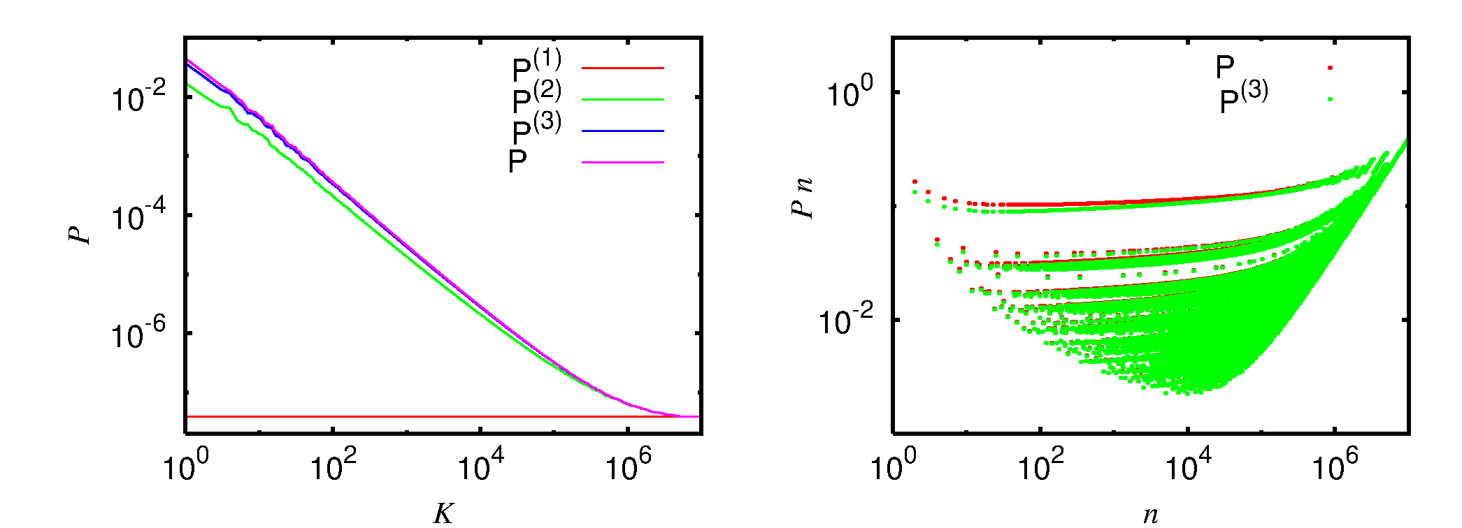
The PageRank dependence $P(K)$ obtained from the expression (8) using the efficient numerical method based on Eq. (17) is shown in Fig. 13 (left panel) for $N=10^{7},10^{8},10^{9}$. For $N=10^{7}$ these data agree with the computation result by the Arnoldi power method with the numerical accuracy of the order of $10^{-10}$ (see also Fig. 10). This confirms the efficiency of our semi-analytical computation of the PageRank.

We note that it may be useful to consider a simplified model for the Google matrix of integers when multiplicity of all divisors is taken to be unity. The numerical fit of data shows that in this case the number of links scales as $N_{\ell}=N\,(a_{\ell}+b_{\ell}\ln N)$ with $a_{\ell}=-1.838\pm 0.002$, $b_{\ell}=0.999\pm 0.0002$. For this model we have the same expression (16) but with the replacements $M(nm,m)\to 1$ and $Q(n)\to Q^{*}(n)$ where $Q^{*}(n)$ is the number of divisors of the integer $n$ excluding 1 and $n$ itself without multiplicities, e. g. $Q^{*}(2)=0,\,Q^{*}(3)=0,\,Q^{*}(4)=1,\,\ldots$. Note that this quantity is given by the expression $Q^{*}(n)=\left(\prod_{j}(\mu_{j}+1)\right)-2$ where $\mu_{j}$ are the exponents in the prime factor decomposition of $n=\prod_{j}p_{j}^{\mu_{j}}$.

The dependence of the PageRank on $K$ for the simplified model is shown in the right panel of Fig. 13. It shows practically the same behavior as in the main model shown in the left panel. In this case the analytical expression for the PageRank $P$, obtained from the first three terms, has a very simple form

$$P_{n}\approx P^{(3)}_{n}=\sigma_{N}\Biggl{(} 1 +\sum_{m_{1}=1}^{[N/n]}\frac{1}{Q^{*}(m_{1}n)}$$

$$+\sum_{m_{1}=2}^{[N/n]}\sum_{m_{2}=2}^{\ [N/(nm_{1})]}\frac{1}{Q^{*}(m_{1}n)}\frac{1}{Q^{*}(m_{2}m_{1}n)}\Biggr{)}$$

where $N$ is the matrix size and $\sigma_{N}$ is the global normalization constant determined by the condition $\sum_{n=1}^{n=N}P_{n}=1$. This simple formula gives a good description of the PageRank behavior shown in the right panel of Fig. 13. Indeed, the direct count shows that the ratio $R_{ms}$ of the total number of links $N_{\ell}$ for both models (counted with or without multiplicities) approaches to unity for large matrix sizes. For example, we have $R_{ms}=1.184$ ($N=1000$), $1.102$ ($10^{5}$), $1.070$ ($10^{7}$), $1.052$ ($10^{9}$). Thus we think that in the limit of large $N$ both models converge to the same type of behavior. It is possible that the simplified model may be more suitable for further analytical analysis. However, in this work we present data for the simplified model only in the right panel of Fig. 13.

Using the PageRank data obtained by the self-consistent approach for large $N=10^{7},10^{8},10^{9}$ we can analyze the convergence of the PageRank order $K_{n}$ at larger sizes compared to those used in Fig. 7. These new results for variation of $|\Delta K|$ are presented in Fig. 14. They show that the variation $|\Delta K|$ decreases with the increase of $N$ from $10^{7}$ up to $10^{9}$ even if the process is slow. A direct comparison shows that the first deviation in the order $K_{n}$ appears at $K=K_{s}=13$ (comparing $N=10^{6}$ vs. $10^{7}$), $K_{s}=27$ ($10^{7}$ vs. $10^{8}$), $K_{s}=30$ ($10^{8}$ vs. $10^{9}$). We find that the stable range interval $K_{s}$ grows with $N$ but this growth seems logarithmic like with $K_{s}\sim\ln N$. Such a growth seems to be natural in the view of logarithmic convergence of the second eigenvalue $\lambda_{1}$ discussed above and all logarithmic factors appearing in the density of primes. We also note that the value of $K_{s}$ is significantly smaller than the value of $K_{d}$ at which the first degenerate flat plateau appears in the PageRank $P(K)$ and hence these degeneracies do not affect the order of the first $K_{s}$ integers.

On the basis of the obtained results we conclude that for our maximal matrix size $N=10^{9}$ we have convergence of the first 32 values of $K_{n}$. These numbers $n$, corresponding to the values of $K=1,\,2,\,\ldots,\,32$, are $n=2$, $3$, $5$, $7$, $4$, $11$, $13$, $17$, $6$, $19$, $9$, $23$, $29$, $8$, $31$, $10$, $37$, $41$, $43$, $14$, $47$, $15$, $53$, $59$, $61$, $25$, $67$, $12$, $71$, $73$, $22$, $21$. There are about 30% of non-primes among these values. We mention that the positions of the first non-primes $4,\,6,\,9$ can be already obtained from the first order approximations of $v^{(1)}$ discussed above. According to (18) the relative weight of a prime number in first order is $1/(2p)$. For the two square numbers $4$ and $9$ the weight is according to (20) either $1/(5\times 4)=1/(2\times 10)$ or $1/(5\times 9)=1/(2\times 22.5)$ explaining that $4$ is between the primes $7$ and $11$ and that $9$ is between $19$ and $23$. For the product $6=2\times 3$ we have according to (19) the weight $1/(6\times 6)=1/(2\times 18)$ implying that $6$ is between 17 and 19. However, this simple argument does not work for other numbers, for example for $10$ (or $14$) it would imply an incorrect position between $29$ and $31$ ($41$ and $43$). We mention that more numerical data are available at the web page [15].

For the simplified model we find at $N=10^{9}$ for the first values $K=1,\,2,\,\ldots,\,32$ a slightly different order of integers $n=2$, $3$, $5$, $4$, $7$, $11$, $13$, $17$, $9$, $6$, $19$, $8$, $23$, $29$, $31$, $10$, $37$, $41$, $43$, $14$, $47$, $15$, $53$, $25$, $59$, $16$, $61$, $12$, $67$, $71$, $22$, $21$. Here the absence of multiplicities increases the weight for square numbers of primes to $1/(4p^{2})$ implying that these numbers are slightly advanced in the $K$ order as compared to our main model. The modified weight for $9$ is $1/(2\times 18)$ coherent with new position between $17$ and $19$ (with $6$ having the same first order weight as $9$ and also being between $17$ and $19$). For $4$ the weight is increased from $1/(2\times 10)$ to $1/(2\times 8)$. However, this increase is not sufficient to explain the new position of $4$ between $5$ and $7$.

One might mention as a curiosity a special “prime integer network model” where a non-prime number $n$ is only linked to its prime factors (and not to all of its divisors). In this case the matrix $S_{0}$ is strongly simplified such that $S_{0}^{2}=0$, i.e. $l=2$ being independent of the system size and hence there are only two non-vanishing eigenvalues of the Google matrix which are $\lambda_{0}=1$ and $\lambda_{1}=c_{0}-1\approx-1+1/\ln N$ where $c_{0}=(\pi(N)+1)/N\approx 1/\ln N$ is the ratio of the number of primes and unity to $N$. This is simply seen from the definition of $c_{j}$ in Eq. (6) and the trace $c_{0}=\lambda_{0}+\lambda_{1}$ of the matrix (11) which is of size $2\times 2$ for this case. According to (5) the PageRank $P$ and the second eigenvector $\psi_{1}$ are given by $P\propto e+v^{(1)}$ and $\psi_{1}\propto e-v^{(1)}/(1-1/\ln N)$ where $e$ is the vector with all components equal to unity and $v^{(1)}$ is a vector such that $v_{n}^{(1)}=0$ for non-prime numbers $n$ or $n=1$ and $v_{n}^{(1)}$ for prime numbers $n=p$ is given by an equation similar to Eq. (16) for $j=0$ with $v_{nm}^{(0)}$ being replaced by unity and multiplicities and number of divisors adapted for the prime integer network model. Here both versions, with or without multiplicities are possible. The eigenvalues do not depend on the version but the eigenvectors do. For both cases it is pretty obvious that the $K$ index gives exactly the sequence of prime numbers below $N$ in increasing order followed by a large degenerated plateau for the non-prime integer numbers. Note that here the second eigenvalue converges to $-1$ with a correction $1/\ln(N)$ for large $N$ thus closing the gap in $|\lambda|$ of the Google matrix.

6 Discussion

In this work we constructed the Google matrix of integers based on links between a given integer $n$ and its divisors. The numerical analysis based on the Arnoldi method allowed us to show that the PageRank $P(K_{n})$ of this directed network decays with PageRank index $K_{n}$ of an integer $n$ approximately as $P(K_{n})\sim 1/(K_{n}\ln K_{n})$ being similar to those of the Zipf law and those found for the WWW. However, the spectrum of the Google matrix has a large gap appearing between the unit eigenvalue and other eigenvalues while the spectrum of the Google matrix of WWW usually has no gap. We developed an efficient semi-analytical method to compute the PageRank of integers which allowed us to determine the dependence $P(K_{n})$ up to matrix size of one billion. We show that the dependence of PageRank on the integer number $n$ is characterized by a series of branches corresponding to primes, semi-primes and numbers with a higher products of primes. Our data show a logarithmic like convergence of PageRank order of integers to a fixed order in the limit of matrix size going to infinity.

References

- [1] Hardy G H and Wright E M 2008, An introduction to the theory of numbers, (6th ed., Oxford: Oxford University Press)
- [2] Crandall R and Pomerance C 2005, Prime numbers: a computational perspective, (Berlin: Springer-Verlag)
- [3] Berry M V 1991 Some quantum-to-classical asymptotics, in Les Houches Lecture Series LII (1989), Eds. M-J Giannoni, A Voros and J Zinn-Justin, North-Holland, Amsterdam, 251
- [4] Berry M V and Keating J P 1999 SIAM Review 41 236
- [5] Srednicki M 2011 Phys. Rev. Lett. 107 100201
- [6] Markov A A 1906 Rasprostranenie zakona bol’shih chisel na velichiny, zavisyaschie drug ot druga, Izvestiya Fiziko-matematicheskogo obschestva pri Kazanskom universitete, 2-ya seriya, 15 135 (in Russian) [English trans.: Extension of the limit theorems of probability theory to a sum of variables connected in a chain reprinted in Appendix B of: Howard R A 2007 Dynamic Probabilistic Systems, volume 1: Markov models, Dover Publ. ]
- [7] Brin S, Page L 1998 Comput. Netw. ISDN Syst. 30 107
- [8] Langville A M and Meyer C D 2006 Google’s PageRank and Beyond: The Science of Search Engine Rankings, (Princeton: Princeton University Press)
- [9] Frahm K M, Georgeot B and Shepelyansky D L 2011 J. Phys, A: Math. Theor. 44 465101
- [10] Donato D, Laura L, Leonardi S and Millozzi S 2004 Eur. Phys. J. B 38 239
- [11] Pandurangan G, Raghavan P and Upfal E 2005 Internet Math. 3 1
- [12] Stewart G W 2001 Matrix Algorithms Volume II: Eigensystems, (SIAM)
- [13] Frahm K M and Shepelyansky D L 2010 Eur. Phys. J. B 76, 57
- [14] Zipf G K 1949 Human Behavior and the Principle of Least Effort, Addison-Wesley, Boston
-
[15]
Web page PageRank of integers
http://www.quantware.ups-tlse.fr/QWLIB/pagerankofintegers/