MOA 2010-BLG-477Lb: constraining the mass of a microlensing planet from microlensing parallax, orbital motion and detection of blended light

Abstract

Microlensing detections of cool planets are important for the construction of an unbiased sample to estimate the frequency of planets beyond the snow line, which is where giant planets are thought to form according to the core accretion theory of planet formation. In this paper, we report the discovery of a giant planet detected from the analysis of the light curve of a high-magnification microlensing event MOA 2010-BLG-477. The measured planet-star mass ratio is $q=(2.181\pm 0.004)\times 10^{-3}$ and the projected separation is $s=1.1228\pm 0.0006$ in units of the Einstein radius. The angular Einstein radius is unusually large $\theta_{\rm E}=1.38\pm 0.11$ mas. Combining this measurement with constraints on the “microlens parallax” and the lens flux, we can only limit the host mass to the range $0.13<M/M_{\odot}<1.0$. In this particular case, the strong degeneracy between microlensing parallax and planet orbital motion prevents us from measuring more accurate host and planet masses. However, we find that adding Bayesian priors from two effects (Galactic model and Keplerian orbit) each independently favors the upper end of this mass range, yielding star and planet masses of $M_{*}=0.67^{+0.33}_{-0.13}\ M_{\odot}$ and $m_{p}=1.5^{+0.8}_{-0.3}\ M_{\rm JUP}$ at a distance of $D=2.3\pm 0.6$ kpc, and with a semi-major axis of $a=2^{+3}_{-1}$ AU. Finally, we show that the lens mass can be determined from future high-resolution near-IR adaptive optics observations independently from two effects, photometric and astrometric.

1 Introduction

Gravitational microlensing is an important method to detect extrasolar planets (Mao & Paczyński, 1991; Bennett, 2008; Gaudi, 2010). The method is sensitive to planets not easily accessible to other methods, in particular cool and small planets at or beyond the snow line (Beaulieu et al., 2006; Bennett et al., 2008), and free-floating planets (Sumi et al., 2011). The snow line represents the location in the protoplanetary disk beyond which ices can exist (Lecar et al., 2006; Kennedy et al., 2007; Kennedy & Kenyon, 2008) and thus the surface density of solids is highest (Lissauer, 1987). According to the core accretion theory of planet formation (Lissauer, 1993), the snow line plays a crucial role because giant planets are thought to form in the region immediately beyond the snow line. Therefore, microlensing planets can provide important constraints on planet formation theories, in particular by measuring the mass function beyond the snow line (Gould et al., 2010; Sumi et al., 2010; Cassan et al., 2012).

A major component of current planetary microlensing experiments is being carried out in survey and follow-up mode, where survey experiments are conducted in order to maximize the event rate by monitoring a large area of the sky one or several times per night, while follow-up experiments are focused on events alerted by survey observations to densely cover planet-induced perturbations. In this mode, high-magnification events are important targets for follow-up observations. This is because the source trajectories of these events always pass close to the central perturbation region and thus the sensitivity to planets is extremely high (Griest & Safizadeh, 1998; Rhie et al., 2000; Rattenbury et al., 2002; Abe et al., 2004; Han, 2009). In addition, the time of the perturbation can be predicted in advance so that intensive follow-up observation can be prepared. This leads to an observational strategy of monitoring high-magnification events as intensively as possible, regardless of whether or not they show evidence of planets. As a result, the strategy allows one to construct an unbiased sample to derive the frequency of planets beyond snow line (Gould et al., 2010). For the alternative low-magnification channel of detection, see for instance Sumi et al. (2010).

In this paper, we report the discovery of a giant planet detected from the analysis of the light curve of a high-magnification microlensing event MOA 2010-BLG-477. Due to the high magnification of the event, the perturbation was very densely covered, enabling us to place constraints on the physical parameters from the higher-order effects in the lensing light curve induced by finite source effects as well as the orbital motion of both the lens and the Earth. We provide the most probable physical parameters of the planetary system, corresponding to a Jupiter-mass planet orbiting a K dwarf at about 2 AU, the system lying at about 2 kpc from Earth.

2 Observations

The event MOA 2010-BLG-477 at coordinates (RA, DEC)=($18^{\rm h}06^{\rm m}07.44^{\rm s},-31^{\circ}27\arcmin 16.12\arcsec)$ (J2000.0), $(l,b)=(0.046^{\circ},-5.095^{\circ})$ was detected and announced as a microlensing alert event by the Microlensing Observations in Astrophysics (MOA: Bond et al., 2001; Sumi et al., 2003) collaboration on 2010 August 2 ($\rm HJD^{\prime}=HJD-2450000=5410.9$) using the 1.8 m telescope of Mt. John Observatory in New Zealand. The event was also observed by the Optical Gravitational Lensing Experiment (OGLE: Udalski, 2003) using the 1.3m Warsaw telescope of Las Campanas Observatory in Chile.

Real-time modeling based on the rising part of the light curve indicated that the event would reach very high magnification and enabled us to predict the time of the peak. Followed by this second alert, the peak of the light curve was densely covered by follow-up groups of the Probing Lensing Anomalies NETwork (PLANET) (Beaulieu et al., 2006), Microlensing Follow-Up Network ($\mu$FUN) (Gould et al., 2006), RoboNet (Tsapras et al., 2009), and Microlensing Network for the Detection of Small Terrestrial Exoplanets (MiNDSTEp) (Dominik et al., 2010). More than twenty telescopes were used for the follow-up observations, including PLANET 1.0m of South African Astronomical Observatory (SAAO) in South Africa, PLANET 1.0m of Mt. Canopus Observatory in Tasmania, Australia, PLANET 0.6m Perth Observatory in Australia, PLANET 0.4m ASTEP telescope at Dome C, Antarctica, $\mu$FUN 1.3m SMARTS telescope of the Cerro Tololo Inter-American Observatory (CTIO), Chile, $\mu$FUN 0.4m of Auckland Observatory, $\mu$FUN 0.36m of Farm Cove Observatory (FCO), $\mu$FUN 0.36m of Kumeu Observatory, $\mu$FUN 0.4m of Possum Observatory, $\mu$FUN 0.4m of Vintage Lane Observatory (VLO), $\mu$FUN 0.3m of Molehill Astronomical Observatory (MAO), all in New Zealand, $\mu$FUN 0.46m of Wise Observatory, Israel, $\mu$FUN 0.8m of Teide Observatory at Canary Islands (IAC), Spain, $\mu$FUN 0.6m of Pico dos Dias Observatory, Brazil, RoboNet 2.0m of Faulkes North (FTN) in Hawaii, U.S.A., RoboNet 2.0m of Faulkes South (FTS), Australia, RoboNet 2.0m of Liverpool (LT) at Canary Islands, Spain, MiNDSTEp 1.54 m Danish telescope at La Silla, Chile, and MiNDSTEp 1.2m Monet North telescope at McDonald Observatory, U.S.A..

Please note that this paper reports the first microlensing observations from Antarctica. Unfortunately, the data quality of these pioneering observations was not high enough to be included into the models, but we give a short overview in Appendix A. In order to better constrain the second-order effects, new observations were taken at the $\mu$FUN 1.3 m SMARTS telescope at CTIO during the 2011 campaign.

To better characterize the lensed source star, spectroscopic observations were conducted near the peak of the event ($\rm HJD^{\prime}=5422.5$) by using the B&C spectrograph on the 2.5 m du Pont telescope at Las Campanas Observatory in Chile. The resolution was $R=1400$, corresponding to $\Delta\lambda=4.6$ Å. A comparison between the observed spectrum and synthetic ones was conducted to derive the effective temperature, gravity and metallicity of the source star. The usable part of the spectrum is only $\sim 1000$ Å  due to some scattered light issues with the instrument, particularly a problem for this faint star. We started by fitting standard stars using H$\alpha$, MgB, and NaD, but found that fits with H$\alpha$ alone resulted in the most accurate temperatures, so this is the diagnostic we used. The derived parameters of the source star are $T_{\rm eff}=5950\pm 150$ K for $\log g=4.0$ and a solar metallicity. The corresponding fit to the H$\alpha$ line is shown in Figure 1.

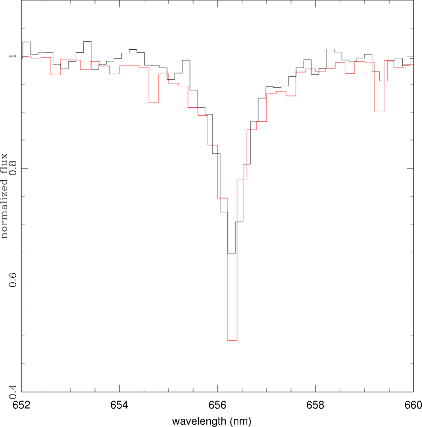
Figure 1: Reduced spectrum with an overplotted synthetic spectrum for the adopted source characteristics, namely $T_{\rm eff}=5950$ K, $\log g=4.0$ and solar metallicity.

The data collected by the individual groups were initially reduced using various photometry codes developed by the individual groups. For the data sets from SAAO, FTS, Possum, Canopus, Perth, Danish and Monet North, we use photometry from rereductions obtained with the pySIS package, described in more details in Appendix B.

Figure 2 shows the light curve of the event. The event is highly magnified with a peak magnification $A\sim 400$. Outside of the region ${\rm HJD^{\prime}}=[5417,5425]$, the light curve is consistent with a standard single-lens curve (Paczyński, 1986). The perturbation is composed of two spikes at ${\rm HJD^{\prime}}\sim 5420.4$ and 5420.9 and two bumps at ${\rm HJD^{\prime}}\sim 5421.0$ and 5422.4.

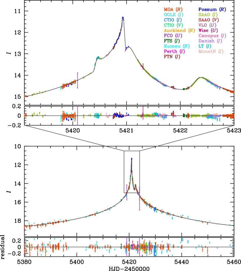
Figure 2: Light curve of the microlensing event MOA 2010-BLG-477. Data from different observatories are distinguished by different colors. The upper panel shows the enlargement of the region of perturbation near the peak of the light curve. Note that the model light curve corresponds to the best-fit solution of the model considering both parallax and orbital motion and the corresponding parameters are presented in Table 1.

3 Strategic Overview

As in the great majority of planetary microlensing events, we are able to measure the ”angular Einstein radius” (projected on the sky) $\theta_{\rm E}$, but not the projected Einstein radius (projected on the observer plane) $\tilde{r}_{\rm E}$. Consequently, it is challenging to estimate the physical parameters of the lens. The two radius quantities are related to those (Gould, 2000b, see) by

$$\theta_{\rm E}^{2}=\kappa\,\pi_{\rm rel}\,M;\quad\pi_{\rm E}^{2}=\frac{\pi_{\rm rel}}{\kappa\,M};\quad\tilde{r}_{\rm E}=\frac{{\rm AU}}{\pi_{\rm E}}$$ (1)

where $\kappa\equiv 4GM/{\rm AU}c^{2}\sim 8.1439\,{\rm mas}\,M_{\odot}^{-1}$, $M$ is the lens mass in $M_{\odot}$, and $\pi_{\rm rel}={\rm AU}(1/D_{L}-1/D_{S})$ is the lens-source relative parallax ($D_{L}$ and $D_{S}$ are the lens and source distances). Since $\theta_{\rm E}$ is well measured, the product $\pi_{\rm rel}\,M$ is also well determined, but in the present case, the ratio $\pi_{\rm rel}/M$ is poorly constrained, and so it is difficult to estimate $M$ alone. In this section, we provide an overview of the various techniques that we use to place constraints on the individual quantities $\pi_{\rm rel}$ and $M$.

We will show that here $\theta_{\rm E}$ is large enough to enable a substantial constraint from upper limits on the lens flux. That is, from Equation (1), large $\theta_{\rm E}$ implies large $M$ or $\pi_{\rm rel}$, both of which lead to brighter lenses. This will lead to the unambiguous conclusion that the lens is nearby, $D_{L}\lesssim 3\,$kpc, with mass $M\lesssim 1\,M_{\odot}$.

The light curve of this event enables stronger constraints than is usually the case because we are able to obtain a measurement of one of the microlens parallax component. The microlens parallax is actually a vector, $\mbox{\boldmath$\pi$}_{\rm E}$, with the magnitude given by Equation (1) and the direction by the lens-source relative motion (Gould et al., 1994). One component of the parallax only weakly constrains the scalar $\pi_{\rm E}$, but it constrains the direction of proper motion, which will be very important for future observations (see below). Moreover, one parallax component actually does provide a robust lower limit on the mass $M\gtrsim 0.13\,M_{\odot}$ and distance $D_{L}\gtrsim 0.5\,$kpc.

To proceed further, we must apply a Bayesian analysis, but here as elsewhere we are more fortunate than is typical. As always, there are Bayesian priors from a Galactic model, and in this case these strongly prefer the upper end of the mass/distance range permitted by the light curve.

But in addition, the reason that only one dimension of $\mbox{\boldmath$\pi$}_{\rm E}$ can be robustly measured is that the other dimension is degenerate with orbital motion of the planet (Batista et al., 2011). Thus, it is necessary to fit simultaneously for both parallax and orbital motion. Bayesian priors on the orbital motion then independently also prefer the upper end of the allowed mass/distance parameter space.

Finally, we predict that high-resolution imaging could measure the mass and distance of the lens through two independent effects, photometry and astrometry. The first is obvious: different mass/distance combinations yield different color/magnitude measurement. The main point here is that the large value of $\theta_{\rm E}$ virtually guarantees that the lens will be detectable. The second is less obvious: different mass/distance combinations also predict different directions of source-lens relative proper motion, which can be measured as the lens and source are separated over the next several years.

4 Modeling

4.1 Treatment of photometric errors

The photometric error bars of the various data sets from individual observatories are generally not accurate enough to be taken at face value. They need a rescaling to reproduce the dispersion of contiguous data points in a given night. At the same time, outliers must be identified and removed. These are important preliminary steps to modeling, because the weight of a given data set to constrain the model depends on how large its error bars are, compared to other data sets. We describe our adopted noise model and rescaling factors for each observatory data set in Appendix C.

4.2 Static Binary Model

We first test a static binary lens model. The corresponding parameter set includes the three single lens parameters: the Einstein time scale, $t_{\rm E}$, the time of the closest lens-source approach, $t_{0}$, and the lens-source separation at that moment, $u_{0}$, and it also includes the three binary parameters: the mass ratio of the companion to its host star, $q$, the projected separation between the lens components in units of the Einstein radius, $s$, and the angle between the source trajectory and the binary axis, $\alpha$. Since the light curve exhibits caustic-crossing features, we need to consider the modification of magnifications caused by the finite-source effect (Nemiroff & Wickramasinghe, 1994; Witt & Mao, 1994; Gould, 1994; Bennett & Rhie, 1996; Vermaak, 2000). This requires us to include an additional parameter: the normalized source radius

$$\rho_{\star}\equiv\frac{\theta_{\star}}{\theta_{\rm E}}$$ (2)

where $\theta_{\star}$ is the angular source radius. Evaluation of $\rho_{\star}$ from the model together with the measurement of $\theta_{\star}$ (see Section 5.1) will then yield $\theta_{\rm E}$ and thus the product $\pi_{\rm rel}\,M$ (see Equation [1]).

4.3 Finite-source Effect

Since the event MOA 2010-BLG-477 involves caustic crossings and approaches, one must compute magnification affected by the finite-source effect. Computation of finite magnifications is based on the numerical ray-shooting method. In this method, a large number of rays are uniformly shot from the image plane, bent according to the lens equation, and land on the source plane. The lens equation is represented by (Witt & Mao, 1995)

$$\zeta=z-\sum_{k=1}^{2}\frac{m_{k}/M}{\bar{z}-\bar{z}_{L,k}},$$ (3)

where $\zeta=\xi+i\eta$, $z_{L,k}=x_{L,k}+iy_{L,k}$, and $z=x+iy$ are the complex notations of the source, lens, and image positions, respectively, $\bar{z}$ denotes the complex conjugate of $z$, and $m_{k}$ are the masses of the individual lens components, and $M$ is the total mass of the lens system. Then, the magnification is computed as the ratio of the number density of rays on the source plane to the density of the image plane. For the initial search for solutions in the space of the grid parameters, we accelerate the computation by using the “map making” method (Dong et al., 2006). In this method, a magnification map is made for a given set of $(s,q)$ and then it is used to produce numerous light curves resulting from different source trajectories instead of re-shooting rays all over again. We further accelerate the computation by using a semi-analytic hexadecapole approximation for finite-magnification computation (Pejcha & Heyrovský, 2009; Gould, 2008) in the region where the source location is not very close to the caustic. In computing finite magnifications, we consider the effect of limb darkening of the source star surface by modeling the specific intensity as (Milne, 1921; An et al., 2002)

$$I_{\lambda}=\frac{F_{\lambda}}{\pi\theta^{2}_{\star}}{{\left[1-\Gamma_{\lambda}\left(1-\frac{3}{2}\cos\phi\right)\right]}}$$ (4)

where $\Gamma_{\lambda}$ is a limb-darkening coefficient (hereafter LDC), $F_{\lambda}$ is the total flux from the source star, $\phi$ is the angle between the direction toward the observer and the normal to the stellar surface. From the $\chi^{2}$ improvement we find that the limb-darkening effect is clearly detected. We compute the LDCs for Equation 4 as accurately as possible, including a proper treatment of the effect of extinction. We refer the interested reader to Appendix D for details.

4.4 Microlensing Parallax and Planet Orbital Motion

We then test if second-order effects are present in the residuals of the light curve. These effects may have several origins: orbital motion of the Earth around the Sun (Gould, 1992), which induces a deviation of the lens-source motion from rectilinear, orbital motion of the planet about the lens star, orbital motion of the source star if it is a binary, and possible additional objects (planets or stars) in the lens system.

In fact we will limit our study to the first two effects, namely microlens parallax and planet orbital motion. A binary source in which the companion is either not lensed or too faint to contribute to the light curve can mimic the parallax effect due to the acceleration of the source, in a so-called “xallarap” effect. This effect is described for instance in Poindexter et al. (2005) and tested in Miyake et al. (2012). However, it implies in its simplest form 5 additional parameters versus 2 each for parallax and planet orbital motion. Given the fact that our detection of second-order effects, although clear, remains relatively marginal, it would be difficult to trust 5 additional parameters constrained by the light curve residuals from a standard model. Moreover, binary stars generally have long periods, the effect of which will remain undetected in the short lapse of time when our events are observed (months versus years).

Testing for a third body, either from a circumbinary planet or a second planet orbiting the lens star, is beyond the scope of this paper, and again would imply a large number of additional parameters to fit, without any guarantee to obtain meaningful results. In the short history of planetary microlensing, it has been evidenced only once (Gaudi et al., 2008; Bennett et al., 2010), and in that case only because a feature in the light curve could not be fitted by a single planet model. There is no such feature in the present light curve. As the domain of possible configurations to test if we add a third body is vast, the effort expended would be incommensurate with the potential scientific return, at least until we get independent evidence that such a modeling effort is necessary: see Section 6.

As discussed in Section 3, the microlens parallax is characterized by a 2-dimensional vector $\mbox{\boldmath$\pi$}_{\rm E}$ whose magnitude is given by Equation (1) and whose direction is that of the lens-source relative motion on the plane of the sky. Hence, there are two parameters $\mbox{\boldmath$\pi$}_{\rm E}=(\pi_{\rm E,N},\pi_{\rm E,E})$, the components of this vector in equatorial coordinates.

The planet orbital motion affects the light curve in two different ways. First, it causes the binary axis to rotate or, equivalently, makes the source trajectory angle change in time (Dominik, 1998; Ioka et al., 1999; Albrow et al., 2000; Penny et al., 2011). Second, it causes the projected binary separation, and thus the magnification pattern, to change in time. Considering that the time scale of the lensing event is of order a month while the orbital period of typical microlensing planets is of order years, the rates of change in $\alpha$ and $s$ can be approximated as uniform during the event and thus the orbital effect is parameterized by

$$\alpha(t)=\alpha(t_{\rm ref})+\omega\times(t-t_{\rm ref})$$ (5)

and

$$s(t)=s(t_{\rm ref})+\dot{s}\times(t-t_{\rm ref})$$ (6)

where $\omega$ and $\dot{s}$ are the rates of change in the source trajectory angle and projected binary separation in units of ${\rm yr}^{-1}$, respectively, and $t_{\rm ref}$ is a reference time. As explained in Batista et al. (2011), the effect of planet orbital motion is similar to the microlensing parallax effect in the sense that the deviations caused by both effects are smooth and long lasting. Then, if the deviation caused by the planet orbital motion is modeled by the parallax effect alone, the measured parallax would differ from the correct value. Therefore, the orbital motion effect is important not only to constrain the orbital properties of the lens, but also to precisely constrain the lens parallax and thus the physical parameters of the lens system.

Table 1: Best-fit Model Parameters

parameter	model
	standard	parallax	orbit+parallax ($u_{0}<0$)	orbit+parallax ($u_{0}>0$)
$\chi^{2}$	6420.051	6411.450	6369.345	6365.664
$t_{0}$ (HJD’)	5420.93685	5420.93702	5420.93773	5420.93915
$u_{0}$	-0.003562	-0.003540	-0.003372	+0.003404
$t_{\rm E}$ (days)	42.55	42.94	46.57	46.92
$s$	1.12282	1.12338	1.12385	1.12279
$q$	0.0023808	0.0023694	0.0022075	0.0021809
$\alpha$ (rad)	3.67605	3.67528	3.68023	2.60087
$\rho_{\star}$	0.0006429	0.0006403	0.0005861	0.0005764
$f_{s}$	0.4111	0.4082	0.3757	0.3731
$\sqrt{f_{s}}/\rho_{\star}$	997.3	997.9	1045.8	1059.8
$\pi_{{\rm E},N}$	–	+0.37	+0.27	+0.77
$\pi_{{\rm E},E}$	–	+0.012	+0.02	-0.11
$\dot{s}$ (${\rm yr}^{-1}$)	–	–	+0.64	+0.86
$\omega$ (${\rm yr}^{-1}$)	–	–	+0.06	-1.28
$T_{\rm orb}$ (yr)	–	–	14.25	4.59
$t_{\rm ref}$ (HJD’)	–	5421	5421	5421

Note. — $\rm HJD^{\prime}=HJD-2450000$. $t_{\rm ref}$ is the reference time of the model, when the model reference frame moves at the same speed as the Earth and $\alpha(t)=\alpha$ and $s(t)=s$.

For each tested model, we search for the solution of the best-fit parameters by minimizing $\chi^{2}$ in the parameter space. In the initial search for solutions, we divide the parameters into two categories. Parameters in the first category are held fixed during the fitting, and parameter space is searched with a grid. For the parameters in the second category, solutions are searched by using a downhill approach. We choose $s$, $q$, and $\alpha$ as the grid parameters because they are related to the light curve features in a complex way, where a small change in the parameter can result in dramatic changes in the light curve. On the other hand, the remaining parameters are more directly related to the features of the light curve and can thus be searched by using a downhill approach. For the downhill $\chi^{2}$ minimization, we use a Markov Chain Monte Carlo method. Brute-force search throughout the grid-parameter space is also needed to test the possibility of the existence of local minima that result in degenerate solutions. For the light curve of MOA 2010-BLG-477, we find that the other local $\chi^{2}$ minima have $\chi^{2}$ values much larger than the best fit by $\Delta\chi^{2}\lower 2.15277pt\hbox{$\;\buildrel>\over{\sim}\;$}6000$ and are therefore not viable solutions. Once the space of the grid parameters around the solution is sufficiently narrowed down, we allow the grid parameters to vary in order to pin down the exact location of the solution and to estimate the uncertainties of the parameters.

Modeling was also done independently using the method of Bennett (2010), and this analysis reached the same conclusions. This independent analysis also uses a slightly different implementation of the planetary orbital motion parameters (Bennett et al., 2010). Equations 5 and 6 describe the orbital velocities, which are the first order contribution of orbital motion. To second order, we have only one component of acceleration because this must be directed towards the host star. But, one additional parameter is also all that is needed to describe a circular orbit, so we can add the planetary orbital period, $T_{\rm orb}$ as a parameter and replace the constant velocities (in polar coordinates) of Equations 5 and 6 with the projection into the plane of the sky of the circular orbit described by $s$, $\alpha$, $\dot{s}$, $\omega$, and $T_{\rm orb}$. Unlike the case of OGLE 2006-BLG-109Lb,c (Bennett et al., 2010), the value of $T_{\rm orb}$ does not have an influence on the light curve model $\chi^{2}$ values.

However, $T_{\rm orb}$ is still useful because it can be used to help constrain the other orbital parameters to values consistent with a physical orbit. (This is an issue because it is quite possible to have $\dot{s}$ and $\omega$ values that are not consistent with a bound orbit, and this is a simple way to ensure that this is not the case). If we assume that $\theta_{*}$ is known, then we can calculate the lens system mass, $M=\theta_{\rm E}/(\kappa\pi_{\rm E})$, which follows from Equation 1. This also allows us to determine $\pi_{\rm rel}$, but we cannot determine the lens and source distances, $D_{L}$ and $D_{S}$, separately. However, we can use the $T_{\rm orb}$ value to determine the orbital semi-major axis, under the assumption that the orbit is circular. This allows us to determine the Einstein radius, $R_{\rm E}=D_{L}\theta_{\rm E}$ in physical units, and since $R_{\rm E}^{2}=4GMD_{L}^{2}D_{S}\pi_{\rm rel}/(c^{2}{\rm AU})$, we have a second relation between $D_{S}$ and $D_{L}$. But, since the source star is very likely to be in the Galactic Bulge, we also have approximate knowledge of $D_{S}$. Therefore, we can apply a constraint on the value of $D_{S}$ implied by the light curve parameters, $D_{S}=8.0\pm 1.2\,$kpc.

For this event, $T_{\rm orb}$ is not really constrained by the light curve measurements, so this constraint serves to force $T_{\rm orb}$ toward a value consistent with a circular orbit for a Bulge source. This constraint on the source distance also serves to enforce a constraint on the orbital velocity parameters, $\dot{s}$ and $\omega$. They must also be consistent with a circular orbit for a Bulge source. Parameters that satisfy this constraint are also consistent with most orbits with moderate eccentricity, $\epsilon\lower 2.15277pt\hbox{$\;\buildrel<\over{\sim}\;$}0.5$. But, these parameters are not consistent with orbits with the highest possible transverse velocities. In fact, the light curve measurements marginally favor implausibly large $\dot{s}$ and $\omega$ values corresponding to orbits that are either unbound or just barely bound. These barely bound orbits with large $\dot{s}$ and $\omega$ values have high eccentricities that just happen to have been observed with motion in the plane of the sky during the brief time near periapsis. The best fit model that is consistent with a bound orbit is such a model, which has an orbit with an extremely low a priori probability. This low a priori probability makes such a model much more unlikely than the best fit model with the circular orbit constraint, so we report the best fit model with the circular orbit constraint as the “best fit model” in Table 1.

However, the unlikely models with values of $\dot{s}$ and $\omega$ do tend to have better light curve $\chi^{2}$ values, and they also cover a large volume of parameter space. So, they should not be ignored in our consideration in the range of possible physical parameters for the MOA 2010-BLG-477L planetary system. Therefore, we do not enforce this source distance constraint in the MCMC runs that we use to estimate the distribution of likely physical parameters for this system. Instead, we apply a more general constraint on the orbital and Galactic parameters of the lens system as discussed in Appendix E.

5 Results

In Table 1, we present the results of modeling along with the best-fit parameters for the 3 tested models. The best-fit light curve is presented in Figure 2. In Figure 3, we also present the geometry of the lens system. It is found that the perturbation near the peak of the light curve was caused by the source crossings and approaches of the caustic produced by the binary system with a low-mass companion. The measured mass ratio between the lens components is $q=(2.181\pm 0.004)\times 10^{-3}$ and thus the companion is very likely to be a planet. The measured projected separation between the lens components is $s=1.1228\pm 0.0006$, which is close to the Einstein radius. As a result, the caustic is resonant, implying that the caustic forms a single closed curve composed of 6 cusps. The perturbations at $\rm HJD^{\prime}\sim 5420.4$ and $5420.9$ are produced by the source crossings of one of the star-side tips of the caustic. The bumps at $\rm HJD^{\prime}\sim 5421.0$ and $5422.4$ are caused by the source’s approach close to the weak and strong cusps on the side of the host star, respectively.

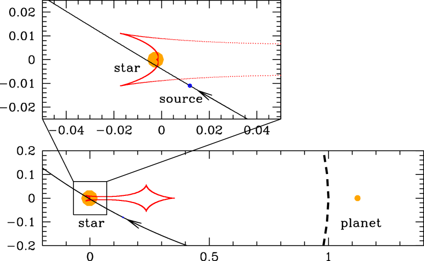
Figure 3: Geometry of the lens system responsible for the microlensing event MOA 2010-BLG-477. In the lower panel, the filled dots represent the locations of the host star and planet. The closed figure composed of concave curves represents the caustic. The curve with an arrow represents the source trajectory with respect to the caustic. The big dashed circle centered at the host star represents the Einstein ring. The upper panel shows the enlargement of the region enclosed by a small box in the lower panel. The small filled circle represents the source star where its size is scaled by the caustic size.

5.1 Constraints from Measurement of $\theta_{\rm E}$

The most important constraints on the lens mass and distance come from the measurement of $\theta_{\rm E}$, which can be rewritten from Equation (2) as

$$\theta_{\rm E}=\frac{\theta_{\star}}{\rho_{\star}}=\frac{\sqrt{F_{I}/(\pi S_{I})}}{\rho_{\star}}$$ (7)

where $F_{I}$ is the intrinsic (dereddened) flux of the source and $S_{I}$ is its intrinsic $I$-band surface brightness. A key point is that the surface brightness does not depend at all on the microlens model (just on the source color and/or spectrum). Hence, $\theta_{\rm E}$ depends on the model only through the parameter combination $\sqrt{f_{s}}/\rho_{\star}$, where $f_{s}$ is the instrumental source flux ($f_{s}=1$ corresponds to magnitude 18). It is clear from Table 1 that this parameter combination varies very little. The biggest uncertainties are therefore in measuring the surface brightness and measuring the offset between the instrumental flux $f_{s}$ and the dereddened source flux $F_{I}$. Traditionally, these are measured simultaneously by determining the offsets of the color and magnitude, respectively, of the source from the clump on an instrumental CMD (Yoo et al., 2004). An instrumental CMD from CTIO is shown in Figure 4. From it, we can read instrumental magnitude in $I$ of 19.07. The instrumental $V-I$ color is measured more accurately from a regression of $V$ flux vs. $I$ flux, and gives $-0.35$.

Comparing to the instrumental clump position, we find $(V-I)_{0}=0.55\pm 0.05$ and $I_{0}=17.61\pm 0.15$, assuming $[(V-I),I]_{0,\rm clump}=(1.06,14.42)$. The color error is determined empirically from a sample of microlensed dwarfs with spectra (Bensby et al., 2011), while the magnitude error comes primarily from the error in fitting the clump centroid and the assumed Galactocentric distance of 8 kpc (both about 0.1 mag). These lead to an estimate $\theta_{\star}=0.79\pm 0.06$.

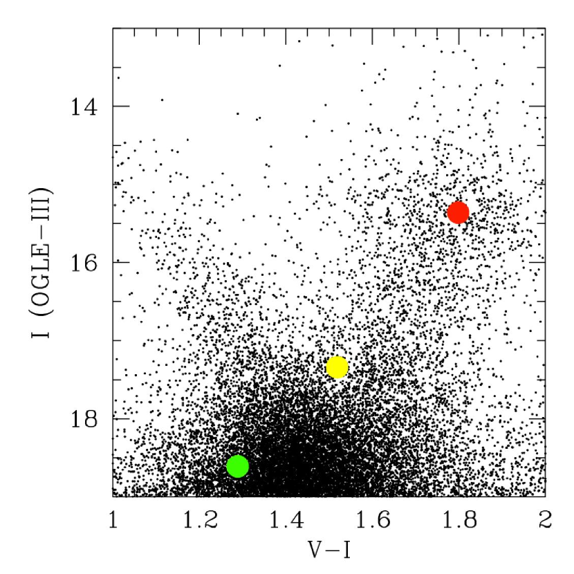
Figure 4: OGLE-III 8x8 arcmin calibrated color-magnitude diagram (CMD) in $I$- and $V$-band. The red, yellow and green solid circles mark the centroid of the red giant clump, the blend, and the source position, respectively.

We can compare the dereddened color estimate to the color deduced from the high-resolution spectrum reported in Section 2, from which we measured an effective temperature of $T=5950\pm 150\,$K, which corresponds to $(V-I)_{0}=0.65\pm 0.04$. These determinations are marginally consistent. We adopt the first to maintain the general practice of microlensing papers, but note that if we adopted the mean of the two estimates, the inferred value of $\theta_{\star}$ (and so $\theta_{\rm E}$) would rise by 2%.

Finally, we evaluate

$$\theta_{\rm E}=1.38\pm 0.11\,{\rm mas}$$ (8)

This value is unusually large and implies that the lens must be very massive or very close. Specifically

$$\frac{M}{M_{\odot}}\frac{\pi_{\rm rel}}{{\rm mas}}=\frac{\theta_{\rm E}^{2}}{\kappa\,M_{\odot}\,{\rm mas}}=0.233\pm 0.036$$ (9)

5.2 Constraints from Lens Flux Limits

The model gives a measurement of the light coming not only from the source, but also from any other stars in the same point spread function, generally called blended light. This light may come from the lens itself, a companion to the lens, a companion to the source, or any unrelated star on the same line of sight, but not participating to the amplification process.

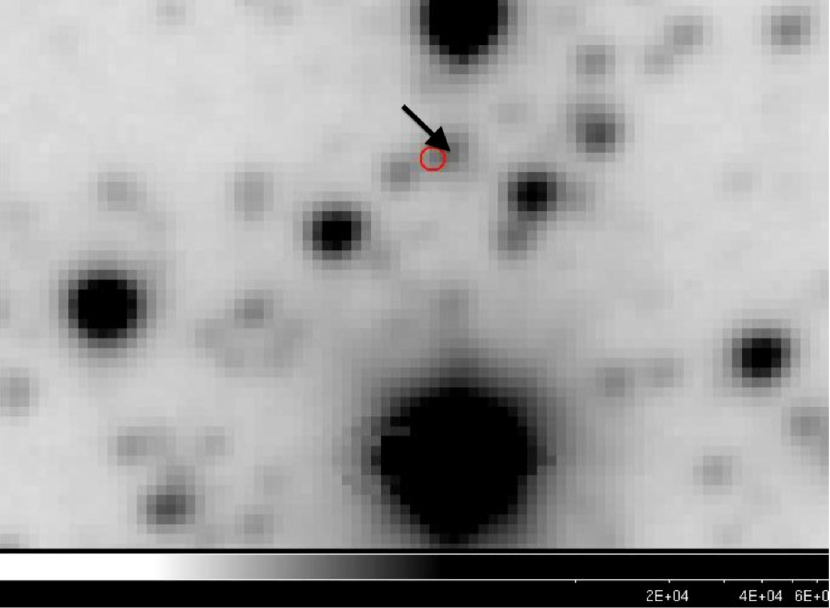
Figure 5: OGLE-III reference image of the BLG 176.8 field, in the region of our microlensed target. North is up and East to the left side. One pixel is $0.26\arcsec$. The red circle marks the position of the source (and the lens) from DIA analysis of CTIO images, in between two OGLE stars: the brighter of them (pointed at by a black arrow), at $0.37\arcsec$ from the source, corresponds in magnitude to the blended light measured by the model. The source is too faint to be detected in this crowded image.

The OGLE-III image of this field, displayed in Figure 5, shows two stars at the target position. Their $I$-band magnitudes in the OGLE-III photometric catalogue is $I=17.446\pm 0.052$ for the brighter star, numbered 119416, and $I=17.807\pm 0.059$ for the fainter one with number 119534. They are separated by $1.26\arcsec$, enough to be separated by PSF photometry at good sites such as CTIO or Las Campanas (OGLE) in Chile. A difference image analysis (DIA) made on CTIO images shows that the microlensed star does not correspond to the position of either star (red circle in Figure 5), but is displaced by 1 CTIO pixel ($0.37\arcsec$) from the brighter star.

Now, the blended light in $I$-band as measured from DoPhot CTIO photometry by the model is $I_{\rm b}=17.443\pm 0.031$, and this corresponds precisely to the flux from the brighter star among the two OGLE stars, which is not separated from the microlensed target at the scale of the CTIO seeing (typically $1\arcsec$). Knowing that the blended flux comes from an unrelated blended star, the light from the lens must be smaller. We can rigorously conclude that the lens has less than half the light in the observed blend. Otherwise, the lens and blend would be separated by at least $2\times 0.37^{\prime\prime}=0.74^{\prime\prime}$ in the OGLE image, and so would have been at least marginally resolved.

An additional argument showing that the lens is faint enough to remain undetected comes from its large relative proper motion ($10.3\pm 0.8$ mas/yr). DIA analysis of OGLE-III good seeing images separated by 3.3 years shows no residual at the target position, which proves that no detected star has moved during this period.

Combining this limit with Equation (9) yields strong constraints on the lens. The lens must be closer than the source, and so be at or closer than the Galactocentric distance, and suffer the same or less extinction. These imply $I_{\rm L,0}=I_{\rm b}-2.5\log(0.5)-A_{\rm I}>17.0$, and so $M_{I}>2.5$, which corresponds to $M<1.4\ M_{\odot}$ (Straižys & Kuriliene, 1981; Bessell & Brett, 1988). Then, even the $2\,\sigma$ limit from Equation (9) implies $\pi_{\rm rel}>0.10$ mas and so $D_{L}<4.4\,$kpc. But $I_{\rm L,0}>17.0$ then implies $M_{I}>3.8$, which corresponds to $M<1.0\,M_{\odot}$. Cycling through this argument one more time yields $D_{L}<3.7\,$kpc, $M_{I}<4.2$, $M<1\ M_{\odot}$. If the lens were in front of some of the dust, this argument would become still stronger. However, at the relatively high latitude of this field ($b=-5^{\circ}$), most of the dust probably lies in front of 3 kpc, and in any case, there is no basis for adopting a more optimistic assumption about the dust.

5.3 Constraints from the Microlens Parallax $\pi_{\rm E}$

Table 1 shows that parallax alone improves the fit by ${\Delta}{\chi^{2}}=8.6$, while including both parallax and lens orbital motion improves it by ${\Delta}{\chi^{2}}=54.4$. However, while detection of these effects is therefore unambiguous, we cannot fully disentangle one from the other. For each effect, one of its two parameters is well determined while the other is highly degenerate with one parameter from the other effect. As first discovered by Batista et al. (2011) and further analyzed by Skowron et al. (2011), weak detections of parallax and orbital motion lead to a strong degeneracy between $\pi_{\rm E,\perp}$ (the component of $\mbox{\boldmath$\pi$}_{\rm E}$ perpendicular to the projected position of the Sun) and $\omega$ (the component of orbital motion perpendicular to planet-star axis), while $\pi_{\rm E,\parallel}$ and $\dot{s}$ are well constrained. The impact of this is illustrated in Panel (a) of Figure 6, which shows $\chi^{2}$ values by color as a function of $(\pi_{\rm E,N},\pi_{\rm E,E})$.

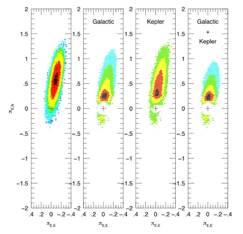
Figure 6: Parallax vector $(\pi_{\rm E,N},\pi_{\rm E,E})$ for the $u_{0}>0$ solution, from Markov Chain Monte Carlo fit to MOA-2010-BLG-477. Left panel (a) displays individual chain points, color-coded by $\Delta\chi^{2}$ (1, 4, 9, 16, 25, 36) for black, red, yellow, green, cyan, blue. Second panel (b) shows effect of weighting by the Galactic model, geometric Jacobian, and flux constraint. Lower parallaxes (and so higher masses) are heavily favored, except that too low parallaxes (corresponding to $M>1.0\,M_{\odot}$) are ruled out by the flux constraint. Third panel shows the effect of weighting using the Jacobian due to orbital motion parameters, which by itself disfavors the heaviest masses because these tend to imply unphysical orbits, but favors moderately high masses (see text). The final panel shows the effect of combining Galactic and Kepler priors.

First, it is clear that the parallax vector is almost completely degenerate along a line that is $8.4^{\circ}$ west of north, within $1^{\circ}$ of the predicted orientation of $\pi_{E,\perp}$ ($7.7^{\circ}$). Second, the light curve excludes $\pi_{\rm E}>1.3$ at $3\,\sigma$. As we have

$$\frac{M}{M_{\odot}}\times\pi_{\rm E}=\frac{\theta_{\rm E}}{\kappa\,M_{\odot}\,{\rm mas}}=0.169\pm 0.013$$ (10)

this corresponds to $M>0.13\,M_{\odot}$. Thus, combining constraints from this section and from Section 5.2, and using Equation (9), we have

$$0.13\,M_{\odot}<M<1.0\,M_{\odot};0.5\,{\rm kpc}<D_{L}<2.8\,{\rm kpc}$$ (11)

Note that, because the parallax contours pass through the origin, parallax provides no additional constraint at low $\pi_{\rm E}$, i.e., at high mass.

A similar diagram is given for the slightly disfavored $u_{0}<0$ solution in Figure 7.

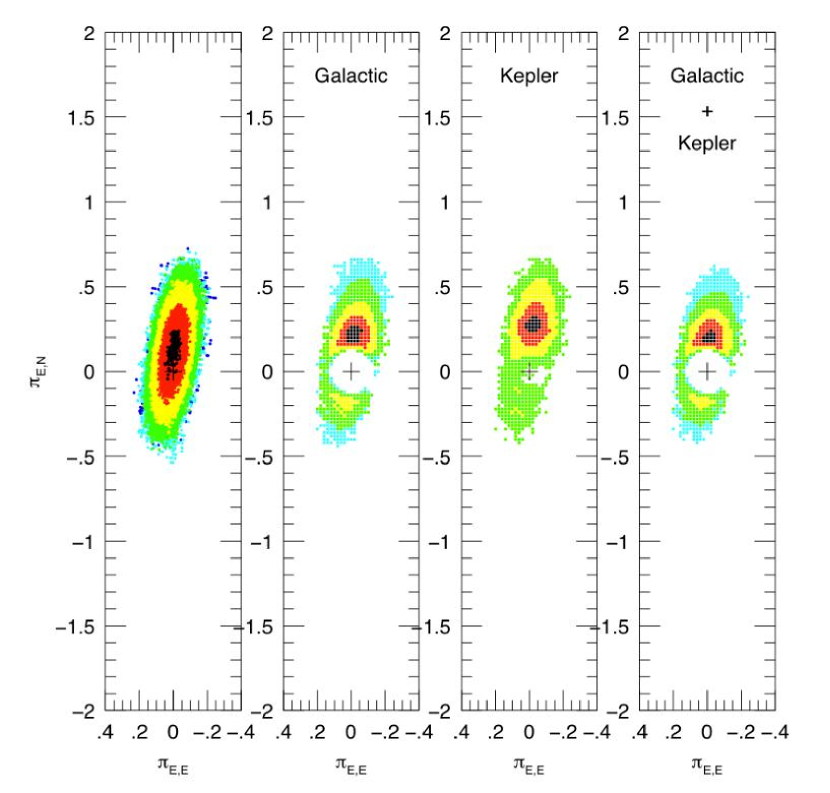
Figure 7: Parallax vector $(\pi_{\rm E,N},\pi_{\rm E,E})$ for the $u_{0}<0$ solution, from Markov Chain Monte Carlo fit to MOA-2010-BLG-477. See description of Figure 6 for details.

5.4 Post-Bayesian Analysis

Equation (11) defines the limits of what can be said rigorously about the lens mass and distance based on current data. As we discuss in Section 6, the lens could almost certainly be detected by high-resolution imaging, which would probably completely resolve the uncertainty in Equation (11). In the meantime, we can perform a Bayesian analysis based on a Galactic model and constraints from a Keplerian orbit. Figure 6 shows that each of these constraints separately favors small values of $\pi_{\rm E}$ and hence, relatively large masses and distances (within the limits set by Equation [11]), and so tend to reinforce each other. Panel (a) shows the raw results of the MCMC. Panel (b) shows the same chain, post-weighted by the Bayesian prior due to the Galactic model and the flux constraint. The latter, which implies $M<1.0\,M_{\odot}$ (Section 5.2) is responsible for the circular “holes” at the centers of panels (b) and (d). As discussed in detail by Batista et al. (2011) this includes terms not only reflecting the density of lenses along the sight and the expected distribution of proper motions, but also a Jacobian transforming from the “natural microlensing variables” to the physical system of the Galaxy. It is this last term that actually dominates, particularly in the “near field” ($D_{L}<2.8\,$kpc) permitted by the constraints, and is roughly $\sim D_{L}^{5}$ (Batista et al. (2011), Equation [18]). This weighting is so severe that one must ask whether the result of the weighting is plausibly compatible with the raw $\chi^{2}$ from the light curve. In this case, the solutions favored by the Bayesian post-weighting are compatible with the raw $\chi^{2}$ minimum at better than $2\,\sigma$, so there is no major conflict.

Panel (c) shows the results of post-weighting the chain only by the orbital Jacobian. This is described in detail by Skowron et al. (2011) for the case of chains with complete orbital solutions. These contain two orbital parameters (called $\gamma_{z}$ and $s_{z}$) in addition to the two first-order orbital parameters considered here ($\dot{s}$ and $\omega$). These higher order parameters would be completely unconstrained in the present problem, so we simply resample the chain with a uniform integration over these two parameters. Panel (c) clearly also favors more massive, more distant lenses (although not the most massive), but it is not immediately obvious why. Appendix E details the reasons behind this result. Finally, we note that, as expected, the combined effect of these two priors shown in Panel (d) is stronger than either separately.

Why do the Galactic model and Kepler constraints each favor more distant (and more massive lenses) than the light curve alone (see Fig. 6)? The Galactic model constraint is virtually guaranteed to favor more distant lenses because, as mentioned above, most of the weighting is simply due to a coordinate transformation from microlensing to physical coordinates, and there is more phase space at larger distances. Since the distance errors are fairly large, this effect will be relatively strong. By contrast, the Kepler constraint could have just as easily favored more-distant as less-distant lenses. The most likely explanation is then, simply, that the light curve prediction of the distance is too close by 1.7 sigma, and the constrained value (panel d) is a better estimate. This conjecture is testable by future observations, as described in the next section.

6 Future High Resolution Observations

Follow-up observations are important to check the predictions of our models. In the microlensing field, the idea of doing follow-up observations preceded the detection of planets, going back at least to 1998 in the case of MACHO-LMC-5, with the corresponding HST observations published in Alcock et al. (2001). Then, it was successfully applied to derive more accurate parameters of the planetary systems, using HST or adaptive optics systems at Keck or VLT, for instance in Bennett et al. (2006); Dong et al. (2009); Janczak et al. (2010); Batista et al. (2011); Kubas et al. (2012). In the future, it could be used to study planets in the habitable zones of nearby dwarf stars, as suggested by di Stefano & Night (2008); di Stefano (2012).

While the Bayesian analysis strongly favors a lens close to $1\,M_{\odot}$, i.e, the upper limit permitted by the measurements, there is no airtight evidence against lower-mass lenses. Fortunately, this question can almost certainly be resolved by high-resolution imaging. The $VIH$ source magnitudes are $V_{s}=19.98\pm 0.03$, $I_{s}=18.71\pm 0.03$, and $H_{s}=17.35\pm 0.03$. These come from CTIO $H$-band measurements, taken simultaneously with $I$ and $V$-band observations. A linear regression between both fluxes gives a very accurate instrumental color of $(I-H)_{\rm CTIO}=1.707\pm 0.002$. After converting $H$ to the 2MASS photometric system and $I$ to the OGLE-III system by use of common stars in the CTIO field, the color becomes $I-H=1.36\pm 0.03$. Subtracting this color from the $I$ magnitude of the source in the OGLE-III system ($18.71$) returns the above value for $H$.

As we now show, the lens brightness must be similar to the source brightness. As can be judged from Figure 5, the field is relatively sparse, at a Galactic latitude of $b=-5.095^{\circ}$, so these two stars (for the moment superposed) will very likely be the only two stars in their immediate high-resolution neighborhood.

Let us consider three examples consistent with Equation (9), $(M/M_{\odot},D_{L}/{\rm kpc})=(0.1,0.4)$, $(0.5,1.7)$, $(1.0,2.8)$. These would have lens absolute magnitudes $M_{H}=(9.6,6.0,3.4)$ according to Kroupa & Tout (1997) and so $H_{\rm L,0}=(17.6,17.1,15.6)$. Of course, the extinction would be different at these different distances, but the entire column to the source is only $A_{H}\sim 0.3$. Therefore, a 0.5 $M_{\odot}$ lens star will be as bright as the source, and even a lens star at the bottom of the main sequence will produce an easily detectable amount of light ($0.5$ mag) over the expected source magnitude.

Since all $M/D_{L}$ combinations produce similar $H$ magnitudes, such a measurement would, by itself, have little predictive power. But these various scenarios would yield substantially different $J-H$ colors, which would add discriminatory power. Time has been allocated on various large telescopes to observe the field of this event, detect and measure the light coming from the source and lens stars.

In addition, because of the relatively large proper motion, $\mu=10.3\pm 0.8$ mas/yr the lens and source could be separately resolved within about 5 years. This would then yield the angle of proper motion ($=\tan^{-1}(\pi_{\rm E,E}/\pi_{\rm E,N})$) and so (from Figure 6) the amplitude of $\pi_{\rm E}$ (Ghosh et al., 2004).

We can also consider follow-up observations with the Hubble Space Telescope, which will be able to detect the lens-source relative proper motion as early as 2012 (Bennett et al., 2007). The implied absolute magnitudes for the three examples given above ($M=0.1$, 0.5, and $1.0\,M_{\odot}$) are $M_{I}=(12.3,7.9,4.1)$, and the implied extinction free magnitudes are $I_{\rm L,0}=(20.3,19.1,16.3)$. Since the extinction in the foreground of the lens is $A_{I}<1.0$, this implies that the host star should be detectable with at least 9% of the $I$-band flux of the source star over the full range of main sequence host star masses.

Finally, the ESA satellite GAIA to be launched in 2013 will image the Galactic Bulge down to $V\sim 20$ mag, so it may detect the lensing object and will certainly measure its proper motion if it does.

In conclusion, these additional observations should reveal whether our choice of second-order effects (microlensing parallax and planet orbital motion) correspond to the reality. If we find contradictory results to our predictions, then it will be a strong argument to conduct the modeling of additional effects mentioned in Section 4.4, such as xallarap effect from a binary source, or involvement of a third body.

7 Final results, conclusions and perspectives

In order to select the best among the three competing models (standard, parallax only, orbital motion and parallax), a simple comparison of $\chi^{2}$ values is not enough, because more refined models use more parameters. Taking into account these additional parameters by normalizing the $\chi^{2}$ estimate by the number of degree of freedom is not the proper way to select the best model. A vast literature exists about model selection, and an application of different criteria to astrophysics is described in Liddle (2007). A simple way to take care of the larger number of parameters is to use the Akaike Information Criterion (AIC) (Akaike, 1974), which introduces a penalty to the $\chi^{2}$ by adding twice the number of additional parameters. Different criteria, such as the Bayesian Information Criterion (BIC) (Schwarz, 1978) or the Deviation Information Criterion, introduced by Spiegelhalter et al. (2002), can also be used. Formulas are given below, where $\Delta k$ is the number of additional parameters, $N$ the number of data points, and $\chi^{2}(\overline{\theta})$ the $\chi^{2}$ of the average parameter set $\overline{\theta}$.

$$\Delta{\rm AIC} = \Delta\chi^{2}+2\ \Delta k$$

$$\Delta{\rm BIC} = \Delta\chi^{2}+\Delta k\ \log N$$

$$\Delta{\rm DIC} = \Delta(2\ \overline{\chi^{2}}-\chi^{2}(\overline{\theta}))$$ (12)

As there are 7 parameters in the standard model, 9 in the parallax only model and 11 in the orbital motion and parallax model, we see that our observed difference in $\chi^{2}$ of 8.6 in the parallax only model is only marginally significant according to the AIC (the expected difference is 4), while the observed difference of 54.4 (for the $u_{0}>0$) or 50.7 (for the $u_{0}<0$) is clearly an improvement of the orbital motion and parallax model over the standard one (the expected difference is 8). Similar results are obtained using DIC, while the difference between models returned by BIC is less significant.

However, it is important to note that $\Delta k$ strictly corresponds to the number of additional parameters only in the case of a linear regression problem. Here, we clearly have non-linear fits, so we should compute an “effective” number of parameters, which is difficult to estimate. The above conclusion should therefore not be taken as a quantitative one.

A confirmation of the detection of second-order effects comes from the fact that in the orbital motion and parallax model, the degeneracy between $u_{0}<0$ and $u_{0}>0$ models is clearly broken. It is instructive to plot both second-order effects vs each other, separately for the $u_{0}<0$ and $u_{0}>0$ solutions. This is done in Figure 8, where the orbital motion $\gamma$ is plotted vs. the parallax effect $\pi_{\rm E}$.

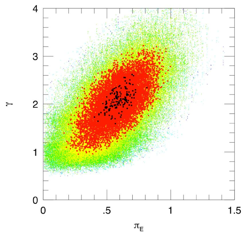
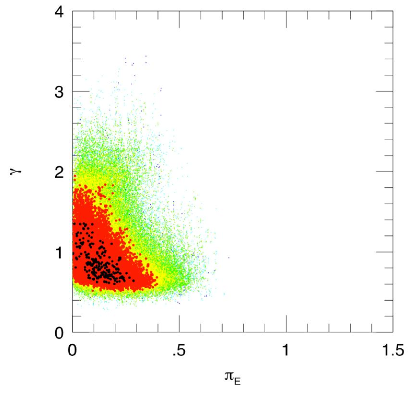
Figure 8: Variation of the orbital motion effect vs. the parallax effect for the orbital motion and parallax solutions. The left side corresponds to the $u_{0}>0$ solution, while the right side is for the $u_{0}<0$ solution.

If we remember that the ratio of the projected kinetic to potential energy must be smaller than 1 to get bound orbits, and that this ratio is proportional to $\gamma^{2}$, where the proportionality constant depends on $\pi_{\rm E}$ as given by Equation E3, it is easy to interpret these diagrams. When $\pi_{\rm E}$ increases, the proportionality factor decreases, so that if $\gamma$ remains small enough, the bound orbit condition is respected. In the $u_{0}>0$ diagram (left side), small values of $\pi_{\rm E}$ (say below 0.17) have a proportionality factor larger than 1. As $\gamma$ is nearly 1 for these solutions, they are ruled out, and the light curve confirms it, as few small $\chi^{2}$ solutions (black and red points) lie there. Larger $\pi_{\rm E}$ are also excluded, as they correspond to large $\gamma$ values, although the light curve would favor such solutions. The only surviving region in this diagram is around $\pi_{\rm E}\sim 0.35$, corresponding to lens masses of half a solar mass, where the proportionality factor is about 0.4 and $\gamma$ slightly exceeds 1.

In the $u_{0}<0$ diagram (right side), although this is slightly disfavored by the light curve ($\Delta\chi^{2}=6.7$ for the best chain without the circular orbit constraint), there is a region where $\gamma$ is about constant at 0.7 for $\pi_{\rm E}$ varying from 0 to 0.4. The bound solutions correspond to the larger values of the $\pi_{\rm E}$ domain (smaller proportionality factor), and they therefore agree with the range found in the $u_{0}>0$ diagram.

We therefore conclude that both solutions agree, and give bound orbits when the lens mass is about half solar, corresponding to a lens distance of about 1.6 kpc.

If we now move to the post-bayesian analysis, we see that this solution favored by the light curve has some tension with the Galactic model constraint, because nearby lenses are rarer than more distant ones. But if we move to more distant lenses, we get many chains with unbound orbits or high eccentricities. By the way, the $u_{0}>0$ solution, which has a lower $\chi^{2}$ than the alternate $u_{0}<0$ solution, is also the one where more chains correspond to unbound orbits.

There is therefore a tension between Galactic and Keplerian priors, and the issue will only be solved photometrically, by measuring the light coming from the source and the lens. This will be the subject of a forthcoming article about this event.

We conclude by giving the 1-D distributions of lens mass, lens distance, and planet orbit semi-major axis. The mass function for the lenses involved in these plots include main-sequence stars, brown dwarfs, but also white dwarfs, neutron stars and black holes, which may have large masses without violating the lens flux limit constraint. For the MS and BD stars, we adopt the following slopes of the present-day mass function $dN/d\ln(M)$: $-0.3$ between 0.03 and 0.7 $M_{\odot}$, $-1.0$ between 0.7 and 1.0 $M_{\odot}$, and $-4.0$ above. For the remnants, we adopt gaussian distributions, whose mean value, standard deviation, and fraction of total mass with respect to MS and BD stars below $1.0\ M_{\odot}$ are given in Table 2.

Table 2: Mass distribution of remnant stars (white dwarfs, neutron stars and black holes), with respect to main sequence stars and brown dwarfs below $1.0\ M_{\odot}$

Remnant	$<M>$	$\sigma$	ratio
WD	0.6	0.07	22/69
NS	1.35	0.04	6/69
BH	5.0	1.0	3/69

For details about the choice of these numbers, please refer to Gould (2000a).

In each diagram (see Figure 9 for mass and flux, and Figure 10 for distance and semi-major axis), the black curves show the full mass function, while the red curves show the mass function truncated at $1\ M_{\odot}$. For MS stars, this limit is imposed by the lens flux constraint, and will be refined once we obtain the adaptive optics photometry of the individual stars in the field. WD at this mass are extremely rare; Jovian planets around pulsars (NS) have not been found, despite very extensive searches; and super-Jupiter planets orbiting BH are a priori unlikely.

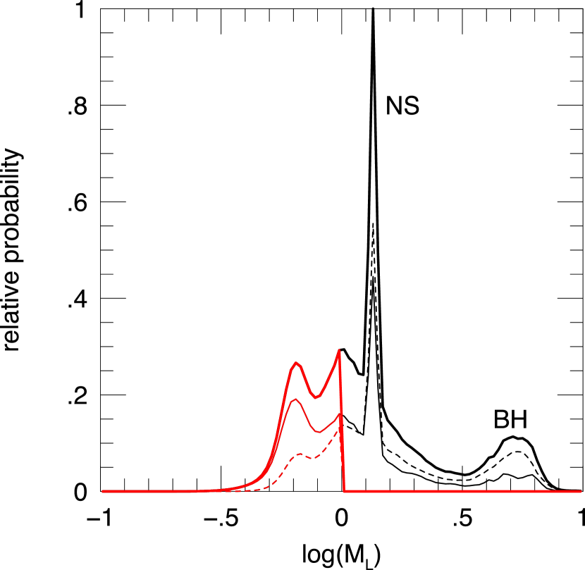
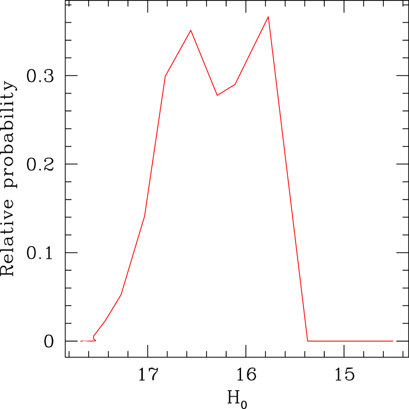
Figure 9: Distribution of lens mass and lens flux in $H$-band (from left to right) computed from the post-bayesian analysis. In the left diagram, the black curves show the full mass function, while the red curves show the mass function truncated at $1\ M_{\odot}$. The solid curves represent the $u_{0}>0$ solution, while the dashed curves correspond to the $u_{0}<0$ one. The bold solid curves are the sum of the two other curves. In the right diagram, the curve corresponds to the red bold solid curve of the mass distribution.

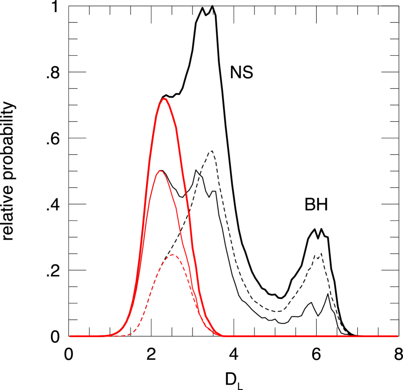
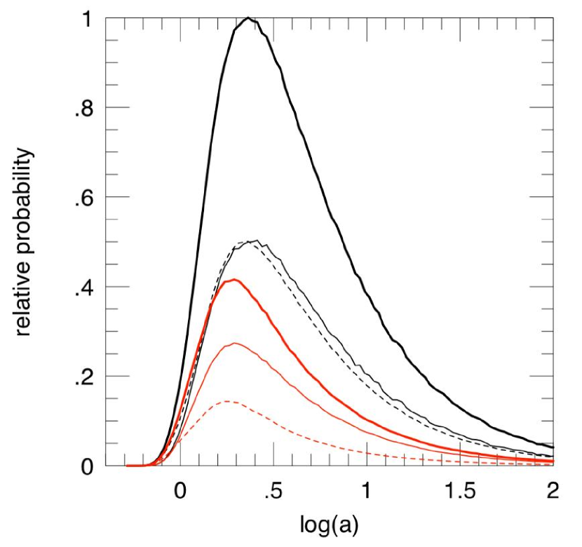
Figure 10: From left to right: distribution of lens distance (in kpc) and semi-major axis of the planet orbit (in AU), computed from the post-bayesian analysis. For details, see the description of Figure 9.

Let us first consider the lens mass distribution: the no-flux-limit (black) curve shows a huge spike at expected NS position and a smaller bump corresponding to BH. Note that for these bumps, the $u_{0}<0$ solution dominates, despite its $\chi^{2}$ handicap. This is because the Galactic model very strongly favors distant lenses, primarily because of the volume factor, and this overwhelms the modest preference of the light curve for nearby lenses. Because $\theta_{\rm E}$ is roughly fixed, these distant lenses are massive. This preference is much stronger in the $u_{0}<0$ solution, which can be seen in its rapid rise beginning at $\log M=-0.3$. Note that the WD peak (at $\log M=-0.22$) is clearly visible, especially in the $u_{0}>0$ solution.

The lens distance distribution basically looks at this same situation from the standpoint of distance. The new notable feature is that both MS and NS peaks are in the disk, while the BH bump is in the Bulge. And the semi-major axis distribution peaks at about 2-3 AU.

¿From these diagrams, we can estimate a most probable value of lens mass, distance and semi-major axis, and an asymmetric standard deviation read at 50% of the distribution corresponding to the red bold curves. We get a star and planet mass of $M_{*}=0.67^{+0.33}_{-0.13}\ M_{\odot}$ and $m_{p}=1.5^{+0.8}_{-0.3}\ M_{\rm JUP}$, respectively, at a distance of $D=2.3\pm 0.6$ kpc, and with a semi-major axis of $a=2^{+3}_{-1}$ AU.

As a final note, it could be said that more complex models are worth exploring: the geometry of the caustic crossing, where the source passes close to the three-cusps tail of the caustic, is extremely sensitive to a third body (second planet or binary companion to the lens star). A similar geometry where two planets were detected is described in Gaudi et al. (2008); Bennett et al. (2010). These models could be investigated in a forthcoming paper, once we get the lens flux measurement from adaptive optics.

Appendix A Observations at Dome C

ASTEP 400 is a 40cm Newtonian telescope installed at the Concordia base, located on the Dome C plateau in Antarctica (Daban et al., 2011). Although the aim of the project concerns transiting planets, the ability to observe near-continuously during the antarctic winter and the excellent weather on site (Crouzet et al., 2010) imply that the telescope can usefully complement microlensing observations from other sites, even though the declination of the fields and their crowding make the analysis difficult.

The observations with ASTEP 400 started on August 12, 2010, 15:27 UT after the first alert was sent by email and phone to Concordia. On August 14, 23:59 UT, the observations were stopped because the magnification had become too small for useful observations. The weather conditions were excellent. However, the seeing conditions were poor ( 3-4”), mostly due to the low-declination of the field and location of the telescope on the ground. The 229MB of data corresponding to 500x500 cropped images were transmitted to Nice through satellite connexion around August 17-18 for an in-depth analysis.

Although the data of this run were not good enough for being used in this study, this pioneering test will serve for improving the thermics of the acquisition system and get higher quality future observations of microlensing targets.

Appendix B Difference Image Analysis using pySIS

The pySIS3.0 difference image analysis package is fully described in Albrow et al. (2009). It is based on the original ISIS package (Alard & Lupton, 1998; Alard, 2000) but the kernel used to transform the reference image to the current image before subtraction is no longer analytic, but numerical. This allows dealing with images whose PSF cannot be assimilated to a sum of gaussian profiles. The numerical kernel has been introduced in image subtraction by Bramich (2008). One of the regular problems encountered in difference image analysis is the choice of the best possible reference image. For astrometry, the best seeing image is generally a good choice, if the sky background is not too high. For photometry, it is our experience that stacking good images improves the result, but only if these images have been acquired during a short time slot, to avoid light variations of the target and slow variations due for instance to small changes in the flat-field. In order to choose good reference images, we use a suite of Astromatic software (Bertin, 2011), namely SExtractor and PSFex. SExtractor builds catalogues of sources from all images of a given telescope, with their characteristics, and PSFex derives a model of the PSF of these images, from which we extract a few numbers to estimate the image quality (seeing, ellipticity, number of stars). This allows an almost automatic selection of the templates, with a final verification by eye to check the selected images.

Once the images have been subtracted using these templates, the photometry of the target is done by iteratively centering the PSF on the light maximum close to the center of the image. This method enables the photometering of faint stars in the glare of nearby much brighter stars.

Appendix C Noise Model and Error Rescaling

The standard procedure of rescaling error bars so that the $\chi^{2}/{\rm dof}$ of each telescope data set is of order unity is acceptable if the resulting error bars roughly correspond to the dispersion of the data points at a given time for this data set. There is therefore an interplay between finding the correct model and rescaling the error bars, because a too large rescaling factor reduces the constraint from a given data set and allows the model to shift from the correct one. Our procedure has been to use rescaling factors which look plausible given the telescope size and site quality, trying to get a $\chi^{2}/{\rm dof}$ of order unity only if the dispersion in successive data points is well reproduced by this rescaling scheme. This generally involves two parameters to modify the original photometric error bars $e_{\rm ori}$. One is a minimal error $e_{\rm min}$ to reproduce the dispersion of very bright (or in this case, highly magnified) sources due to fundamental limitations of the photometry, such as flat fielding errors. The other is the classical multiplicative rescaling factor $f$. The adopted formula is:

$$e=f\sqrt{e_{\rm ori}^{2}+e_{\rm min}^{2}}$$ (C1)

The balance between both rescaling factors is given by comparing the cumulative distribution of $\chi^{2}/{\rm dof}$, ordered from magnification given by the model, to a standard cumulative distribution for gaussian errors. An example for OGLE and MOA distributions is given in Figure 11. Table 3 gives the adopted values of both parameters for each telescope. It must also be noted that for some amateur telescopes, data were binned before this rescaling process. Finally, after the initial modeling was conducted, it was realized that three data sets could not accommodate the condition $\chi^{2}/{\rm dof}\sim 1$ (Auckland and VLO) or a positive source flux (Perth). They were therefore removed and the final models are based on 16 data sets.

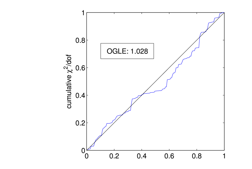
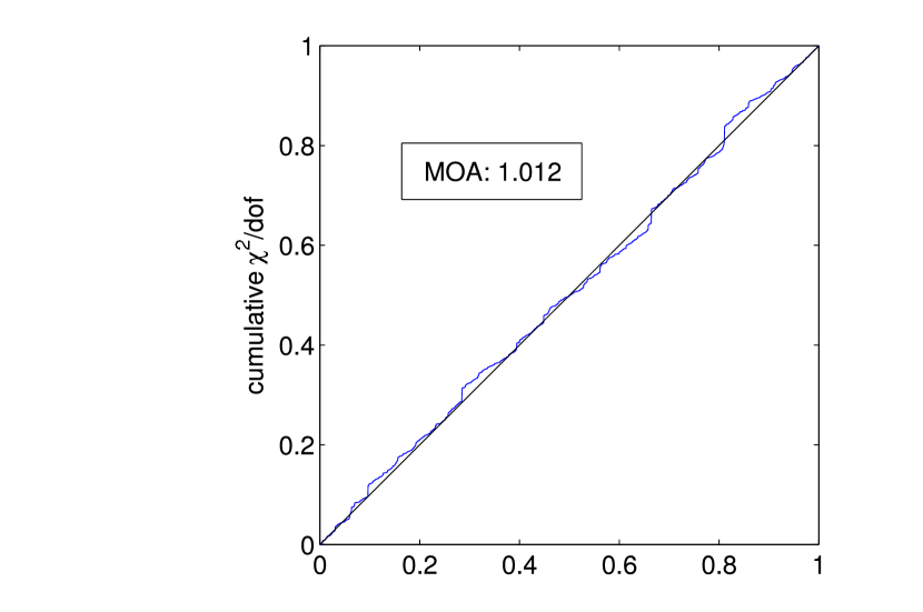
Figure 11: Cumulative $\chi^{2}$/dof distribution for rescaled error bars in the case of OGLE photometry (left) and MOA photometry (right).

Appendix D Detailed Treatment of Limb-darkening Corrections

It is generally difficult to treat the limb-darkening effect accurately, because it varies from one telescope data set to the other, primarily due to the different photometric bands involved. Second-order effects include hardware-specific variations of the spectral response (filters, CCDs), and for very broad bands, the atmospheric and interstellar extinctions. We adopt the linear limb-darkening approximation using the formalism given by Equation 4, introduced by Albrow et al. (1999) and An et al. (2002). This is a common formalism in the microlensing community, but the more widely used formalism is based on the following equation

$$I_{\lambda}(\cos{\phi})=I_{\lambda}(1)\times\left[1-u_{\lambda}(1-\cos{\phi})\right]$$ (D1)

where $I_{\lambda}(1)$ is the specific intensity at disk center and $u_{\lambda}$ is the linear limb-darkening coefficient. We compute the values of $u_{\lambda}$ from a stellar atmosphere model from the Kurucz ATLAS9 grid (Kurucz, 1993) using the method described by Heyrovský (2007). As we converted the $u_{\lambda}$ values to our LDC parameter $\Gamma_{\lambda}$, we give the $u_{\lambda}$ values in Table 3, and recall the conversion relation

$$\Gamma_{\lambda}=\frac{2\,u_{\lambda}}{3-u_{\lambda}}$$ (D2)

Table 3: Data description for each telescope

Observatory	Band	$u_{\lambda}$ (uncor.)	$u_{\lambda}$ (ext. cor.)	Binning	N	$f$	$e_{\rm min}$	Photometry
OGLE	$I$	0.4399	0.4363		157	2.4	0.010	OGLE DIA
CTIO	$I$	0.4395	0.4375		133	1.5	0.010	DoPhot
CTIO	$V$	0.5931	0.5908		21	2.0	0.015	DoPhot
Auckland	W12	0.5016	0.4843	Y	5	1	0.003	DoPhot
FCO	unfiltered	0.5550	0.5150	Y	4	1.7	0.003	DoPhot
FTS	$i^{\prime}$	0.4547	0.4524		68	3.0	0.002	pySIS
Kumeu	W12	0.5016	0.4852	Y	17	3.5	0.003	DoPhot
Perth	$I$	0.4325	0.4297		26	3.0	0.003	pySIS
FTN	$i^{\prime}$	0.4547	0.4524		72	3.8	0.006	DanDIA
Possum	W12	0.5204	0.5031		77	5.4	0.003	pySIS
SAAO	$I$	0.4261	0.4217		2364	2.2	0.003	pySIS
SAAO	$V$	0.6114	0.6086		3	1.2	0.003	pySIS
VLO	unfiltered	0.5442	0.5022	Y	3	1	0.003	DoPhot
Wise	unfiltered	0.5522	0.5131	Y	9	0.8	0.003	DoPhot
Canopus	$I$	0.4355	0.4335		50	1.5	0.010	pySIS
Danish	$I$	0.4394	0.4370		167	2.2	0.003	pySIS
MOA	red	0.4754	0.4694		3985	1.05	0	MOA DIA
LT	$i^{\prime}$	0.4543	0.4513		41	4.7	0	DanDIA
Monet N	$I$	0.4414	0.4392		130	4.3	0.004	pySIS

Note. — a: This data set was not used in the final models

For the source characteristics, we adopt the spectroscopic result ($T_{\rm eff}=6000$ K, $\log g=4.0$, [Fe/H]=0.0). We thus get an estimate of the limb-darkening effect for each data set. Table 3 shows the adopted values of $u_{\lambda}$ for each individual telescope and band combination, both with and without interstellar extinction correction, together with the final number of data points after rejection of possible outliers, and details about the image reduction process. As can be seen, these coefficients vary even if the photometric band is supposedly the same. See for instance the Cousins $I$-band and SDSS $i^{\prime}$-band, or the Wratten #12 filter (W12) used at some amateur telescopes to mimic an $R$ band. More details about the derivation of these values for each telescope can be found in Heyrovský (2007); Fouqué et al. (2010); Muraki et al. (2011).

We have also computed the effect of interstellar extinction on the LDCs, as it is not a priori negligible: we typically find differences of a few $10^{-3}$ for a data set with a filter and a few $10^{-2}$ for unfiltered ones. The magnitude of the effect could then be neglected for filtered data sets, but not for unfiltered ones or very broad band filters. To give an idea, we compare its effect to the uncertainty of our spectroscopic determination of the effective temperature of the source, about 150 K. For the OGLE $I$-band, the difference between LDCs with and without interstellar extinction correction for an adopted extinction of 1.2 mag corresponds to a shift in effective temperature of 40 K, while for the Possum broad W12 filter, it corresponds to about 200 K, and for an unfiltered data set, it gives a shift of about 500 K.

Appendix E Detailed analysis of the Kepler constraint

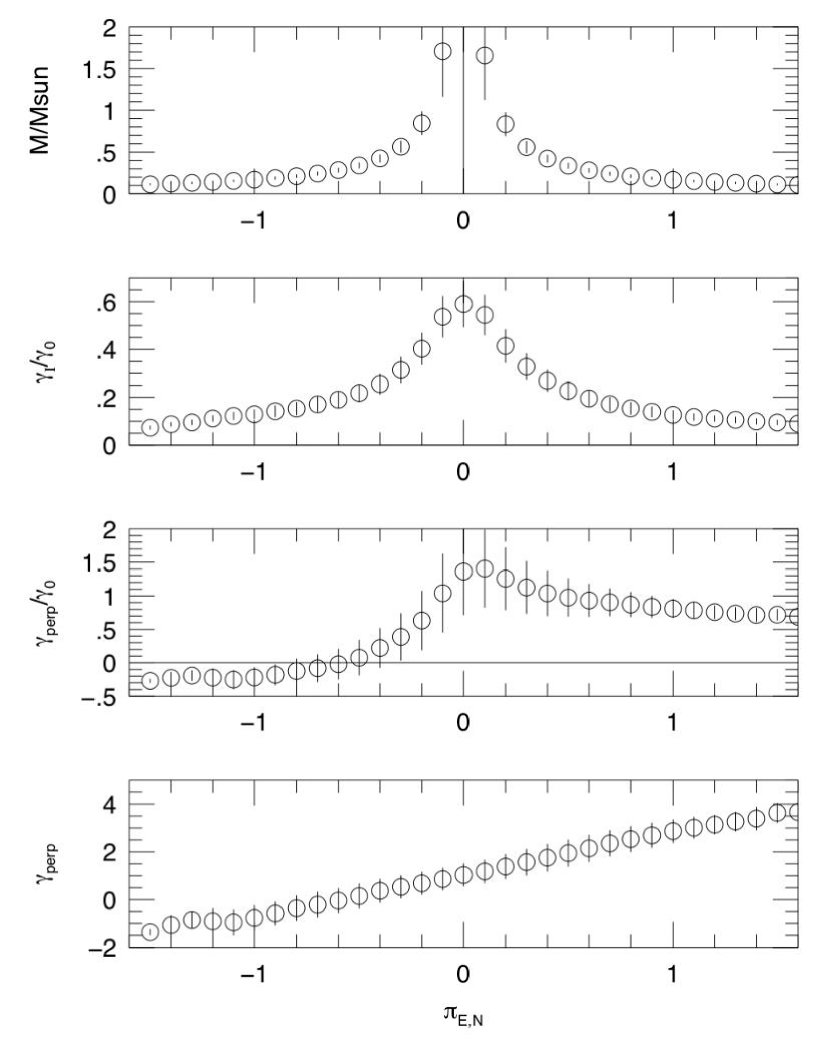
Figure 12: Binned lens characteristics as a function of MCMC variable $\pi_{\rm E,N}$. Bottom panel shows that $\pi_{\rm E,N}$ is highly correlated with $\gamma_{\perp}$, the component of orbital motion perpendicular to the projected planet-star axis, as found earlier by Batista et al. (2011). This is responsible for the poor determination of $\pi_{\rm E,N}$ in Figure 6(a). Top panel: highest masses are associated with low $\pi_{\rm E,N}$. Third panel: these are disfavored because $\gamma_{\perp}/\gamma_{0}$ tends to saturate its physical limit (unity). Second panel: relatively high masses (with $\pi_{\rm E,N}<0$) are favored because $\gamma_{\parallel}/\gamma_{0}$ (as well as $\gamma_{\perp}/\gamma_{0}$) hover near 0.5, a value favored by the virial theorem.

Figure 12 shows several quantities plotted against $\pi_{\rm E,N}$. In each case the mean and standard deviation of all chain links within a given $\pi_{\rm E,N}$ bin are calculated. The bottom panel shows the behavior of $\omega$ ($=\gamma_{\perp}$). Since $\pi_{\rm E,N}$ is very similar to $\pi_{\rm E,\perp}$, this reflects the degeneracy between the perpendicular components of Earth orbital motion (parallax) and lens orbital motion, which is analyzed in some detail by Batista et al. (2011) and Skowron et al. (2011). In the present case, the correlation is quite tight. The top panel shows the lens mass $M=\theta_{\rm E}/\kappa\pi_{\rm E}$. Since $\theta_{\rm E}$ is nearly constant for different links in the chain, the mass scales $M\sim\pi_{\rm E}^{-1}$ and so is peaked near $\pi_{\rm E,N}=0$ where $\pi_{\rm E}$ is near its minimum (see Figure 6).

It is the two middle panels that enable one to understand why the orbital Jacobian favors relatively high masses. These show, respectively $\gamma_{\parallel}/\gamma_{0}$ and $\gamma_{\perp}/\gamma_{0}$, where

$$\gamma_{\parallel} = s^{-1}\ \dot{s},$$ (E1)

$$\gamma_{\perp} = \omega,$$ (E2)

$$\gamma_{0}^{2} = \frac{8\pi^{2}}{\kappa\,s^{3}\pi_{\rm E}}\,\theta_{\rm E}\,\biggl{(}\pi_{\rm E}+\frac{\pi_{\rm s}}{\theta_{\rm E}}\biggr{)}^{3}$$ (E3)

Note that $(\gamma_{\perp}^{2}+\gamma_{\parallel}^{2})/\gamma_{0}^{2}$ is the ratio of the so-called projected kinetic to projected potential energy, which has a strict upper limit of unity for bound orbits. We do enforce this limit, but the main impact of the orbital motion is more subtle. First look at $\gamma_{\perp}/\gamma_{0}$. In the region away from $\pi_{\rm E,N}\sim 0$, we have both $\gamma_{0}\propto\pi_{\rm E}$ (Equation E3) and (very roughly) $\gamma_{\perp}\propto\pi_{\rm E}$ (bottom panel). Hence, $\gamma_{\perp}/\gamma_{0}$ is approximately constant in these two regimes. Much of the $\pi_{\rm E,N}>0$ region is at or above the physical limit $\gamma_{\perp}=\gamma_{0}$, which is why these values are disfavored in Figure 6(c).

Now examine $\gamma_{\parallel}/\gamma_{0}$. By itself, $\gamma_{\parallel}$ does not vary much with $\pi_{\rm E,N}$, so the form of the structure is basically just $\gamma_{0}^{-1}$, which scales $\propto\pi_{\rm E,N}^{-1}$ away from zero. The point is, however, that the overall scale (which is set by the measurement of $\gamma_{\parallel}$) is small, so that except near $\pi_{\rm E,N}\sim 0$, $\gamma_{\parallel}/\gamma_{0}$ is extremely close to zero. Naively, this would seem to be disfavored by the virial theorem, but how does the Jacobian “know” about this? For simplicity of exposition let us consider circular orbits. For these, $\gamma_{\parallel}/\gamma_{0}=0$ implies that the planet is exactly in the plane of the sky: either the orbit is exactly face-on (so this is always true), or the orbit just happens to be passing through the plane of the sky at the time of the event peak. The Jacobian is “unhappy” about either alternative because there is very little Kepler-parameter space relative to chain-variable space at such orbital configurations.

Finally, note that in the immediate neighborhood of $\pi_{\rm E,N}\sim 0$ (where $M$ reaches its highest values), $\gamma_{\perp}$ is frequently at or above its physical limit ($\gamma_{0}$), which is exacerbated by the relatively high values of $\gamma_{\parallel}$. This is reponsible for the modest suppression of extremely low parallaxes (high masses) in Figure 6. Thus, both Kepler and Galactic+flux priors separately predict a relatively high lens mass, near the limit of what is permitted by the flux constraint.

References

- Abe et al. (2004) Abe, F., et al. 2004, Science, 305, 1264
- Akaike (1974) Akaike, H. 1974, IEEE T. Automat. Contr., 19, 716
- Alard (2000) Alard, C. 2000, A&A, 144, 363
- Alard & Lupton (1998) Alard, C., & Lupton, R.H. 1998, ApJ, 503, 325
- Albrow et al. (1999) Albrow, M.D., et al. 1999, ApJ, 522, 1022
- Albrow et al. (2000) Albrow, M.D., et al. 2000, ApJ, 534, 894
- Albrow et al. (2009) Albrow, M.D., et al. 2009, MNRAS, 397, 2009
- Alcock et al. (2001) Alcock, C., et al. 2001, Nature, 414, 617
- An et al. (2002) An, J.H., et al. 2002, ApJ, 572, 521
- Batista et al. (2011) Batista, V., et al. 2011, A&A, 529, A102
- Beaulieu et al. (2006) Beaulieu, J.-P., et al. 2006, Nature, 439, 437
- Bennett (2008) Bennett, D.P. 2008, in Exoplanets, ed. J. Mason, Berlin: Springer, ISBN: 978-3-540-74007-0 (arXiv:0902.1761)
- Bennett (2010) Bennett, D.P. 2010, ApJ, 716, 1408
- Bennett & Rhie (1996) Bennett, D.P., & Rhie, S.-H. 1996, ApJ, 472, 660
- Bennett et al. (2006) Bennett, D.P., et al. 2006, ApJ, 647, L171
- Bennett et al. (2007) Bennett, D.P., Anderson, J., & Gaudi, B.S. 2007, ApJ, 660, 781
- Bennett et al. (2008) Bennett, D.P. et al. 2008, ApJ, 684, 663
- Bennett et al. (2010) Bennett, D.P., et al. 2010, ApJ, 713, 837
- Bensby et al. (2011) Bensby, T., et al. 2011, ApJ, in press
- Bertin (2011) Bertin, E. 2011,
- Bessell & Brett (1988) Bessell, M.S., & Brett, J.M. 1988, PASP, 100, 1134
- MOA: Bond et al. (2001) Bond, I. A., et al. 2001, MNRAS, 327, 868
- Bramich (2008) Bramich, D.M. 2008, MNRAS, 386, L77
- Cassan et al. (2012) Cassan, A. et al. 2012, Nature, 481, 167
- Claret (2000) Claret, A. 2000, A&A, 363, 1081
- Crouzet et al. (2010) Crouzet, N., et al. 2010, A&A, 511, 36
- Daban et al. (2011) Daban, J.-B., et al. 2011, SPIE 7733, 151
- di Stefano & Night (2008) di Stefano, R., & Night, C. 2008, arXiv:0801.1510
- di Stefano (2012) di Stefano, R. 2012, arXiv:1112.2366
- Dominik (1998) Dominik, M. 1998, A&A, 349, 108
- Dong et al. (2006) Dong, S., et al. 2006 ApJ, 642, 842
- Dong et al. (2009) Dong, S., et al. 2009 ApJ, 695, 970
- Dominik et al. (2010) Dominik, M., et al. 2010, Astron. Nachr., 331, 671
- Fouqué et al. (2010) Fouqué, P., et al. 2010, A&A, 518, A51
- Gaudi et al. (2008) Gaudi, B.S., et al. 2008, Science, 319, 927
- Gaudi (2010) Gaudi, B.S. 2010, in Exoplanets, ed. S. Seager, Tucson: University of Arizona Press, 79 (arXiv:1002.0332)
- Ghosh et al. (2004) Ghosh, H., et al. 2004, ApJ, 615, 450
- Gould (1992) Gould, A. 1992, ApJ, 392, 442
- Gould et al. (1994) Gould, A., Miralda-Escude, J., & Bahcall, J.N. 1994, ApJ, 413, L105
- Gould (1994) Gould, A. 1994, ApJ, 421, L71
- Gould (2000a) Gould, A. 2000a, ApJ, 535, 928
- Gould (2000b) Gould, A. 2000b, ApJ, 542, 785
- Gould (2008) Gould, A. 2008, ApJ, 681, 1593
- Gould et al. (2006) Gould, A., et al. 2006, ApJ, 644, L37
- Gould et al. (2010) Gould, A., et al. 2010, ApJ, 720, 1073
- Griest & Safizadeh (1998) Griest, K., & Safizadeh, N. 1998, ApJ, 500, 37
- Han (2009) Han, C. 2009, ApJ, 691, 452
- Heyrovský (2007) Heyrovský, D. 2007, ApJ, 656, 483
- Ioka et al. (1999) Ioka, K., Nishi, R., Kan-Ya, Y. 1999, Prog. Theor. Phys., 102, 983
- Janczak et al. (2010) Janczak, J., et al. 2010, ApJ, 711, 731
- Kennedy et al. (2007) Kennedy, G.M., Kenyon, S.J., & Bromley, B.C. 2007, Ap&SS, 311, 9
- Kennedy & Kenyon (2008) Kennedy, G.M., & Kenyon, S.J. 2008, ApJ, 673, 502
- Kroupa & Tout (1997) Kroupa, P., & Tout, C. 1997, MNRAS, 287, 402
- Kubas et al. (2012) Kubas, D., et al. 2012, A&A, 540, A78
- Kurucz (1993) Kurucz CD-ROM 13, ATLAS9 Stellar Atmosphere Programs and 2 km/s grid (Cambridge: SAO)
- Lecar et al. (2006) Lecar, M., Podolak, M., Sasselov, D., & Chiang, E. 2006, ApJ, 640, 1115
- Liddle (2007) Liddle, A.R. 2007, MNRAS, 377, L74
- Lissauer (1987) Lissauer, J.J. 1987, Icarus, 69, 249-265
- Lissauer (1993) Lissauer, J.J. 1993, ARA&A, 31, 129
- Mao & Paczyński (1991) Mao, S. & Paczyński, B. 1991, ApJ, 374, L37
- Milne (1921) Milne, E.A. 1921, MNRAS, 81, 361
- Miyake et al. (2012) Miyake, N., et al. 2012, ApJ, submitted
- Muraki et al. (2011) Muraki, Y. et al. 2011, ApJ, 741, 22
- Nemiroff & Wickramasinghe (1994) Nemiroff, R.J., & Wickramasinghe, W.A.D.T. 1994, ApJ, 421, L21
- Paczyński (1986) Paczyński, B. 1986, ApJ, 304, 1
- Pejcha & Heyrovský (2009) Pejcha, O., & Heyrovský, D. 2009, ApJ, 690, 1772
- Penny et al. (2011) Penny, M.T., Mao, S., & Kerins, E. 2011, MNRAS, 412, 607
- Poindexter et al. (2005) Poindexter, S., et al. 2005, ApJ, 633, 914
- Rattenbury et al. (2002) Rattenbury, N.J., Bond, I.A., Skuljan, J., & Yock, P.C.M. 2002, MNRAS, 335, 159
- Rhie et al. (2000) Rhie, S. H., et al. 2000, ApJ, 533, 378
- Schwarz (1978) Schwarz, G. 1978, Ann. Stat., 5, 461
- Skowron et al. (2011) Skowron, J., et al. 2011, ApJ, 738, 87
- Spiegelhalter et al. (2002) Spiegelhalter, D.J., Best, N.G., Carlin, B.P., van der Linde, A. 2002, J.R. Statist. Soc. B, 64, 583
- Straižys & Kuriliene (1981) Straižys, V., & Kuriliene, G. 1981, Ap&SS, 80, 353
- Sumi et al. (2003) Sumi, T., et al. 2003, ApJ, 591, 204
- Sumi et al. (2010) Sumi, T., et al. 2010, ApJ, 710, 1641
- Sumi et al. (2011) Sumi, T., et al. 2011, Nature, 473, 349
- Tsapras et al. (2009) Tsapras, Y., et al. 2009, Astron. Nachr., 330, 4
- Vermaak (2000) Vermaak, P. 2000, MNRAS, 319, 1011
- OGLE: Udalski (2003) Udalski, A. 2003, Acta Astron., 53, 291
- Witt & Mao (1994) Witt, H.J., & Mao, S. 1994, ApJ, 429, 66
- Witt & Mao (1995) Witt, H.J., & Mao, S. 1995, ApJ, 447, L105
- Yoo et al. (2004) Yoo, J., et al. 2004, ApJ, 603, 139