Refraction and Diffraction of Waves in Electromagnetic (Photonic) Crystals Formed by Anisotropically Scattering Elements

Abstract

Refraction and diffraction of waves in natural crystals and artificial crystals formed by anisotropically scattering centers are considered. A detailed study of the electromagnetic wave refraction in a two-dimensional photonic crystal formed by parallel threads is given by way of example. The expression is derived for the effective amplitude of wave scattering by a thread (in a crystal) for the case when scattering by a single thread in a vacuum is anisotropic. It is established that for a wave with orthogonal polarization, unlike a wave with parallel polarization, the index of refraction in crystals built from metallic threads can be greater than unity, and Vavilov-Chrernkov radiation becomes possible in them. The set of equations describing the dynamical diffraction of waves in crystals is derived for the case when scattering by a single center in a vacuum is anisotropic.

Because a most general approach is applied to the description of the scattering process, the results thus obtained are valid for a wide range of cases without being restricted to either electromagnetic waves or crystals built from threads.

Introduction

Creation of metamaterials has recently become an area of vigorous research worldwide. The so-called electromagnetic (photonic) crystals built from, e.g., metallic split rings or parallel metallic threads [1], including threads with dimensions within the nanometer range [2] are actively being studied. Such photonic crystals can be used, and are already being used, for solving various tasks, particularly in antenna microwave technology [1]. In addition, crystals built from periodically strained parallel metallic threads can serve as resonators in volume free electron lasers (VFEL) [3, 4, 5].

The interaction of electromagnetic waves with photonic crystals is accompanied by the phenomena of refraction and diffraction. As is known, the refractive index of the medium formed by randomly distributed scatterers is related to the amplitude of scattering by a single center as follows [6]

$$n^{2}=1+\frac{4\pi\rho}{k^{2}}A(0),$$ (1)

where $\rho$ is the density of scatterers, $A(0)$ is the amplitude of forward scattering.

However, it is shown in [7, 8] that if scatterers are located periodically (e.g. crystal), then for a correct description of the refraction process, one should use a modified expression for $n^{2}$

$$n^{2}=1+\frac{4\pi}{k^{2}\Omega_{3}}\frac{A}{1+ikA},$$ (2)

where $\Omega_{3}$ is the volume of the unit cell of the crystal. If scattering by a single centers is elastic, formula (2), in contrast to (1), leads to a physically correct result: the imaginary part of the refractive index equals zero. Note that (2) is derived under the assumption that scattering by a single center is isotropic, i.e., the amplitude $A$ is independent of the scattering angle. In the present paper, refraction of waves in crystals built from anisotropically scattering centers is considered. Metallic threads are the simplest example of such scatterers: scattering by such threads of electromagnetic waves with the electric-field vector polarized orthogonally to the thread axis is anisotropic for all wavelengths [9, 10].

This paper is arranged as follows: Section 1 gives a detailed analysis of a nonplane waves scattering by a single thread. Section 2 describes the method used for finding the refractive index by the example of crystals formed by isotropic scatterers. Section 3 considers the case of crystals formed by anisotropic scatterers.

1 Scattering of Electromagnetic Waves with Orthogonal Polarization by Thread

1.1 Plane Wave

Before we start to consider scattering of a cylindrical wave by a thread (cylinder), let us recall the case of a plane wave. Assume, as usual, that the radius $R$ of the thread is much smaller than its length $L$, and so in analytical treatment, the thread can be considered infinitely long.

The solution to the problem of diffraction of a plane electromagnetic wave by an infinite cylinder can be found in the form of a series over Bessel and Hankel functions [11]. Let a wave with perpendicular polarization (vector $\vec{E}$ is perpendicular to the axis of a cylinder) be scattered by a cylinder placed in a vacuum (Fig.1). The axis of the cylinder coincides with the $z$-axis of the rectangular coordinate system. Let us also introduce a cylindrical coordinate system $(r,\varphi,z)$, as is shown in Fig.1.

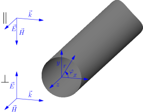
Figure 1: Diffraction of a plane electromagnetic wave by a cylinder.

For simplicity, we shall consider the case when the wave vector $\vec{k}$ is perpendicular to the axis of the cylinder. Then the field of the scattered wave can be written in the form [11]:

$$\begin{split}\vec{H}_{e}&=\vec{e}_{z}\sum\limits_{n=-\infty}^{\infty}i^{n}c_{n}^{\perp}H_{n}(kr)e^{-in\varphi},\\ \vec{E}_{e}&=\frac{ic}{\omega}\sum\limits_{n=-\infty}^{\infty}i^{n}c_{n}^{\perp}\left[\vec{e}_{r}\frac{-in}{r}H_{n}(kr)-\vec{e}_{\varphi}kH_{n}^{\prime}(kr)\right]e^{-in\varphi},\end{split}$$ (3)

where the coefficients $c_{n}^{\perp}$ are calculated by the formula

$$c_{n}^{\perp}=\frac{-J_{n}(k_{2}R)J^{\prime}_{n}(kR)+\frac{1}{\sqrt{\varepsilon}}J_{n}^{\prime}(k_{2}R)J_{n}(kR)}{J_{n}(k_{2}R)H_{n}^{(1)^{\prime}}(kR)-\frac{1}{\sqrt{\varepsilon}}J_{n}^{\prime}(k_{2}R)H_{n}^{(1)}(kR)}.$$ (4)

Here $J_{n}$ is the Bessel function of order $n$, $H_{n}$ is the Hankel function of the first kind of order $n$, $k_{2}=k\sqrt{\varepsilon}$, $\varepsilon$ is the dielectric permittivity of the thread (for metals, $\varepsilon=1+4\pi\sigma i/\omega$, where $\omega$ is the frequency of the electromagnetic field, $\sigma$ is the conductivity, and the magnetic permittivity $\mu$ is assumed to be equal to 1), vectors $\vec{e}_{r}$, $\vec{e}_{\varphi}$, $\vec{e}_{z}$ are the unit vectors of the cylindrical coordinate system, and the amplitude of the incident wave is assumed to be equal to 1.

Considering the limits of Bessel and Hankel functions of small argument, one can find that for a perfectly conducting cylinder, the relationships $c_{0}^{\perp}\approx-c_{\pm 1}^{\perp}$ and $c_{0}^{\perp}\gg c^{\perp}_{n}$ hold for all $|n|>1$ at $kR\ll 1$. If a cylinder is not a perfect conductor, then the first equality is violated, but the absolute values of the coefficients $c_{0}^{\perp}$ and $c_{\pm 1}^{\perp}$ remain comparable. What is more, if the dielectric permittivity of a cylinder is $\varepsilon-1\sim 1$, then $c_{0}^{\perp}\ll c_{\pm 1}^{\perp}$. Thus, at $kR\ll 1$, in (3), it suffices to take account of only the terms $n=0$ and $n=\pm 1$. Note here that in considering a wave with parallel polarization in the long-wave limit, $c_{0}^{\parallel}\gg c_{n}^{\parallel}$ for all $n\neq 0$, and so in the series for the field, one can take account of the term $n=0$ alone.

Returning to our problem, let is recall that the two equations (3) are related through Maxwell’s equations, and so the second equation can readily be obtained from the first one by formula $\vec{E}_{e}=\frac{ic}{\omega}\mathop{\mathrm{rot}}\nolimits\vec{H}_{e}$. With thus eliminated electric field and with due account of the above remarks concerning the values of the coefficients $c_{n}$ (it is further assumed that $kR\ll 1$), one can write the scattered wave in the form:

$$\vec{H}_{e}=\vec{e}_{z}\Psi_{sc}=\vec{e}_{z}\left\{c_{0}H_{0}(kr)+2ic_{1}H_{1}(kr)\cos\varphi\right\},$$ (5)

where the superscript $\perp$ on the expansion coefficient is dropped.

If a plane wave $\vec{H}_{0}=\Psi_{0}\vec{e}_{z}=e^{ikx}\vec{e}_{z}$, is scattered by a cylinder placed at the origin of coordinates, then the total wave field is expresses as a sum of the field of the incident and scattered waves, i.e.,

$$\Psi=\Psi_{0}+\Psi_{sc}=e^{ikx}+c_{0}H_{0}(kr)+2ic_{1}H_{1}(kr)\cos\varphi.$$ (6)

Using the asymptotic expression for Hankel functions of large argument and the integral representation of Hankel functions, the above expression can be presented in the following form, provided $kr\gg 1$:

$$\Psi=e^{ikx}+A(\varphi)\int\limits_{-\infty}^{\infty}\frac{e^{ik\sqrt{r^{2}+z^{2}}}}{\sqrt{r^{2}+z^{2}}}\mathrm{d}z,$$ (7)

where $A(\varphi)=-\frac{i}{\pi}(c_{0}+2c_{1}\cos\varphi)=A_{0}+A_{1}\cos\varphi$.

Similarly to a three-dimensional case, by $A(\varphi)$ one should understand the amplitude of scattering of an electromagnetic wave by a thread at an angle $\varphi$ [12].

It should be noted that in contrast to a diverging spherical wave that characterizes scattering in a three-dimensional case, in a two-dimensional case, a diverging cylindrical wave is formed.

In view of (6), one can readily write the expression for the field in the case when the axis of a cylinder lies not in the origin of coordinates, but at point $\vec{r}_{1}$

$$\Psi=\Psi_{0}+\Psi_{sc}=e^{i\vec{k}\vec{r}}+e^{i\vec{k}\vec{r}_{1}}\cdot A_{0}i\pi H_{0}(k|\vec{r}-\vec{r}_{1}|)-e^{i\vec{k}\vec{r}_{1}}\cdot A_{1}\pi H_{1}(k|\vec{r}-\vec{r}_{1}|)\cos(\vec{k},\vec{r}-\vec{r}_{1}).$$ (8)

1.2 Cylindrical wave

Let now a cylindrical wave $\Psi_{0}=H_{0}(kr)$, diverging from the origin of coordinates, be incident onto this scatterer, which is placed at point $\vec{r}_{1}$. To analyze the scattering process in this case, one can decompose a cylindrical wave into elementary plane waves, which are scattered according to a well-known law (8). For the Hankel function, in particular, one can use the following representation:

$$H_{0}(kr)=\frac{1}{\pi}\int\limits_{-\infty}^{\infty}\frac{e^{i\vec{k}\vec{r}}}{\sqrt{k^{2}-k_{y}^{2}}}dk_{y}=\frac{1}{\pi}\int\limits_{-\infty}^{\infty}\frac{e^{i\vec{k}\vec{r}}}{\sqrt{k^{2}-k_{x}^{2}}}dk_{x}.$$ (9)

For the purposes of this paper, we do not need to know the exact decomposition, suffice it to know that the wave $\Psi_{0}=H_{0}(kr)$ can be presented as a sum of plane waves as follows: $H_{0}(kr)=\int f(k,k_{y})e^{i\vec{k}\vec{r}}dk_{y}$, or $H_{0}(kr)=\int f(k,k_{x})e^{i\vec{k}\vec{r}}dk_{x}$, where $k\equiv|\vec{k}|=const$ and $f(k,k_{y})$ is a certain function.

Thus, by decomposing the initial wave and in view of (8), one can immediately write the expression for a scattered wave

$$\Psi_{sc}=\int\limits_{-\infty}^{\infty}f(k,k_{y})e^{i\vec{k}\vec{r}_{1}}A_{0}i\pi H_{0}(k|\vec{r}-\vec{r}_{1}|)dk_{y}-\int\limits_{-\infty}^{\infty}f(k,k_{y})e^{i\vec{k}\vec{r}_{1}}A_{1}\pi H_{1}(k|\vec{r}-\vec{r}_{1}|)\cos(\vec{k},\vec{r}-\vec{r}_{1})dk_{y}.$$ (10)

Because $A_{0,1}$ and $H_{0,1}(k|\vec{r}-\vec{r}_{1}|))$ are only dependent on the absolute value of the wave vector $k$ and independent of $k_{y}$, they can be removed from the integration sign. Then, according to (9), the first integral in (10) equals $H_{0}(kr_{1})$, and (10) can be rewritten in the form:

$$\Psi_{sc}=H_{0}(kr_{1})\cdot A_{0}i\pi H_{0}(k|\vec{r}-\vec{r}_{1}|)-A_{1}\pi H_{1}(k|\vec{r}-\vec{r}_{1}|)\cdot I_{1},$$ (11)

where

$$I_{1}=\int\limits_{-\infty}^{\infty}f(k,k_{y})e^{i\vec{k}\vec{r}_{1}}\cos(\vec{k},\vec{r}-\vec{r}_{1})dk_{y}.$$ (12)

To evaluate the integral $I_{1}$, let us represent the cosine of the angle between vectors $\vec{k}$ and $\vec{r}-\vec{r}_{1}$ in the form: $\cos(\vec{k},\vec{r}-\vec{r}_{1})=\frac{\vec{k}(\vec{r}-\vec{r}_{1})}{k|\vec{r}-\vec{r}_{1}|}$. Then we have

$$I_{1}=\frac{\vec{r}-\vec{r}_{1}}{k|\vec{r}-\vec{r}_{1}|}\cdot\frac{1}{\pi}\int\limits_{-\infty}^{\infty}\vec{k}f(k,k_{y})e^{i\vec{k}\vec{r}_{1}}dk_{y}=\\ =-i\frac{\vec{r}-\vec{r}_{1}}{k|\vec{r}-\vec{r}_{1}|}\cdot\mathop{\mathrm{grad}}\nolimits_{1}\int\limits_{-\infty}^{\infty}f(k,k_{y})e^{i\vec{k}\vec{r}_{1}}dk_{y}=-i\frac{\vec{r}-\vec{r}_{1}}{k|\vec{r}-\vec{r}_{1}|}\cdot\mathop{\mathrm{grad}}\nolimits_{1}H_{0}(kr_{1}),$$ (13)

where the subscript “1” on the gradient symbol means that differentiation is performed with respect to the coordinates of the point $\vec{r_{1}}$. The differentiation yields $\mathop{\mathrm{grad}}\nolimits_{1}H_{0}(kr_{1})=-H_{1}(kr_{1})\frac{k\vec{r}_{1}}{r_{1}}$, and then

$$I_{1}=iH_{1}(kr_{1})\frac{\vec{r}_{1}(\vec{r}-\vec{r_{1}})}{r_{1}|\vec{r}-\vec{r_{1}}|}=iH_{1}(kr_{1})\cos(\vec{r}_{1},\vec{r}-\vec{r}_{1}).$$ (14)

The above yields that the total wave field for scattering of a cylindrical wave has the form:

$$\Psi=H_{0}(kr)+A_{0}i\pi H_{0}(kr_{1})\cdot H_{0}(k|\vec{r}-\vec{r}_{1}|)-A_{1}\pi iH_{1}(kr_{1})\cdot H_{1}(k|\vec{r}-\vec{r}_{1}|)\cos(\vec{r}_{1},\vec{r}-\vec{r}_{1}).$$ (15)

At large distances from the origin of coordinates ($kr_{1}\gg 1$), one can use the serial expansion $iH_{1}(z)\approx H_{0}(z)\left(1+\frac{i}{4z}\right)$. Substitution of this expression into (15) gives

$$\Psi=H_{0}(kr)+A_{0}i\pi H_{0}(kr_{1})\cdot H_{0}(k|\vec{r}-\vec{r}_{1}|)-A_{1}\pi H_{0}(kr_{1})\left(1+\frac{i}{4kr_{1}}\right)\cdot H_{1}(k|\vec{r}-\vec{r}_{1}|)\cos(\vec{r}_{1},\vec{r}-\vec{r}_{1}).$$ (16)

Comparing this equation with (8), one can conclude that with increasing distance between the origin of coordinates (the central point of the diverging cylindrical wave) and the scatterer, the difference between the amplitudes of scattering of cylindrical and plane waves by a thread diminishes, as might be expected.

Let us briefly consider the case when the initial cylindrical wave has the form $\Psi_{0}=H_{1}(kr)\cos\varphi$. By reasoning along the same lines, we obtain similar formulas, except for the expression for the integral $I_{1}$. Now it equals

$$I_{1}^{\prime}=-i\frac{\vec{r}-\vec{r}_{1}}{k|\vec{r}-\vec{r}_{1}|}\cdot\mathop{\mathrm{grad}}\nolimits_{1}H_{1}(kr_{1})\cos\varphi_{1}.$$ (17)

Now differentiation yields the following expression

$$\mathop{\mathrm{grad}}\nolimits_{1}H_{1}(kr_{1})\cos\varphi_{1}=\left\{kH_{0}(kr_{1})-\frac{2}{r_{1}}H_{1}(kr_{1})\right\}\cos\varphi_{1}\cdot\frac{\vec{r}_{1}}{r_{1}}+\frac{1}{r_{1}}H_{1}(kr_{1})\vec{e}_{x},$$ (18)

where $\vec{e}_{x}$ is the unit vector of the $x$-axis. The expression for a scattered wave will now have the form:

$$\Psi=\Psi_{0}+\Psi_{sc}=H_{1}(kr)\cos\varphi+\left\{A_{0}H_{1}(kr_{1})\cos\varphi_{1}\right\}i\pi H_{0}(k|\vec{r}-\vec{r}_{1}|)-\\ -\left\{A_{1}\cos\varphi_{1}\left(-iH_{0}(kr_{1})+\frac{2i}{kr_{1}}H_{1}(kr_{1})\right)\right\}\pi H_{1}(k|\vec{r}-\vec{r}_{1}|)\cos(\vec{r}_{1},\vec{r}-\vec{r}_{1})-\\ -\left\{\frac{-iA_{1}}{kr_{1}}H_{1}(kr_{1})\right\}\pi H_{1}(k|\vec{r}-\vec{r}_{1}|)\cos(\vec{r}-\vec{r}_{1},\vec{e}_{x}).$$ (19)

A particular case when the scatterer is placed on the $y$-axis, i.e., $\varphi_{1}=\pm\frac{\pi}{2}$, seems to be of interest. Here we have $\cos\varphi_{1}=0$, and the expression for a scattered wave simplifies appreciably:

$$\Psi_{sc}=\frac{i\pi A_{1}}{kr_{1}}H_{1}(kr_{1})H_{1}(k|\vec{r}-\vec{r}_{1}|)\cos(\vec{r}-\vec{r}_{1},\vec{e}_{x}).$$ (20)

It should be noticed that here the scattered wave does not vanish despite the zero amplitude of the incident wave at the scatterer location: $\Psi_{0}(\vec{r}_{1})=H_{1}(kr_{1})\cos\varphi_{1}=0$. Though there is not any paradox because at $\varphi_{1}=\pm\frac{\pi}{2}$, only the magnetic-field vector equals zero, $\vec{H}_{0}=\Psi_{0}\vec{e}_{z}$, while the electric-field vector has the form: $\vec{E}_{0}=\frac{ic}{\omega}\mathop{\mathrm{rot}}\nolimits\vec{H}_{0}=-\frac{ic}{\omega r_{1}}H_{1}(kr_{1})\vec{e}_{y}$, i.e., is nonzero. Thus, when $\varphi_{1}=\pm\frac{\pi}{2}$, only the electrical component of the initial wave is scattered by the thread.

2 Refraction of Waves in Photonic Crystals Formed by Isotropically Scattering Elements

Let us consider an infinite, two-dimensional crystal composed of periodically arranged scatterers. A well-known example of such a crystal is a photonic crystal built from parallel metallic threads [3], Fig. 2.

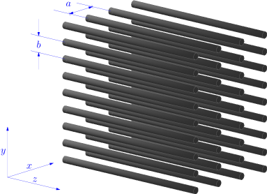
Figure 2: Crystal made of parallel metallic threads

For definiteness (but without loss of generality!), we shall consider such a crystal. Let the coordinates of the threads in the lattice be $(x_{mn},y_{mn})=(ma,nb)$, where $a$ and $b$ are the lattice spacings, $m$ and $n$ are the integers; the axes of the treads are parallel to the $z$-axis of the rectangular coordinate system.

One should distinguish between the cases when vector $\vec{E}$ of the incident wave is polarized parallel to the threads and when it is polarized perpendicular to them. In the first case, scattering at $kR\ll 1$ is isotropic and $A(\varphi)=A_{0}$, while in the second case, scattering is anisotropic even at $kR\ll 1$, and the amplitude has the above described angular dependence: $A=A_{0}+A_{1}\cos\varphi$. Certainly, when $kR\gtrsim 1$, in expression (6) one needs to retain more terms in the expansion (3), and the angular dependence of the amplitude can take a more complicated form.

In this section, we shall assume that scattering by the centers is isotropic with the amplitude $A_{0}$. Let us suppose that an electromagnetic wave $\sim e^{iqx}$ propagates in a crystal in the positive direction of the $x$-axis. This wave results from the summation of diverging cylindrical waves $i\pi H_{0}(k|\vec{r}-\vec{r}_{mn}|)$ radiated by all the threads. The amplitude of these waves has the form $\Phi=\Phi_{0}e^{iqx_{mn}}$, where $\Phi_{0}$ is independent of the position of the thread in the crystal. Using the method described in [14], let us find the relation between the wave numbers $k$ and $q$. Let us assume that the local field at the location of each thread is a sum of all waves coming from all other threads. Particularly, the local filed acting on the thread placed at the origin of coordinates ($m=n=0$) can be written as follows:

$$\Psi_{loc}=\Phi_{0}i\pi\sum\limits_{(m,n)\neq(0,0)}e^{iqx_{mn}}H_{0}(kr_{m,n})=\Phi_{0}i\pi\sum\limits_{(m,n)\neq(0,0)}e^{iqam}H_{0}\left(k\sqrt{(am)^{2}+(bn)^{2}}\right).$$ (21)

Since scattering is isotropic, all these waves are scattered by this thread with a known amplitude, equal to the amplitude $A_{0}$ of scattering of a plane wave by the thread, producing a diverging cylindrical wave with the amplitude $\Phi_{0}$:

$$\Phi_{0}=A_{0}\Psi_{loc}=A_{0}i\pi\Phi_{0}\sum\limits_{(m,n)\neq(0,0)}e^{iqam}H_{0}\left(k\sqrt{(am)^{2}+(bn)^{2}}\right).$$

We thus come to the dispersion equation for finding $q$

$$\frac{1}{A_{0}i\pi}=\sum\limits_{(m,n)\neq(0,0)}e^{iqam}H_{0}\left(k\sqrt{(am)^{2}+(bn)^{2}}\right)i=S(k,q).$$ (22)

The sum in (22) is taken as described in [14], and here we only give the resulting expression:

$$S(k,q)=-1-i\cdot\left\{\frac{2}{\pi}\left(\log\frac{kb}{4\pi}+C\right)+\frac{2}{kb}\frac{\sin ka}{\cos ka-\cos qa}+\frac{2}{b}\sum\limits_{n\neq 0}\frac{1}{k_{x}^{(n)}}\frac{\sin k_{x}^{(n)}a}{\cos k_{x}^{(n)}a-\cos qa}-\frac{b}{2\pi|n|}\right\},$$ (23)

where $k_{x}^{(n)}=i\sqrt{(2\pi n/b)^{2}-k^{2}}$, $C\approx 0.5772$ is the Euler constant. Let us assume that the scattering amplitude is sufficiently small: $|A_{0}(k)|\ll 1$ and the refractive index is close to unity: $|n-1|=|q/k-1|\ll 1$.

One can easily demonstrate that in this case, the second term between the braces is a dominating term, and far from the diffraction conditions ($ka\neq\pi n$) it can be presented in the form:

$$\frac{2}{kb}\frac{\sin ka}{\cos ka-\cos qa}\simeq\frac{4}{k^{2}ba}\cdot\frac{1}{n^{2}-1}=\frac{4}{k^{2}\Omega_{2}}\cdot\frac{1}{n^{2}-1},$$ (24)

where $\Omega_{2}=ab$ is the crystal unit cell area. We thus come to the following dispersion equation:

$$\frac{1}{A_{0}i\pi}\approx-1-\frac{4i}{k^{2}\Omega_{2}}\cdot\frac{1}{n^{2}-1},$$

from this we get

$$n^{2}=1+\frac{4\pi}{k^{2}\Omega_{2}}\cdot\frac{A_{0}}{1+i\pi A_{0}}.$$ (25)

At this point, it should be mentioned that the same result was obtained in [3] in a different way. In the case of elastic scattering (e.g. perfectly conducting threads), formula (25) gives a real value of the refractive index. This is easily verified by the optical theorem. It will be recalled that the optical theorem relates the imaginary part of the forward scattering amplitude to the total scattering cross section: $\mathop{\mathrm{Im}}\nolimits A(0)=\frac{k\sigma}{4\pi}$. For a two-dimensional case, the differential scattering cross section is related to the scattering amplitude as follows: $\frac{d\sigma}{d\varphi}=\frac{2\pi}{k}|A(\varphi)|^{2}$.

One can arrive at the same result using a slightly different method: start with the consideration of scattering of a plane wave by a one-dimensional grating built from threads and then proceed to the case of infinite crystals. As this method is more convenient for the purposes of the analysis given in the following section, let us also describe it here.

Let a plane wave be scattered by a one-dimensional array of scatterers, as is shown in Fig.  3.

Figure 3: Diffraction of a plane wave by a one-dimensional array of scatterers

The scattered wave in this case is a sum of cylindrical waves of the same amplitude $F$, which are radiated by each thread

$$\Psi_{sc}(x,y)=F\sum\limits_{n=-\infty}^{\infty}i\pi H_{0}(k\sqrt{x^{2}+(y-bn)^{2}}).$$

But the amplitude $F$ of the plane-wave scattering by a thread in the presence of other scatterers differs from the amplitude $A_{0}$ of scattering by a single thread. With the help of the general methods used for describing multiple scattering [6], the amplitude $F$ can be expressed in terms of $A_{0}$ as follows:

$$F=A_{0}+A_{0}F\sum\limits_{n\neq 0}i\pi H_{0}(kb|n|).$$ (26)

The physical meaning of equations (26) is obvious: there are two waves scattered by each thread (particularly, by the thread placed at the origin of coordinates): the plane wave $e^{ikx}$ and the wave $\Psi^{\prime}=F\sum\limits_{n\neq 0}i\pi H_{0}(kb|n|)$ scattered by all other threads with the amplitude $A_{0}$. The sum (26) is taken in [14]

$$S_{1}=\sum\limits_{n\neq 0}H_{0}(kb|n|)=\frac{2}{kb}-1-i\frac{2}{\pi}\left(C+\log\frac{kb}{4\pi}\right)-\frac{2i}{b}\sum\limits_{n\neq 0}\left(\frac{1}{\sqrt{(2\pi n/b)^{2}-k^{2}}}-\frac{b}{2\pi|n|}\right).$$ (27)

It is still assumed that $A_{0}\ll 1$, then using (26) and (27), one can derive the following expression for the effective scattering amplitude:

$$F=\frac{A_{0}}{1-i\pi S_{1}A_{0}}\simeq\frac{A_{0}}{1+i\pi A_{0}-i\frac{2\pi}{kb}A_{0}}.$$ (28)

Thus the wave field resulting from scattering of a plane wave by a one-dimensional grating has the form: [3, 9]

$$\Psi=e^{ikx}+F\sum\limits_{n=-\infty}^{\infty}i\pi H_{0}(k\sqrt{x^{2}+(y-bn)^{2}})\approx e^{ikx}+\frac{2i\pi}{kb}Fe^{ik|x|},$$ (29)

where $F$ is defined from (28), and is a sum of the wave fields of the plane wave incident onto the grating and the wave scattered by the grating. The scattered wave propagates in the positive direction of the $x$-axis at $x>0$, and in the negative direction at $x<0$, its amplitude in both cases being $\frac{2i\pi}{kb}F$. This quantity can be treated as the ”amplitude of scattering” of a plane wave by a grating built from threads.

Now let us consider the propagation of waves in a crystal formed by an infinite periodic system of plane gratings regularly spaced at an interval $a$ and composed of threads. Use the same method as before to derive the dispersion equation. The wave incident onto the grating placed at the origin of coordinates is a sum of waves scattered by all other gratings. Assuming that the amplitude of these waves has the form $\Phi=\Phi_{0}e^{iqam}$ with $\Phi_{0}$ being independent of the coordinates due to the periodicity of crystals, one can write the following expression

$$\Phi_{0}=\frac{2i\pi}{kb}F\sum\limits_{m\neq 0}\Phi_{0}e^{iqam}e^{ika|m|},$$

from which one can derive the dispersion equation (compare with (22))

$$1=\frac{2i\pi}{kb}F\sum\limits_{m\neq 0}e^{iqam}e^{ika|m|}.$$ (30)

The sum in (30) can easily be calculated using the geometric progression sum formula, and is equal to

$$\sum\limits_{m\neq 0}e^{iqam}e^{ika|m|}=-1-i\frac{\sin ka}{\cos ka-\cos qa}\simeq-1-\frac{2i}{ka}\cdot\frac{1}{n^{2}-1}.$$

By substituting the obtained value into equation (30) and using (28), we get the already known result

$$n^{2}=1+\frac{4\pi}{k^{2}\Omega_{2}}\cdot\frac{A_{0}}{1+i\pi A_{0}}.$$

Note here that similar consideration of a three-dimensional crystal case gives a well-known formula (2).

3 Refraction of Waves in Crystals. The Case of Anisotropic Scatterers

Assume now that the scattering amplitude has the form $A=A_{0}+A_{1}\cos\varphi$, i.e., scattering is anisotropic. Let us use the approach described in the previous section to consider the propagation of plane waves in a crystal composed of anisotropic scatterers.

Let a plane wave having the amplitude $e^{ikx}$ be incident onto a one-dimensional grating composed of anisotropically scattering centers (Fig. 3). Knowing how a cylindrical wave is scattered by such scatterers (see (15), (19)), one can determine that the angular dependence of the amplitude $F(\varphi)$ of scattering by each thread in the presence of other threads is the same as that of the amplitude $A(\varphi)$ of scattering by a single thread $F(\varphi)=F_{0}+F_{1}\cos\varphi$. The system of equations for finding $F_{0}$ and $F_{1}$ has the form (see (15) and (20)):

$$F_{0} = A_{0}+A_{0}F_{0}\sum\limits_{m\neq 0}i\pi H_{0}(kb|m|),$$ (31)

$$F_{1} = A_{1}+A_{1}F_{1}\sum\limits_{m\neq 0}i\pi H_{1}(kb|m|)\cdot(kb|m|)^{-1}.$$ (32)

The sum appearing in equation (32) can be calculated using the known value of the first sum (27) and the following equality for the Hankel function:

$$\frac{H_{1}(kb|n|)}{kb|n|}=-\frac{2i}{\pi k^{2}b^{2}n^{2}}+\frac{1}{k^{2}}\int\limits_{0}^{k}kH_{0}(kb|n|)dk.$$

Integration gives:

$$S_{2}=\sum\limits_{m\neq 0}\frac{H_{1}(kb|m|)}{kb|m|}=\frac{2}{kb}-\frac{1}{2}-\frac{i}{\pi}\left(C-\frac{1}{2}+\log\frac{kb}{4\pi}+\frac{2\pi^{2}}{3k^{2}b^{2}}\right)-\frac{2i}{k^{2}b}\sum\limits_{n\neq 0}\left(\frac{2\pi|n|}{b}-\frac{k^{2}b}{4\pi|n|}-\sqrt{\frac{4\pi^{2}n^{2}}{b^{2}}-k^{2}}\right).$$ (33)

Then, as before (see (28)), we can write the expressions for the amplitudes $F_{0}$ and $F_{1}$ using equations (27) and (33)

$$F_{0} = \frac{A_{0}}{1-i\pi S_{1}}\simeq\frac{A_{0}}{1+i\pi A_{0}-i\frac{2\pi}{kb}A_{0}},$$ (34)

$$F_{1} = \frac{A_{1}}{1-i\pi S_{2}}\simeq\frac{A_{1}}{1+i\frac{\pi}{2}A_{1}-i\frac{2\pi}{kb}A_{1}}.$$ (35)

So the scattered wave field at a point with coordinates $(x,y)$ has the form:

$$\Psi(x,y)=e^{ikx}+A_{0}\sum_{n=-\infty}^{\infty}i\pi H_{0}\left(k\sqrt{\left(y-nb\right)^{2}+x^{2}}\right)+A_{1}\sum_{n=-\infty}^{\infty}(-\pi)\cdot H_{1}\left(k\sqrt{\left(y-nb\right)^{2}+x^{2}}\right)\cos\varphi_{n},$$ (36)

where

$$\cos\varphi_{n}=\frac{x}{\sqrt{(y-nb)^{2}+x^{2}}}.$$ (37)

Summation of these series is given, e.g., in [9]; finally, for sufficiently large distances $|x|$ from the grating, we have

$$\Psi=e^{ikx}+\frac{2i\pi}{kb}\left(F_{0}\pm F_{1}\right)e^{ik|x|},$$ (38)

where the sign “$+$” refers to the case when $x>0$ and the sign “$-$”, to the case when $x<0$ (forward and backward scattering, respectively).

Now let us consider a crystal composed of a number of such gratings regularly spaced at an interval $a$. The wave $\Psi_{1}$, which falls onto the grating placed at the origin of coordinates, is a sum of plane waves scattered by all other gratings. Let us assume that the amplitude of these waves is $\Phi=(\Phi_{0}\pm\Phi_{1})e^{iqam}$, where $\Phi_{0}$ and $\Phi_{1}$ are independent of the grating number due to the periodicity of the crystal. Then the wave $\Psi_{1}$ has the form

$$\Psi_{1}=\frac{2\pi i}{kb}\Phi_{0}\sum\limits_{m\neq 0}e^{iqam}e^{ika|m|}+\frac{2\pi i}{kb}\Phi_{1}\left\{\sum\limits_{m=-\infty}^{-1}e^{iqam}e^{ika|m|}-\sum\limits_{m=1}^{\infty}e^{iqam}e^{ika|m|}\right\}.$$ (39)

In view of (39) and (38), one can write the following system of equations for the amplitudes

$$\Phi_{0} = F_{0}\left\{\frac{2\pi i}{kb}\Phi_{0}S_{3}+\frac{2\pi i}{kb}\Phi_{1}S_{4}\right\},$$ (40)

$$\Phi_{1} = F_{1}\left\{\frac{2\pi i}{kb}\Phi_{0}S_{4}+\frac{2\pi i}{kb}\Phi_{1}S_{3}\right\},$$ (41)

where the sums $S_{3}$ and $S_{4}$ are equal to

$$S_{3}=\sum\limits_{m\neq 0}e^{iqam}e^{ika|m|}=-1-i\frac{\sin ka}{\cos ka-\cos qa}\simeq-1-\frac{2i}{ka}\cdot\frac{1}{n^{2}-1},$$

$$S_{4}=\sum\limits_{m=1}^{\infty}(e^{-iqam}-e^{iqam})e^{ikam}=-i\frac{\sin qa}{\cos ka-\cos qa}\simeq-\frac{2i}{ka}\cdot\frac{1}{n^{2}-1}.$$

By equating to zero the determinant of the system (40)-(41), one obtains the dispersion equation of the form:

$$1=\frac{2\pi i}{kb}\left(F_{0}+F_{1}\right)S_{3}+\left(\frac{2\pi i}{kb}\right)^{2}F_{0}F_{1}\left(S_{4}^{2}-S_{3}^{2}\right).$$ (42)

Simple (though cumbersome) arithmetic transforms of this equation with substituted values of the sums $S_{3}$ and $S_{4}$ as well as the expressions for scattering amplitudes $F_{0}$ and $F_{1}$ (formulas (34)-(35)) give the final expression for the refractive index of a crystal

$$n^{2}\simeq 1+\frac{4\pi}{k^{2}\Omega_{2}}\cdot\left\{\frac{A_{0}}{1+i\pi A_{0}}+\frac{A_{1}}{1+i\frac{\pi}{2}A_{1}}\right\}.$$ (43)

Note that a three-dimensional case can be considered in a similar manner. As a result, if the amplitude of scattering by a single center has the form $A(\theta)=A_{0}+A_{1}\cos\theta$, then the refractive index of the crystal can be written as follows:

$$n^{2}=1+\frac{4\pi}{k^{2}\Omega_{3}}\left\{\frac{A_{0}}{1+ikA_{0}}+\frac{A_{1}}{1+i\frac{k}{3}A_{1}}\right\},$$ (44)

where $\Omega_{3}$ is the volume of the crystal unit cell.

Under the assumption of smallness of the scattering amplitude and with the above-selected form of its angular dependence, the obtained expressions hold for any values of $k$ far from the diffraction conditions. Moreover, the scatterers can obviously be arbitrary, not necessarily threads. In a particular case of crystals built from metallic threads, substitution into (43) of $A_{0}$ and $A_{1}$ for the wave with perpendicular polarization (see formulas (4), (7)) gives for the refractive index the value $n^{2}=1+\dfrac{\pi R^{2}}{\Omega_{2}}>1$, which means that in such crystals the Vavilov-Cherenkov effect can be observed [9, 10].

In quantum mechanics, the scattering process is usually described using the transition matrix $\mathbf{T}$ (which is non-Hermitian in general). Recall that the diagonal element of this matrix is proportional to the amplitude of forward scattering. Equation (44) reflects the fact that for an ordered medium (crystal), in the expression for the refractive index, the diagonal element of the matrix $\mathbf{T}$ must be replaced by the diagonal element of the Hermitian reaction matrix $\mathbf{K}$ (the properties of the matrix $\mathbf{K}$ see in [15]).

A detailed analysis shows that in view of the above results, the equations describing the dynamical diffraction of waves in crystals must be modified. Their general form, of course, does not change:

$$\left(1-\frac{k^{2}}{k_{0}^{2}}\right)\varphi(\vec{k})+\sum\limits_{\vec{\tau}}g(\vec{\tau})\varphi(\vec{k}-\vec{\tau})=0,$$ (45)

$$\Psi(\vec{r})=\sum\limits_{\vec{\tau}}\varphi(\vec{k}+\vec{\tau})e^{i(\vec{k}+\vec{\tau})\vec{r}},$$ (46)

where $g(\vec{\tau})$ is the structure amplitude, $\vec{\tau}$ is the reciprocal lattice vector of the crystal. However, in the expression for the structure amplitude, the amplitude of scattering by a single thread is replaced by the effective amplitude of wave scattering by a thread in the crystal:

$$g(\vec{\tau})=\dfrac{4\pi}{k_{0}^{2}\Omega_{2}}\left(\frac{A_{0}}{1+i\pi A_{0}}+\frac{A_{1}}{1+i\frac{\pi}{2}A_{1}}\cdot\frac{\vec{k}(\vec{k}+\vec{\tau})}{k^{2}}\right).$$ (47)

This result agrees well with that given in [7, 8] for the isotropic case. According to [8], when calculating the structure amplitude, one must exclude from the imaginary part of the scattering amplitude the contribution to the total cross section that comes from elastic coherent scattering.

Conclusion

This paper considers the process of propagation of waves in natural crystals and artificial crystals formed by anisotropically scattering centers. The interaction of waves with individual scatterers is described in terms of the scattering amplitude. Special consideration is given to taking account of multiple rescattering of the initial wave by the centers in a crystal. The obtained expression (43), which relates the refractive index of a crystal to the scattering amplitude, differs from the known formula for the refractive index of non-periodic media (1) and allows one to correctly describe wave attenuation in crystals. In particular, if scattering by a single center is elastic, the refractive index of the crystal, calculated in accordance with (43), is a real value, e.i., the attenuation is absent, whereas application of a conventional formula (1) in this case leads to an erroneous conclusion that $n$ has a nonzero imaginary part.

The equations derived in this paper, which describe the field in crystals, coincide with standard equations of the dynamical diffraction theory in crystals [16, 17, 18]. However, in the expression for the structure amplitude $g(\vec{\tau})$, the amplitude of scattering by a single center must be replaced by the effective amplitude of wave scattering by a center located in the crystal (which is described by the Hermitian reaction matrix $\mathbf{K}$). This enables one to correctly describe the effect related to the attenuation of coherent waves in crystals.

In the present paper, a detailed consideration of the electromagnetic wave refraction in a two-dimensional photonic crystal built from parallel metallic thread is given by way of example. An interesting result for such a crystal is that the index of refraction for a wave with $\vec{E}$ polarized perpendicular to the threads is greater than $1$, and the Vavilov-Cherenkov effect can be observed in the crystal [9, 10]. A general approach applied here to the description of scattering enables one to obtain the results that are valid for a wide range of cases without being restricted to either electromagnetic waves or crystals built from threads. They can be of interest, in particular, for studying diffraction of cold neutrons in crystals, investigating of various nanocrystalline materials, designing metamaterials with prescribed properties, etc.

References

References

- [1] S. Zouhdi, A. Sihvola, and A.P. Vinogradov. Metamaterials and Plasmonics: Fundamentals, Modelling, Applications. NATO Science for Peace and Security Series B: Physics and Biophysics. Springer, 2008.
- [2] Mário G. Silveirinha, Pavel A. Belov, and Constantin R. Simovski. Subwavelength imaging at infrared frequencies using an array of metallic nanorods. Phys. Rev. B, 75:035108, Jan 2007.
- [3] V.G. Baryshevsky and A.A. Gurinovich. Spontaneous and induced parametric and Smith-Purcell radiation from electrons moving in a photonic crystal built from the metallic threads. Nuclear Inst. and Meth. B, 252(1):92 – 101, 2006.
- [4] V.G. Baryshevsky, K.G. Batrakov, N.A. Belous, A.A. Gurinovich, A.S. Lobko, P.V., Molchanov, P.F. Sofronov, and V.I. Stolyarsky. First observation of generation in the backward wave oscillator with a ”grid” diffraction grating and lasing of the volume FEL with a ”grid” volume resonator LANL e-print ArXiv: physics/0409125.
- [5] V.G. Baryshevsky, N.A. Belous, A.A. Gurinovich, A.S. Lobko, P.V., Molchanov, and V.I. Stolyarsky. Experimental study of a volume free electron laser with a ’grid’ resonator Proc. of FEL 2006 BESSY, Berlin, Germany, pages 331–334. LANL e-print ArXiv: physics/0605122.
- [6] M.L. Goldberger and K.M. Watson. Collision Theory. Structure of matter series. Wiley, 1975.
- [7] V.G. Baryshevsky. Sov. Journal of Experimental and Theoretical Physics, 51:1587–1591, 1966.
- [8] V.G. Baryshevsky. High-Energy Nuclear Optics of Polarized Particles. World Scientific, Singapore, 2012.
- [9] V.G. Baryshevsky and E.A. Gurnevich. The possibility of Cherenkov radiation generation in a photonic crystal formed by parallel metallic threads. Vestnik BSU (The Journal of the Belarusian State University), ser. 1, No.3, (3):38–44, 2009.
- [10] V.G. Baryshevsky and E.A. Gurnevich. The possibility of Cherenkov radiation generation in a photonic crystal formed by parallel metallic threads. Proc. of 2010 International Kharkov Symposium on Physics and Engineering of Microwaves, Milimeter and Submilimeter Waves (MSMW-2010), 21-26 June 2010, pages 1–3.
- [11] V.V. Nikolsky and T.I. Nikolskaya. Electrodynamics and Radio Waves Propagation [in Russian]. Moscow, Nauka, 1989.
- [12] L.D. Landau and E.M. Lifshitz. Quantum Mechanics: Non-Relativistic Theory. Statistical Physics. Pergamon Press, 1977.
- [13] E. Jahnke, F. Emde, and F. Lösch. Tables of Higher Functions. B. G. Teubner, 1966.
- [14] P A Belov, S A Tretyakov, and A J Viitanen. Dispersion and reflection properties of artificial media formed by regular lattices of ideally conducting wires. J. of Electromagn. Waves and Appl., 16(8):1153–1170, 2002.
- [15] A.S. Davydov. Theory of the atomic nucleus [in Russian]. Fizmatgiz, Moscow, 1958.
- [16] Z.G. Pinsker. Dynamical Scattering of X-Rays in Crystals. Springer Series in Solid-State Sciences. Springer-Verlag, 1978.
- [17] B. Batterman and H. Cole. Dynamical diffraction of x rays by perfect crystals. Reviews of Modern Physics, 36(3):681–717, 1964.
- [18] Willis E. Lamb. Capture of neutrons by atoms in a crystal. Phys. Rev., 55:190–197, Jan 1939.