Dynamic filtering of static dipoles in magnetoencephalography

Abstract

We consider the problem of estimating neural activity from measurements of the magnetic fields recorded by magnetoencephalography. We exploit the temporal structure of the problem and model the neural current as a collection of evolving current dipoles, which appear and disappear, but whose locations are constant throughout their lifetime. This fully reflects the physiological interpretation of the model.

In order to conduct inference under this proposed model, it was necessary to develop an algorithm based around state-of-the-art sequential Monte Carlo methods employing carefully designed importance distributions. Previous work employed a bootstrap filter and an artificial dynamic structure where dipoles performed a random walk in space, yielding nonphysical artefacts in the reconstructions; such artefacts are not observed when using the proposed model. The algorithm is validated with simulated data, in which it provided an average localisation error which is approximately half that of the bootstrap filter. An application to complex real data derived from a somatosensory experiment is presented. Assessment of model fit via marginal likelihood showed a clear preference for the proposed model and the associated reconstructions show better localisation.

, , , and t1Supported in part by a Marie Curie Intra European Fellowship within the 7th European Community Framework Programme. t2Supported in part by Engineering and Physical Sciences Research Council Grant EP/I017984/1. t3Supported in part by Engineering and Physical Sciences Research Council Grant EP/H016856/1 as well as the EPSRC/HEFCE CRiSM grant. t4Supported in part by Medical Research Council Grant G0900908.

1 Introduction

Magnetoencephalography (MEG) [Hämäläinen et al.(1993)] is an imaging technique which uses a helmet-shaped array of superconducting sensors to measure, noninvasively, magnetic fields produced by underlying neural currents in a human brain. The sampling rate of MEG recordings is typically around 1000 Hz, which allows observation of neural dynamics at the millisecond scale. Among other noninvasive neuroimaging tools, only electroencephalography (EEG) features a comparable temporal resolution. EEG can be considered complementary to MEG, due to its different sensitivity to source orientation and depth [Cohen and Cuffin (1983)]. Note that estimation of the neural currents from the measured electric or magnetic fields is an ill-posed inverse problem [Sarvas (1987)]: specifically, there are infinitely many possible solutions, because there exist source configurations that do not produce any detectable field outside the head.

There are two well-established approaches to source modeling of MEG data. In the distributed source approach, the neural current is modeled as a continuous vector field inside the head, discretized on a large set of voxels; in this case, the inverse problem is linear, and standard regularization algorithms can be applied: commonly used methods include Minimum Norm Estimation [Hämäläinen and Ilmoniemi (1984, 1994)], a Tikhonov-regularized solution corresponding to the Bayesian maximum a posteriori (MAP) solution under a Gaussian prior, Minimum Current Estimation (MCE) [Uutela, Hämäläinen and Somersalo (1999)], an $L^{1}$ minimization that corresponds to the MAP associated with an exponential prior in the Bayesian framework, and beamforming [Van Veen et al. (1997)]. In this work we use the other approach, a current dipole model, where neural current is modeled as a small set of point sources, or current dipoles; each dipole represents the activity of a small patch of the brain cortex as an electric current concentrated at a single point. A current dipole is a six-dimensional object: three coordinates define the dipole location within the brain, a further three coordinates define the dipole orientation and strength (the dipole moment). The dipole model is a useful low-dimensional representation of brain activity: in typical MEG experiments aimed at studying the brain response to external stimuli [Mauguiere et al. (1997), Scherg and Von Cramon (1986)], the neural activity is modeled with a very small number of dipoles, whose locations are fixed but which have activity that evolves over time. However, estimation of dipole parameters is mathematically more challenging than estimation of the whole vector field, for at least two reasons: first, the number of dipoles is generally unknown and must be estimated from the data; second, the measured signals depend nonlinearly on the dipole location. For these two reasons, dipole estimation is still largely performed with simple nonlinear optimization algorithms that have to be initialized and supervised by expert users, although a few more advanced methods exist [Mosher and Leahy (1999), Jun et al. (2005)].

Distributed source methods are more prevalent, and most of them estimate the source distribution independently at each time point. However, since the time interval between two subsequent recordings is so small—about one millisecond—the underlying brain activity does not much change between consecutive measurements. Spatio-temporal modeling can incorporate this prior knowledge by requiring that the solution satisfy some form of temporal continuity. The availability of increasing computational resources has made it possible to explicitly account for the dynamic nature of the problem; Ou, Hämäläinen and Golland (2009), Tian and Li (2011), Gramfort, Kowalski and Hämäläinen (2012) and Tian et al. (2012) employ spatio-temporal regularisation.

Recently, MEG source estimation has been cast as a filtering problem within a state-space modeling framework. This approach has the further appeal that, in principle, it can be used on-line, producing sequential updating of the posterior distribution that incorporates the new data as they become available at a computational cost (per measurement update) which does not increase unboundedly over time. In Long et al. (2006, 2011), a distributed source model was used and inference obtained with a high-dimensional Kalman filter. In Somersalo, Voutilainen and Kaipio (2003), Campi et al. (2008), Sorrentino et al. (2009) and Pascarella et al. (2010) a dipole model was used, and the posterior distribution of the multi-dipole configuration was approximated either with a bootstrap or with an approximation to a Rao–Blackwellized bootstrap particle filter; however, the nature of the approximation to the Rao–Blackwellized filter was such that it yields underestimated uncertainty. However, in the interests of computational expediency, all of these studies employed an artificial dynamic model in which dipole locations were modeled as performing a random walk in the brain.

In this study we present a novel state-space model for MEG data, based on current dipoles. Unlike most other work in this area, the proposed approach explicitly models the number of dipoles as a random variable, allowing new dipoles to become active and existing dipoles to stop producing a signal. In contrast to previous work on Bayesian filtering of multi-dipole models, we treat the location of a dipole source as fixed over the lifetime of the source. This is in accordance with the general neurophysiological interpretation of a dipole as arising from the coherent activity of neurons in a small patch of cortex. This is not a minor modification: it significantly influences the results, their interpretation and the computational techniques which are required in order to perform inference. The fact that dipole locations do not change over time raises a computational challenge: while it would seem natural to adopt a sequential Monte Carlo algorithm to approximate the posterior distribution for our state-space model, it is well known that these methods are not well suited to the direct estimation of static parameters although a number of algorithms have been developed to address this particular problem in recent years [Kantas et al. (2009)]. Standard particle filters are well suited to the estimation of time-varying parameters in ergodic state-space models, as they can exploit knowledge of the dynamics of the system itself to provide a good exploration of the parameter space. In order to perform inference for the proposed model effectively, we adopt a strategy based upon the Resample-Move algorithm [Gilks and Berzuini (2001)]: we introduce a Markov Chain Monte Carlo move, formally targeting the whole posterior distribution in the path space, as a means to explore the state space while working with near-static parameters. We note that the appearance and disappearance of dipoles provides some level of ergodicity and ensures that there are no truly static parameters within the state vector; this also implies that algorithms appropriate for the estimation of true static parameters are not applicable in the current context. The proposed dynamic structure is exploited to allow us to implement MCMC moves on this space which mix adequately for the estimation task at hand without having computational cost which increases unboundedly as more observations become available. In addition, we improve the basic importance sampling step with the introduction of a carefully designed importance distribution.

The remainder of this paper has the following structure: Section 2 provides a very brief summary of filtering in general and particle filtering in particular, Section 3 introduces the proposed models and associated algorithms, and Sections 4 and 5 provide validation of these algorithms via a simulation study and an illustration of performance on real data. A brief discussion is provided in the final section.

2 Bayesian and particle filtering

Bayesian filtering is a general approach to Bayesian inference for Hidden Markov models: one is interested in the sequence of posterior distributions $\{p(j_{0:t}|b_{1:t})\}_{t=1,\ldots,T}$, and particularly the associated marginal distributions $\{p(j_{t}|b_{1:t})\}_{t=1,\ldots,T}$, for the unobserved process $\{J_{1},\ldots,J_{t},\ldots\}$ given realizations of the measurements $\{B_{1},\ldots,B_{t},\ldots\}$, where $j_{t}$ and $b_{t}$ are instances of the corresponding random variables. If one assumes that:

• the stochastic process $\{J_{t}\}$ is a first order Markov process with initial distribution $p(j_{0})$ and homogeneous transition probabilities $p_{t}(j_{t+1}|j_{t})=p(j_{t+1}|j_{t})$, such that $p(j_{0:t})=p(j_{0})\prod_{k}p(j_{k+1}|j_{k})$; in MEG, this corresponds to the model for evolution of current dipoles;

• each observation $B_{t}$ is statistically independent of the past observations given the current state $j_{t}$, and has conditional distribution $p_{t}(b_{t}|j_{t})$, which it is convenient to treat as time homogeneous, $p_{t}(b_{t}|j_{t})=p(b_{t}|j_{t})$; in MEG, the observations are thus assumed to only depend on the current neural configuration.

Then the posterior distribution at time $t$ is given by

$$p(j_{0:t}|b_{1:t})=\frac{p(j_{0:t},b_{1:t})}{p(b_{1:t})}=\frac{p(j_{0})\prod_{k=1}^{t}p(j_{k}|j_{k-1})p(b_{k}|j_{k})}{p(b_{1:t})},$$ (1)

and satisfies the recursion

$$p(j_{0:t}|b_{1:t})=p(j_{0:t-1}|b_{1:t-1})\frac{p(b_{t}|j_{t})p(j_{t}|j_{t-1})}{p(b_{t}|b_{1:t-1})}.$$ (2)

Unfortunately, this recursion is only a formal solution, as it is not possible to evaluate the denominator except in a few special cases, notably linear Gaussian and finite state-space models. It is, therefore, necessary to resort to numerical approximations to perform inference in these systems. Particle filters [see Gordon, Salmond and Smith (1993), Carpenter, Clifford and Fearnhead (1999), and Gilks and Berzuini (2001) for original work of particular relevance to the present paper and Doucet and Johansen (2011) for a recent review] are a class of methods that combine importance sampling and resampling steps in a sequential framework, in order to obtain samples approximately distributed according to each of the filtering densities in turn. These algorithms are especially well suited to applications in which a time-series of measurements is available and interest is focussed on obtaining on-line updates to the information about the current state of the unobservable system—such as the current neural activity in the context of MEG.

Importance sampling is one basic element of particle filtering: it is a standard technique for approximating the expectation $\int f(x)p(x)\,dx$ of a reasonably well-behaved function $f$ under a density $p(x)$ when i.i.d. samples from $p(x)$ are unavailable; the strategy consists in sampling $\{x^{i}\}_{i=1,\ldots,N}$ from an importance density $q(x)$ such that $q(x)/p(x)>0$, and then approximating

$$\int f(x)p(x)\,dx=\int f(x)\frac{p(x)}{q(x)}q(x)\,dx\simeq\sum_{i}f\bigl{(}x^{i}\bigr{)}w^{i},$$ (3)

where the weights $w^{i}\propto p(x^{i})/q(x^{i})$ correct for the use of the importance density and are normalized such that $\sum_{i}w^{i}=1$. Developing good proposal distributions for the MEG setting is one contribution of the present paper. Conditions of boundedness of the weight function $p(x)/q(x)$, and finiteness of the variance of $f(X)$ for $X\sim p(\cdot)$, are together sufficient to ensure that this estimator obeys a central limit theorem with finite variance [Geweke (1989)].

To apply importance sampling to the posterior density, one could sample $N_{\mathrm{particles}}$ points (or particles) $\{j_{0:t}^{1},\ldots,j_{0:t}^{N_{\mathrm{particles}}}\}$ from a proposal density $q(j_{0:t}|b_{1:t})$ and associate a weight $w_{t}^{i}\propto\frac{p(j_{0:t}^{i}|b_{1:t})}{q(j^{i}_{0:t}|b_{1:t})}$ to each particle. In the sequential framework, importance sampling can be simplified by a proper choice of the importance density: if the importance density is such that $q(j_{0:t}|b_{1:t})=q(j_{0})\prod_{k}q(j_{k}|j_{1:k-1},b_{k})$, then given the sample set at time $t-1$, $\{j_{0:t-1}^{1},\ldots,j_{0:t-1}^{N_{\mathrm{particles}}}\}$, which is appropriately weighted to approximate $p(j_{0:t-1}|b_{1:t-1})$, one can draw $\{j_{t}^{i}\}$ from $q(j_{t}|j_{0:t-1}^{i},b_{t})$ and set $j_{0:t}^{i}=(j_{0:t-1}^{i},j_{t}^{i})$. Furthermore, thanks to the recursion (2), one can update the particle weight recursively,

$$w_{t}^{i} \propto \frac{p(j^{i}_{0:t}|b_{1:t})}{q(j^{i}_{0:t}|b_{1:t})}=\frac{p(j_{0:t-1}^{i}|b_{1:t-1})p(j_{t}^{i}|j_{t-1}^{i})p(b_{t}|j_{t}^{i})/p(b_{t}|b_{1:t-1})}{q(j_{0:t-1}^{i})q(j_{t}^{i}|j_{t-1}^{i},b_{t})}$$

$$\propto w_{t-1}^{i}\frac{p(b_{t}|j^{i}_{t})p(j^{i}_{t}|j^{i}_{t-1})}{q(j^{i}_{t}|j^{i}_{t-1},b_{t})}.$$

Resampling is a stochastic procedure which attempts to address the inevitable increase in the variance of the importance sampling estimator as the length of the time series being analysed increases by replicating particles with large weights and eliminating those with small weights. The expected number of “offspring” of each particle is precisely the product of $N_{\mathrm{particles}}$ and its weight before resampling. The unweighted population produced by resampling is then propagated forward by the recursive mechanism described above. See Douc, Cappé and Moulines (2005) for a comparison between some of the most common approaches. In the experiments below the systematic resampling scheme of Carpenter, Clifford and Fearnhead (1999) was employed. The resampling step allows good approximations of the filtering density $p(j_{t}|b_{1:t})$ to be maintained and helps to control the variance of the estimates over time [Chopin (2004), Del Moral (2004)].

One issue in the application of particle filtering is the choice of the importance distribution. The simplest choice, leading to the so-called bootstrap filter, is to use the prior distribution as an importance distribution, setting $q(j_{t}|j_{0:t-1},b_{t})=p(j_{t}|j_{t-1})$. However, when the likelihood is informative, this choice will lead to an extremely high variance estimator. A good importance density should produce reasonably uniform importance weights, that is, the variance of the importance weights should be small. The optimal importance distribution that minimizes the conditional variance of the importance weights, whilst factorising appropriately, is given [Doucet, Godsill and Andrieu (2000)] by

$$q^{\star}(j_{t}|b_{t},j_{t-1})=p(j_{t}|b_{t},j_{t-1})=\frac{p(j_{t}|j_{t-1})p(b_{t}|j_{t})}{p(b_{t}|j_{t-1})};$$ (5)

in practice, one should always try to approximate this distribution as well as is computationally feasible. Furthermore, a convenient way to monitor the variance of the importance weights is by looking at the effective sample size [Kong, Liu and Wong (1994), ESS], defined as

$$\mathrm{ESS}=\Biggl{(}\sum_{i=1}^{N}\bigl{(}w_{t}^{i}\bigr{)}^{2}\Biggr{)}^{-1}.$$ (6)

The ESS ranges between 1 and $N_{\mathrm{particles}}$ and can be thought of as an estimate (good only when the particle set is able to provide a good approximation of the posterior density of interest) of the number of independent samples from the posterior which would be expected to produce an estimator with the same variance as the importance sampling estimator which was actually used (resampling somewhat complicates the picture in the SMC setting).

It is possible to obtain an estimate of the marginal likelihood (which, remarkably, is unbiased [Del Moral (2004)]) from the particle filter output,

$$p(b_{1:t})=p(b_{1})\prod_{n=1}^{t-1}p(b_{n+1}|b_{1:n}),$$ (7)

using the direct approximation of the conditional likelihood,

$$p(b_{n+1}|b_{1:n})\approx\sum_{i}\tilde{w}^{i}_{n+1}\Rightarrow p(b_{1:t})\approx\prod_{n=1}^{t}\sum_{i}\tilde{w}_{n}^{i},$$ (8)

where $\tilde{w}^{i}_{n+1}$ are the unnormalized weights at time $n+1$.

3 Filtering of static dipoles

3.1 Statistical model

In MEG, we are given a sequence of recordings of the magnetic field $\{b_{t}\}_{t=1,\ldots,T}$, and wish to perform inference on the underlying neural current $\{j_{t}\}_{t=1,\ldots,T}$ that has produced the measured fields.

In this study we model the neural current as a set of current dipoles $j_{t}=\{d_{t}^{(1)},\ldots,d_{t}^{(N_{t})}\}$; here and in the rest of the paper, superscripted parenthetical indices label individual dipoles within a dipole set. Each current dipole $d_{t}^{(i)}=(r_{t}^{(i)},q_{t}^{(i)})$ is characterized by a location $r_{t}^{(i)}$, within the brain volume, and a dipole moment $q_{t}^{(i)}$, representing direction and strength of the neural current at that location.

In order to perform Bayesian inference, we need to specify two distributions: the prior distribution for the neural current in time and the likelihood function.

Prior distributions

We specify the prior distribution for the spatio-temporal evolution of the neural current by providing the prior distribution at $t=0$ and a homogeneous transition kernel $p(j_{t}|j_{t-1})$. We devise our prior model for the neural current path following two basic principles:

• at any time point $t$, the number of active dipoles $N_{t}$ is expected to be small and the average dipole lifetime is around 30 milliseconds;

• dipole moments change (continuously) in time, to model increasing/diminishing activity of a given neural population, but dipole locations are fixed; for this reason, we term this the Static model.

In addition, for computational reasons we impose an upper bound on the number of simultaneously active dipoles $N_{t}$: in the experiments below we set this upper bound to $N_{\mathrm{max}}=7$, as our informal prior expectation on the number of dipoles is markedly less than 7, and this is born out by the data. Finally, for both computational and modeling reasons, dipole locations are required to belong to a finite set of predefined values $r^{(i)}\in R_{\mathrm{grid}}$ with $R_{\mathrm{grid}}=\{r^{k}_{\mathrm{grid}}\}_{k=1}^{N_{\mathrm{grid}}}$. It is customary in MEG research to use this kind of grid, where points are distributed along the cortical surface, the part of the brain where the neural currents flow. At the computational level, the use of these grids allows precalculation of the forward problem, that is, of the magnetic field produced by unit dipoles, as described later. Automated routines for segmentation and reconstruction of the cortical surface from Magnetic Resonance images have been available for over ten years. In the experiments below we used Freesurfer [Dale, Fischl and Sereno (1999)] to obtain the tessellation of the cortical surface from the Magnetic Resonance data. We then used the MNE software package (http://www.martinos.org/mne/) to get a subsample of this tessellation with a spacing of 5 mm; the resulting grid contains 12,324 distinct locations.

At time $t=0$ the initial number of dipoles $N_{0}$ is assumed to follow a truncated Poisson distribution with rate parameter $1$ and maximum $N_{\mathrm{max}}$; we then specify a uniform distribution over the grid points for the dipole locations, and a Gaussian distribution for the dipole moments, leading to the joint prior distribution:

$$p(j_{0})=\sum_{k}P(N_{0}=k)\prod_{n=1}^{k}U_{R_{\mathrm{grid}}}\bigl{(}r_{0}^{(n)}\bigr{)}\mathcal{N}\bigl{(}q_{0}^{(n)};0,\sigma_{q}\mathbf{I}\bigr{)},$$ (9)

where $U_{R_{\mathrm{grid}}}(\cdot)$ is the uniform distribution over the set $R_{\mathrm{grid}}$ and $\mathcal{N}(\cdot;\mu,\Sigma)$ is the Gaussian density of mean $\mu$ and covariance $\Sigma$.

The transition density accounts for the possibility of dipole birth and dipole death, as well as for the evolution of individual dipoles. It is assumed that only one birth or one death can happen at any time point. The transition density is composed of three summands as follows:

$$p(j_{t}|j_{t-1})$$

$$\qquad=P_{\mathrm{birth}}\times U_{R_{\mathrm{grid}}}\bigl{(}r_{t}^{(N_{t})}\bigr{)}\mathcal{N}\bigl{(}q_{t}^{(N_{t})};0,\Delta\bigr{)}\times\prod_{n=1}^{N_{t-1}}\delta_{r_{t}^{(n)},r_{t-1}^{(n)}}\mathcal{N}\bigl{(}q_{t}^{(n)};q^{(n)}_{t-1},\Delta\bigr{)}$$

(10)

$$\qquad\quad{}+P_{\mathrm{death}}\times\frac{1}{N_{t-1}}\sum_{j=1}^{N_{t-1}}\prod_{n=1}^{N_{t-1}-1}\delta_{r_{t}^{(n)},r_{t-1}^{(a_{j,n})}}\mathcal{N}\bigl{(}q_{t}^{(n)};q_{t-1}^{(a_{j,n})},\Delta\bigr{)}$$

$$\qquad\quad{}+(1-P_{\mathrm{birth}}-P_{\mathrm{death}})\times\prod_{n=1}^{N_{t-1}}\delta_{r_{t}^{(n)},r_{t-1}^{(n)}}\mathcal{N}\bigl{(}q_{t}^{(n)};q^{(n)}_{t-1},\Delta\bigr{)},$$

where $\delta_{\cdot,\cdot}$ is the Kronecker delta function. The first term in equation (3.1) accounts for the possibility that a new dipole appears, with probability $P_{\mathrm{birth}}$; the location of the new dipole, for convenience the $N_{t}$th dipole of the set, is uniformly distributed in the brain, while the dipole moment has a Gaussian distribution. All other dipoles evolve independently: dipole locations remain the same as in the previous time point, while dipole moments perform a Gaussian random walk. The second summand in equation (3.1) accounts for the possibility that one of the existing dipoles disappears: one of the dipoles in the set at time $t-1$ is excluded from the set at time $t$; all existing dipoles have equal probability of disappearing; surviving dipoles evolve according to the same rules described earlier. The disappearance of a dipole entails a rearrangement of the dipole labels, namely, the label of a dipole changes if a dipole with a smaller label disappears from the set. Here $a_{j,n}$ is the label of the ancestor of the $n$th dipole after the death of the $j$th dipole, and is given by

$$a_{j,n}=\cases{n,&\quad$\mbox{if }n<j,$\cr n+1,&\quad$\mbox{if }n\geq j$.}$$ (11)

Finally, in the last term the number of dipoles in the set remains the same.

The parameters of these prior distributions were set to reflect our informal (and neurophysiologically-motivated) prior expectations for the number of dipoles and their temporal evolution. Birth and death probabilities were set, respectively, to $P_{\mathrm{birth}}=1/100$ and $P_{\mathrm{death}}=(1-(1-1/30)^{N_{t}})$, as the expected lifetime of a single dipole is about $30$ time points, since simultaneous deaths are neglected. In addition, due to the presence of an upper bound to the number of simultaneous dipoles, the birth probability is zero when $N_{t}$ is equal to $N_{\mathrm{max}}$. Inference is insensitive to the precise value of $N_{\mathrm{max}}$ provided that it is sufficiently large. In simulation experiments we found that estimation was robust to moderate changes in these parameter values, as long as they remained compatible with the assumption that the number of sources is small. As a consequence of depending upon a finite sample approximation of the posterior, better estimation of the precise time of dipole disappearance could be obtained by increasing the death probability to a substantially larger value. However, such large death probabilities would render the prior average dipole lifetime unrealistically short and, thus, we preferred to use a value that makes our prior as close as possible to the underlying physiological process. The transition density for the dipole moment is Gaussian, but the covariance matrix is not isotropic: the variance is ten times larger in the direction of the dipole moment itself, thus giving preference to changes in strength relative to changes in the orientation.

Likelihood

The magnetic field distribution is measured by an array of SQUID-based (Superconducting QUantum Interference Device) sensors, arranged around the subject’s head producing, at time $t$, a column vector $b_{t}$ containing one entry for each of the $N_{\mathrm{sensors}}$ sensors.

The relationship between the neural current parameters and the experimental data is contained in the leadfield or gain matrix $G$. The size of the leadfield matrix is $N_{\mathrm{sensors}}\times 3N_{\mathrm{grid}}$: each column contains the magnetic field produced by a unit dipole placed in one of the $N_{\mathrm{grid}}$ grid points and oriented along one of the three orthogonal directions. Calculation of the leadfield matrix involves the simulation of how the electromagnetic fields propagate inside the subject’s head, hence requiring as accurate as possible models of the conductivity profile inside the head. In the experiments below, we used a standard 4-compartment model, comprising the brain, the cerebro-spinal fluid, the skull and the scalp; the boundaries of these compartments were extracted from the Magnetic Resonance images of the subject, and the Boundary Element method implemented in MNE was used to calculate the leadfield. We denote by $G(r^{k})$ the matrix of size $N_{\mathrm{sensors}}\times 3$ that contains the fields produced by the three orthogonal dipoles at $r^{k}$. The measurement model is

$$b_{t}=\sum_{i=1}^{N_{t}}G\bigl{(}r_{t}^{(i)}\bigr{)}q_{t}^{(i)}+\varepsilon_{t},$$ (12)

where $\varepsilon_{t}$ is an additive noise vector. Assuming that the $\varepsilon_{t}$ are independent and Gaussian with covariance $\Sigma_{\mathrm{noise}}$ leads to the likelihood,

$$p(b_{t}|j_{t})=\mathcal{N}\Biggl{(}b_{t};\sum_{i=1}^{N_{t}}G\bigl{(}r_{t}^{(i)}\bigr{)}q_{t}^{(i)},\Sigma_{\mathrm{noise}}\Biggr{)}.$$ (13)

3.2 Computational algorithm

The principal difficulty with the development of effective particle filtering algorithms for the static model described in the previous section is as follows: the dipole locations, except at the times of appearance and disappearance, behave as static parameters. Standard sequential Monte Carlo algorithms operating as filters/smoothers are not well suited to inference in the presence of static parameters and a variety of techniques have been devised to address that particular problem [Kantas et al. (2009)]. If one has a Hidden Markov model with unknown static parameters, if one simply augments the state vector with the unknown static parameters and introduces an additional degenerate element in the transition kernel, then one quickly suffers from degeneracy—in the case of the sequential importance resampling algorithm, for example, the algorithm is dependent upon sampling good values for the static parameters at the beginning of the sampling procedure, as there is no mechanism for subsequently introducing any additional diversity. The problem is exacerbated by the fact that this initial sampling stage is extremely difficult in the MEG context, as the state space is large and the relationship between the likelihood and the underlying states is complex and nonlinear. Below, we develop strategies which exploit the fact that the dipole locations are not really static parameters, as they persist for only a random subset of the time sequence being analysed, together with more sophisticated sequential Monte Carlo techniques.

Here we propose a computational algorithm characterized by two main features: First, a mechanism that exploits the Resample-Move idea [Gilks and Berzuini (2001)] in order to mitigate considerably the degeneracy effect produced by the static parameters; the idea is to introduce a Markov Chain Monte Carlo move at each iteration, targeting the whole posterior distribution. Second, a well designed importance distribution, in which birth locations and deaths are drawn from approximations to the optimal importance density (5).

Resample-Move

The Resample-Move algorithm is an approach for addressing degeneracy in sequential Monte Carlo algorithms. The idea is to use a Markov kernel $K(j_{0:t}^{\prime}|j_{0:t})$ of invariant distribution $p(j_{0:t}|b_{1:t})$ to provide diversity in the sample set. The underlying computational machinery is still sequential importance resampling and its validity does not depend upon the ergodicity of Markov chains. If $J_{0:t}$ is distributed according to $p(j_{0:t}|b_{1:t})$, and $J_{0:t}^{\prime}|J_{0:t}$ is distributed according to $K(j_{0:t}^{\prime}|j_{0:t})$, then $J_{0:t}^{\prime}$ is still marginally distributed according to $p(j_{0:t}|b_{1:t})$ and, more generally, the distribution of $J_{0:t}^{\prime}$ cannot differ more from $p(j_{0:t}|b_{1:t})$ in total variation than does the distribution of $J_{0:t}$.

In this study, the Markov kernel is constructed following the standard Metropolis Hastings algorithm: proposed samples $j_{0:t}^{\prime}$ are drawn from a proposal distribution $L(j_{0:t}^{\prime}\phantom{}|j_{0:t})$ and then accepted with probability $\alpha$, with

$$\alpha=\min\biggl{(}1,\frac{p(j^{\prime}_{0:t}|b_{1:t})L(j_{0:t}|j_{0:t}^{\prime})}{p(j_{0:t}|b_{1:t})L(j_{0:t}^{\prime}|j_{0:t})}\biggr{)}.$$ (14)

Since the purpose of this move is to introduce diversity for the dipole locations, we devised a simple proposal distribution that involves only a modification of the dipole locations, modifying one dipole at a time. Specifically, at every time point and for each particle we propose sequentially $N_{t}^{i}$ moves, where $N_{t}^{i}$ is the number of dipoles in the particle: for each dipole we choose one of its neighbours at random (one of the grid points within a fixed radius of 1 cm); the proposed particle $j_{0:t}^{\prime}$ differs from the original particle $j_{0:t}$ only in the location of the proposed dipole; the acceptance probability $\alpha$ is dominated by the ratio of the likelihood of the original and the displaced particles, that can only differ for time points after the appearance of the dipole at (say) time $t=t_{0}$,

$$\alpha=\min\biggl{(}1,\frac{|S|}{|S^{\prime}|}\frac{\prod_{n=t_{0}}^{t}p(b_{n}|j_{n}^{\prime})}{\prod_{n=t_{0}}^{t}p(b_{n}|j_{n})}\biggr{)},$$ (15)

where $|S|$ is the number of neighbours of the dipole in $j_{0:t}$ and $|S^{\prime}|$ is the number of neighbours of the dipole in $j_{0:t}^{\prime}$. Note that the $|S|/|S^{\prime}|$ factor arises from the asymmetric proposal—although it may, initially, appear symmetric, the restriction to an irregular discretisation grid induces asymmetry.

Importance distribution

As mentioned in Section 2, having a good importance distribution is important in order to make a particle filter work in practice. At the same time, in our case the optimal importance distribution (5) is intractable—as it generally is for realistic models. Here we propose an importance density that features an acceptable computational cost but substantially improves the statistical efficiency at two crucial points. When birth is proposed, instead of drawing uniformly from the brain, the new dipole location is sampled according to a heuristic distribution based on the data. Although the closeness of this distribution to the optimal importance distribution will influence the variance of the estimator, the importance sampling correction ensures that we obtain consistent (in the number of particles) estimation under very mild conditions. Conditional on not proposing a birth, a death is proposed with approximately optimal probability. More precisely, we propose to use the following importance distribution:

$$q(j_{t}|j_{t-1},b_{t})$$

$$\qquad=Q_{\mathrm{birth}}\times q\bigl{(}r_{t}^{(N_{t})},q_{t}^{(N_{t})}|b_{t},j_{t-1}\bigr{)}\times\prod_{n=1}^{N_{t-1}}\delta_{r_{t}^{(n)},r_{t-1}^{(n)}}\mathcal{N}\bigl{(}q_{t}^{(n)};q^{(n)}_{t-1},\Delta\bigr{)}$$ (16)

$$\qquad\quad{}+Q_{\mathrm{death}}(j_{t-1},b_{t})$$

$$\qquad\qquad{}\times\sum_{j=1}^{N_{t-1}}P_{\mathrm{dying}}\bigl{(}{d}^{(j)}|j_{t-1},b_{t}\bigr{)}\times\prod_{n=1}^{N_{t-1}-1}\delta_{r_{t}^{(n)},r_{t-1}^{(a_{j,n})}}\mathcal{N}\bigl{(}q_{t}^{(n)};q_{t-1}^{(a_{j,n})},\Delta\bigr{)}$$

$$\qquad\quad{}+\bigl{(}1-Q_{\mathrm{birth}}-Q_{\mathrm{death}}(j_{t-1},b_{t})\bigr{)}\times\prod_{n=1}^{N_{t-1}}\delta_{r_{t}^{(n)},r_{t-1}^{(n)}}\mathcal{N}\bigl{(}q_{t}^{(n)};q^{(n)}_{t-1},\Delta\bigr{)}.$$

Birth is proposed at a fixed rate $Q_{\mathrm{birth}}$, because evaluating the optimal birth probability would require the evaluation of intractable integrals and even obtaining a reasonable approximation would be computationally prohibitive; we use $Q_{\mathrm{birth}}=1/3$ in our algorithm. In the absence of a (near) optimal proposal, detecting new dipoles is the most challenging task faced by the algorithm; it is therefore appropriate to dedicate a substantial proportion of the computing resources to this task and so we use a value rather larger than $P_{\mathrm{birth}}=1/100$. When birth is proposed, the new dipole location is proposed from a heuristic proposal distribution $q(r_{t}^{(N_{t})},q_{t}^{(N_{t})}|b_{t},j_{t-1})$ computed from the data and obtained as follows: consider the linear inverse problem

$$b_{t}=GJ_{t}+\varepsilon_{t},$$ (17)

where $G$ is the whole leadfield matrix and $J_{t}$ is a vector whose entries $J_{t}^{k}=J_{t}(r_{k})$ represent the current strength at each point $r_{k}$ of the grid; this inverse problem can be solved with a Tikhonov regularization method,

$$\widehat{J}_{t}=RG^{T}\bigl{(}GRG^{T}+\lambda_{\mathrm{reg}}I\bigr{)}b_{t},$$ (18)

where $R$ is a weighting matrix which mitigates the bias toward superficial sources and $\lambda_{\mathrm{reg}}$ is the regularization parameter. In the experiments below, $R$ and $\lambda$ were chosen according to the guidelines given in Lin et al. (2006). The Tikhonov solution provides a widespread estimate of neural activity within the brain; by normalizing the Tikhonov solution, we obtain a spatial distribution which should be largest in the regions in which there is the highest probability that a source is present:

$$q(r|b_{t})=\widehat{J}_{t}(r)/{\sum_{r^{\prime}}\widehat{J}_{t}\bigl{(}r^{\prime}\bigr{)}.}$$ (19)

Notice that the rescaled Tikhonov inverse used here is simply an importance sampling proposal and the discrepancy between it and the posterior distribution implied by the Bayesian model is corrected for by importance weighting (and resampling, as required). Other heuristic inversion methods could be employed to provide alternative proposal distributions.

This density does not depend on the actual particle state, which is a significant computational advantage: it can be calculated just once per iteration rather than once per particle per iteration. However, there is a drawback in that its performance is expected to worsen as the number of dipoles increases (and much of the mass associated with $q$ is located close to existing dipoles). We approximate the optimal death probability via an approximation in which the dipole parameters do not change from $t-1$ to $t$: death is proposed with probability

$$Q_{\mathrm{death}}(j_{t-1},b_{t})$$

$$\qquad=\frac{(1-Q_{\mathrm{birth}})\times 1/N_{t-1}\sum_{k=1}^{N_{t-1}}p(b_{t}|j_{t-1}^{(-k)})P_{\mathrm{death}}}{1/N_{t-1}\sum_{k=1}^{N_{t-1}}p(b_{t}|j_{t-1}^{(-k)})P_{\mathrm{death}}+p(b_{t}|j_{t-1})(1-P_{\mathrm{birth}}-P_{\mathrm{death}})},$$

where $j_{t-1}^{(-k)}=\{d_{t-1}^{(1)},\ldots,d_{t-1}^{(k-1)},d_{t-1}^{(k+1)},\ldots,d_{t-1}^{(N_{t-1})}\}$ is the dipole set at time $t-1$ without the $k$th dipole; if death is proposed, the dipole to be killed is drawn according to

$$P_{\mathrm{dying}}\bigl{(}d^{(k)}|j_{t-1},b_{t}\bigr{)}\propto p\bigl{(}b_{t}|j_{t-1}^{(-k)}\bigr{)}.$$ (21)

Otherwise, with probability $1-Q_{\mathrm{birth}}-Q_{\mathrm{death}}(j_{t-1},b_{t})$, the number of dipoles remains the same. The overall approach is outlined in Algorithm 1.

Algorithm 1 Outline of the Resample-Move algorithm

for $i=1,\ldots,N$ do

     draw $j_{0}^{i}$ from $p(j_{0})$;

end for

for $t=1,\ldots,T$ do

     for $i=1,\ldots,N$ do (importance sampling)

         draw $j_{t}^{i}$ from $q(j_{t}|\tilde{j}_{0:t-1}^{i},b_{t})$,

         set $j_{0:t}^{i}=(j_{0:t-1}^{i},j_{t}^{i})$

         compute the unnormalized weights $\tilde{w}_{t}^{i}=\frac{p(b_{t}|j_{t}^{i})p(j_{t}^{i}|j_{t-1}^{i})}{q(j_{t}^{i}|j_{t-1}^{i},b_{t})}$

     end for

     for $i=1,\ldots,N$ do (normalize the weights)

         $w_{t}^{i}=\tilde{w}_{t}^{i}/W_{t}$, with $W_{t}=\sum_{i}\tilde{w}_{t}^{i}$

     end for

     for $i=1,\ldots,N$ do (resample)

         draw $\tilde{j}_{0:t}^{i}$ from $\{j_{0:t}^{i}\}$, with $P(\tilde{j}_{t}=j_{t}^{k})=w_{t}^{k}\ \forall k$

     end for

     for $i=1,\ldots,N$ do (move)

         for $k=1,\ldots,N_{t}^{i}$ do

              draw $r^{\star}$ from the neighbours of $r^{(k),i}_{t}$

              accept the jump, replacing $r^{(k),i}_{t}$ with $r^{\star}$ with probability given by

              equation (15)

         end for

     end for

end for

3.3 Connections with previous work

Application of particle filtering for estimation of current dipole parameters from MEG data has been described in Campi et al. (2008), Campi et al. (2011), Pascarella et al. (2010), Sorrentino et al. (2009) and Sorrentino (2010). A fundamental difference between our work and previous studies is that they all used a Random-Walk model, that is, dipole locations were allowed to change in time, according to a random walk. In addition, in previous studies birth and death probabilities were set to $P_{\mathrm{birth}}=P_{\mathrm{death}}=1/3$. The computation was performed with a standard bootstrap particle filter, but a heuristic factor was used to penalize models with a large number of dipoles: the particle weight, rather than being proportional to the likelihood alone, was in fact proportional to $\frac{1}{N^{i}_{t}!}p(b_{t}|j_{t}^{i})$, where $N_{t}^{i}$ is the number of dipoles.

Our proposed strategy has a number of benefits: it is fully Bayesian and hence admits a clear interpretation and, most importantly, the statistical model is consistent with the biophysical understanding of the system being modeled. Experimentally, we found that models which incorporated artificial dynamics (random-walk type models) led to significant artefacts in the reconstruction in which dipoles moved gradually from one side of the brain to the other in opposition to the interpretation of those dipoles as arising from fixed neural populations. Although the Resample-Move mechanism and Random-Walk models may appear superficially similar, they have very different interpretations and consequences: using the Random-Walk model is equivalent to performing inference under the assumption that the dipole location changes from one iteration to the next; using the Resample-Move algorithm with the Static model leads to inference consistent with a model in which the dipoles do not move.

Below the Static model is compared with the Random-Walk model described in previous studies; in our implementation of the Random-Walk model, dipoles can jump between neighbouring points, with a transition probability proportional to $\exp(-d^{2}/2\sigma_{d}^{2})$, where $d$ is the distance between the two points and $\sigma_{d}=0.5$ cm in the simulations below.

The use of improved importance distributions is also possible in the context of the Random-Walk model and we have employed the importance distributions described in the following section, which improved its performance in comparison with the bootstrap approach employed previously.

Importance distributions for the Random-Walk model

In the Random-Walk model, the transition probability distribution allows current dipole locations to jump within the set of neighbouring points; the use of bootstrap proposals to implement this, in conjunction with random change of dipole moment, will certainly result in a loss of sample points in the high probability region, even in the course of a single step. In our implementation of the Random-Walk model we use the following approach in order to improve importance sampling efficiency: for each dipole contained in the particle—starting from the one most recently born—we first sample the dipole moment according to the dynamic model, and then calculate the probability that a dipole with the sampled dipole moment is at any of the neighbouring locations, given the data and the other dipoles. At each step the most recent values of the remaining parameters are always used, hence, the $k$th dipole is sampled conditional on the current values of the dipoles with a larger label and on the previous values of the dipoles with a smaller label.

The improved birth and death moves developed in the previous section can also be employed without modification in the Random-Walk model.

3.4 Computational considerations

We end this section with a very brief examination of various computational aspects of the proposed algorithms. In the MEG application, likelihood evaluation is responsible for the vast majority of computational effort. The only additional computation in the proposed method apart from these evaluations is the Tikhonov inverse solution, which is quite fast, and is carried out once per iteration rather than once per particle per iteration. Because of this, the relative cost of the Tikhonov inverse computation can be treated as negligible. Consequently, we use the number of likelihood evaluations required by the proposed algorithms as a proxy for computational effort. We itemize this effort as follows:

• The total number of likelihood computations required by the bootstrap filter is $TN$, where $T$ is the total number of time points and $N$ the number of particles.

• The Resample-Move algorithm requires calculation of the likelihood for the whole past history of each dipole, hence requiring an additional$TN\bar{N}_{\mathrm{dip}}T_{\mathrm{life}}/2$, where $T_{\mathrm{life}}$ is the average lifetime of a dipole.

• The death proposal requires a number of additional likelihood evaluations of $TN\bar{N}_{\mathrm{dip}}$, where $\bar{N}_{\mathrm{dip}}$ is the average number of dipoles.

• Finally, for the Random-Walk model, the proposed conditional importance sampling requires the calculation of a number of likelihoods equal to the average number of neighbours; this is done at every time step, for each active dipole, hence bringing an additional cost of $TN\bar{N}_{\mathrm{dip}}N_{\mathrm{neighbours}}$.

Relative computational costs depend on the data set, particularly in the case of the Resample-Move algorithm. Assuming an average number of dipoles of 1, an average number of neighbours of 25 and an average lifetime of 30 time points, the Resample-Move algorithm has a computational cost that is approximately 16 times higher than the bootstrap, while the conditional importance sampling is approximately 25 times more costly than the bootstrap, when run with the same number of particles.

As is usual in filtering settings, the various static parameters (those which do not change from one time point to another) are assumed known and fixed. These parameters include the noise variance, $\Sigma_{\mathrm{noise}}$, and the probability of dipole birth and death, $P_{\mathrm{birth}}$ and $P_{\mathrm{death}}$. Approaches to specifying the physical parameters are described in the previous section and in the experimental sections which follow.

4 Simulation experiments

In this section simulated data is used to validate and assess the performance of the proposed method.

In simulation 1 a set of synthetic data is explicitly designed to provide meaningful quantitative measure of performances; we used this set of data to compare the performances of the Resample-Move algorithm with those of the standard bootstrap filter for the Static model; we also provide an additional comparison with the algorithms implementing the Random-Walk model.

In simulation 2 we apply the particle filters to a more realistic data set and provide a visual comparison with the estimates obtained by well-known, state-of-the-art methods.

4.1 Simulation 1

We first describe the generation of the synthetic data. Then we propose a set of estimators for extracting relevant information based on the approximation to the posterior density provided by the particle filter. Finally, we present a number of measures for evaluating discrepancies between the estimated and the target dipole configuration.

4.1.1 Generation of synthetic data

100 different data sets were produced, according to the following protocol: [1.]

The synthetic magnetic field is generated from static dipolar sources through the assumed forward matrix (which is taken to be the same as is used in the model); dipoles used to produce the synthetic data set belong to the grid mentioned in Section 2 and will be referred to as target dipoles.

Each data set comprises 70 time points and contains the activity of 5 sources overall; sources appear one at a time, at regular intervals of 5 time points.

Source locations are random, with uniform distribution in the brain, with the constraint that no two sources in the same data set can lie within 3 centimetres of one another. The strength of the signal produced by a source depends on the distance of the source from the sensors, so that randomness of source location implies that the signal strength—and eventually the detectability of a source—is itself random.

Source orientations are first drawn at random, with uniform distribution in the unit sphere, and then projected along the plane orthogonal to the radial direction at the dipole location; by “radial direction” we mean the direction of the segment connecting the dipole location to the center of the sphere best approximating the brain surface. Radial dipoles in a spherical conductor do not produce a magnetic field outside of the conductor [Sarvas (1987)], so this projection avoids the creation of undetectable sources among the target dipoles.

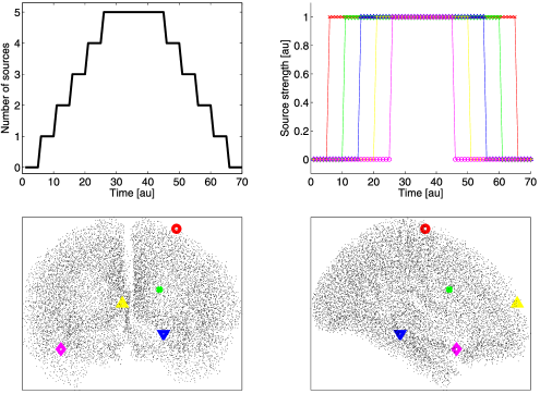
Figure 1: A sample dipole configuration generating one of the 100 data sets: in top left panel, the number of active sources as a function of time; in the top right panel, individual source waveforms; in the lower panels, the source locations and the grid points, randomly drawn from the uniform distribution in the brain.

The intensity of the dipole moment is kept fixed throughout the lifetime of each source, as shown in Figure 1 (although fixed intensity clearly does not mimic the actual behaviour of neural sources, we adopt this simple condition as it helps to provide a definite measure of the number of active sources at any time).

Noise is additive, zero-mean and Gaussian.

4.1.2 Point estimates for the multi-dipole configuration

The posterior distribution of a point process is a multidimensional object that is not easy to investigate and is hard to represent faithfully by point estimates, a problem which is well known in the multi-object tracking literature [see, e.g., Vo, Singh and Doucet (2005) for another setting in which a very similar problem arises]. At the same time, often in practical applications one is actually interested in point estimates; here, we are particularly interested in evaluating whether the particle filters provide good estimates of the dipole configuration that produced the synthetic data. We therefore propose a set of quantities that can be used for this purpose, bearing in mind that they are only low-dimensional projections of the actual output of the particle filter:

• The number of active sources can be represented via the marginal distribution for the number of dipoles, which can be computed from the approximation to the posterior density as

  $$P(N_{t}=k|b_{1:t})=\sum_{i}w_{t}^{i}\delta_{k,N_{t}^{i}}.$$ (22)

• The location of the active sources can be represented via the intensity measure of the corresponding point process. This provides information about the dipole location which is highly suited to visual inspection; from the particle filter we get the following approximation to the intensity measure:

  $$p(r_{t}|b_{1:t})\simeq\sum_{i}w_{t}^{i}\sum_{k=1}^{N_{t}^{i}}\delta_{r_{t},r_{t}^{i,(k)}}.$$ (23)

  In our implementation this approximation is defined for all the locations on the grid, but not continuously over the entire volume.

• The direction and the intensity of the estimated dipoles, that is, the vectorial mark of the point process: one way to provide such information is to calculate the average dipole moment at each location, conditional on having a dipole at that location:

  $$E[q_{t}|r]=\sum_{i}w_{t}^{i}\sum_{k=1}^{N_{t}^{i}}q_{t}^{i,(k)}\delta_{r,r_{t}^{i,(k)}}.$$ (24)

We use the following procedure to obtain a “representative set” of dipoles from the approximated posterior distribution: [1.]

estimate the number of dipoles in the set by taking the mode of the posterior distribution (22);

find the $N$ highest peaks of the intensity measure (23): a peak is a grid point where the intensity measure is higher than that of its neighbours; we take these peaks as point estimates of the dipole locations;

for each estimated dipole location, the estimated dipole moment will be the average dipole moment at that location, as in (24). As an alternative to the optimization in step (2), we also tried a clustering approach based on a Gaussian mixture model augmented with a uniform component, devised to model possible outliers; in the simulations below, the two approaches produced essentially the same results (not shown). While these measures are only low-dimensional projections and cannot replace the rich information contained in the posterior distribution, we feel they capture the most important features relevant to the neuroscientist.

4.1.3 Discrepancy measures

Once this typical set has been estimated, the discrepancy between the estimated dipole set $\widehat{j}_{t}=\{\widehat{d}_{t}^{(1)},\ldots,\widehat{d}_{t}^{(\widehat{N}_{t})}\}$ and the target dipole set $j_{t}=\{d_{t}^{(1)},\ldots,d_{t}^{(N_{t}))}\}$ can be computed. However, measuring the distance between two point sets is a nontrivial task even in the simple case when the two sets contain the same number of points, and it becomes even more complicated when the two sets contain a different number of points. Furthermore, in the application under study the points also have marks, or dipole moments, which should be taken into account. In the following, we list several useful measures of discrepancy between the target and the estimated dipole configurations:

• Average distance from closest target (ADCT): At first we may be interested in answering this question: how far, on average, is the estimated dipole from any of the target dipoles? To answer this question, we can calculate the ADCT, defined as

  $$\operatorname{ADCT}(t)=\frac{1}{\widehat{N}_{t}}\sum_{k=1}^{\widehat{N}_{t}}\min_{j}\bigl{|}\widehat{r}_{t}^{(k)}-r_{t}^{(j)}\bigr{|},$$ (25)

  where $|\cdot|$ denotes the Euclidean norm.

• Symmetrized distance (SD): We may also want to incorporate in the distance measure the presence of undetected sources. To do this, we calculate a symmetrized version of the ADCT,

  $$\operatorname{SD}(t)=\frac{1}{\widehat{N}_{t}}\sum_{k=1}^{\widehat{N}_{t}}\min_{j}\bigl{|}\widehat{r}_{t}^{(k)}-r_{t}^{(j)}\bigr{|}+\frac{1}{{N}_{t}}\sum_{j=1}^{{N}_{t}}\min_{k}\bigl{|}\widehat{r}_{t}^{(k)}-r_{t}^{(j)}\bigr{|}.$$ (26)

• Optimal SubPattern assignment metric (OSPA): If two estimated dipoles are both close to the same target dipole, neither ADCT nor SD will notice it. The OSPA metric [Schuhmacher, Vo and Vo (2008)] overcomes this limitation by forcing a one-to-one correspondence between the estimated and the target dipoles; the OSPA metric is defined as

  $$\operatorname{OSPA}(t)=\cases{\displaystyle\min_{\pi\in\Pi_{\widehat{N}_{t},N_{t}}}\frac{1}{\widehat{N}_{t}}\sum_{k=1}^{\widehat{N}_{t}}\bigl{|}\widehat{r}_{t}^{(k)}-r_{t}^{(\pi(k))}\bigr{|},&\quad$\mbox{if }\widehat{N}_{t}\leq N_{t},$\vspace*{2pt}\cr\displaystyle\min_{\pi\in\Pi_{{N}_{t},\widehat{N}_{t}}}\frac{1}{{N}_{t}}\sum_{k=1}^{{N}_{t}}\bigl{|}\widehat{r}_{t}^{(\pi(k))}-r_{t}^{(k)}\bigr{|},&\quad$\mbox{if }\widehat{N}_{t}>N_{t},$}$$ (27)

  where $\Pi_{k,l}$ is the set of all permutations of $k$ elements drawn from $l$ elements. Note that this metric only calculates the discrepancy between the dipoles in the smaller set and the subset of dipoles in the larger set that has the smaller discrepancy with those in the smaller set.

• Widespread measure (WM): Finally, we want to combine discrepancies in the source location with discrepancies in the dipole moment. The following measure does this by replacing each dipole (both in the target dipole set and in the estimated dipole set) with a Gaussian-like function in the brain, centered at the dipole location, with fixed variance and height proportional to the dipole moment; the difference between the two spatial distributions is then integrated in the whole brain:

  $$\operatorname{WM}(t)=\int\Biggl{|}\Biggl{[}\sum_{k=1}^{\widehat{N}_{t}}\bigl{|}\widehat{q}_{t}^{(k)}\bigr{|}\mathcal{N}\bigl{(}r;\widehat{r}_{t}^{(k)}\sigma\bigr{)}-\sum_{k=1}^{{N}_{t}}\bigl{|}{q}_{t}^{(k)}\bigr{|}\mathcal{N}\bigl{(}r;{r}_{t}^{(k)},\sigma\bigr{)}\Biggr{]}\Biggr{|}\,dr,$$ (28)

  where the integral must in practice be approximated by numerical methods.

4.1.4 Results

We ran the Resample-Move particle filter on the 100 synthetic data sets described at the beginning of this section. We also ran a bootstrap filter on the same data to evaluate its ability to sample the Static model’s posterior. In addition, we ran both a standard bootstrap and an improved filter, as described in the previous section, implementing the Random-Walk model.

All filters were run with 10,000 particles. In addition, in order to compare the performances for approximately equal computational cost, we ran both the Resample-Move filter and the improved filter for the Random-Walk model with 500 particles. All filters were run with the same parameter values: the standard deviation of the Gaussian prior for the dipole moment was set to $\sigma_{q}=1$ nAm; the noise covariance matrix was diagonal, with the same value $\sigma_{\mathrm{noise}}^{2}$ for each channel and estimated from the first 5 time points. This was done in analogy with typical MEG experiments with external stimuli, where a pre-stimulus interval is typically used to estimate the noise variance.

We computed the discrepancy measures proposed in Section 4. The results are shown in Figure 2; the widespread measure provided results that are very similar to those of the OSPA metric, hence, for brevity it is not shown here. In Figure 3 we show the estimated number of sources, the effective sample size, as given by equation (6), and the conditional likelihood as a function of time.

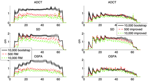
Figure 2: Simulation 1. Discrepancy measures for the Static model (left column) and the Random-Walk model (right column).

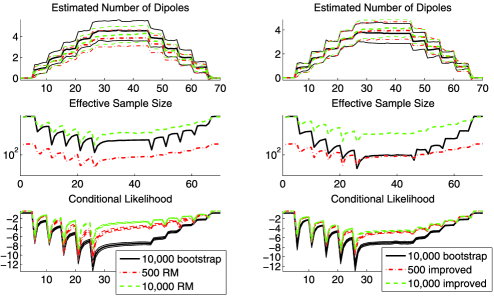
Figure 3: Simulation 1. Estimated number of sources, effective sample size and conditional likelihood for the Static model (left column) and the Random-Walk model (right column).

All the discrepancy measures indicate that the Resample-Move particle filter provides a substantial improvement over the bootstrap filter. The use of three different measures, in conjunction with the observation of the estimated number of sources in Figure 3, gives more insights about the qualitative nature of the improvements. First of all, the ADCT indicates that the dipoles estimated with the Resample-Move are on average much closer to the target sources; in addition, there is a rather small difference between the results obtained running the Resample-Move with 10,000 particles and with 500 particles. The average localization error is about 7 mm with the new model in contrast to the bootstrap particle filter which achieves an average localization error of 1.4 cm. The SD provides a slightly different result: there is more difference here between 500 and 10,000 particles; this is due to the fact that using a higher number of particles allows the algorithm to explore the state space better. In addition, the relatively small difference with the bootstrap filter here is due to the fact that the Resample-Move algorithm tends to slightly underestimate the number of sources, which is penalized by the SD. Finally, in terms of the OSPA measure, the Resample-Move provides a rather large improvement over the bootstrap: that the difference is so large is due to the fact that the bootstrap filter tends to overestimate the number of dipoles, in the proximity of a target dipole (as it is unable to update dipole locations and the likelihood strongly supports the presence of some additional signal source). This does not have a big impact on the ADCT, but is highly penalized by the OSPA. Observation of the ESS and of the conditional likelihood in Figure 3 strengthens the previous results. The Resample-Move algorithm maintains a higher ESS throughout the whole temporal window, in which the number of dipoles increases from zero to five and then returns to zero. The conditional likelihood further adds to the general evidence that the Resample-Move algorithm has better explored the state space whilst the bootstrap algorithm has missed a substantial part of the mass of the posterior. This plot also demonstrates that, as one would expect, better performance is obtained with a larger number of particles. However, with just 500 particles the Resample-Move algorithm provides better localisation performance than the bootstrap filter with 10,000 particles—as demonstrated by the various discrepancy measures.

Finally, we compare the performance of the Static model and the Random-Walk model. Noting that the bootstrap algorithm is unable to provide adequate inference for this model, as shown in Figure 2, we consider the proposed Resample-Move algorithm which is designed specifically to address the limitations of the simpler algorithm in this setting. The discrepancy measures indicate that the two models perform rather similarly in terms of average localization accuracy; this has to be regarded as a positive fact, since the localization accuracy of the Random-Walk model was already recognized as being satisfactory [Sorrentino et al. (2009)], and the Static model is in fact a model for which inference is harder. However, in most experimental conditions, the Random-Walk model is not believed to be as physiologically plausible as the Static model. Notably, in this synthetic experiment in which we know that the dipoles are actually static, we observe that the Static model leads to higher conditional likelihood than the random walk model. As in the context of Bayesian model selection, this implies that the data supports the Static model in preference to the Random-Walk model. However, some caution should be exercised in interpreting these results, as we are not dealing with the full Bayesian marginal likelihood: in both cases the true static parameters (noise variance, scale of random walk) have been fixed and so the time integral of these conditional likelihoods can only be interpreted as a marginal profile likelihood (it is not currently feasible to consider the penalisation of more complex models afforded by a fully Bayesian method in which the unknown parameters were marginalized out).

4.2 Simulation 2

We consider a simulated data set designed to mimic a real evoked response experiment, with the typical bell-shaped source time courses and real noise superimposed.

4.2.1 Generation of synthetic data

We generated the synthetic data shown in Figure 4. A first source (S1) in the central occipital area has peak strength at $30$ ms after the hypothetical stimulus; a second occipital but more lateral and ventral source (S2) peaks at $50$ ms; then one temporo-parietal source on the lateral surface (S3) and one parietal source on the medial surface (S4) peak at $80$ and $90$ ms, respectively, with a substantial temporal overlap. Noise free measurements were generated from the sources displayed in Figure 4 through the lead field matrix. In order to mimic a real-world data set, these noise-free data were added to the pre-stimulus signal from a real experiment, involving the same subject that was used to create the lead field matrix. The resulting noisy data are shown in the same figure.

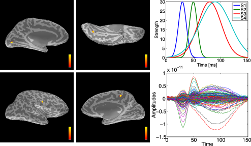
Figure 4: Simulation 2. Source locations (top row S1 and S2, bottom row S3 and S4), source time courses and generated noisy field.

4.2.2 Comparison with other methods

We compare the Resample-Move particle filter implementing the Static model with the particle filter implementing the Random-Walk model, as well as with three state-of-the-art methods for MEG source estimation:

• the recursively applied multiple signal classification (RAP-MUSIC) algorithm [Mosher, Lewis and Leahy (1992), Mosher and Leahy (1999)] is perhaps the most popular method for automatic estimation of current dipole parameters from MEG data, and is widely used as a reference method for both MEG and EEG dipole modeling [de Hoyos et al. (2012), Wu et al. (2012)]. After selection of a suitable number of components to identify a signal subspace, RAP-MUSIC computes an index at each point within the brain, representing the subspace correlation [Golub and Van Loan (1984)] between the leadfield at that point and the signal subspace. Peaks of this function are often used as point estimates of dipole locations;

• dynamic Statistical Parametric Mapping (dSPM) [Dale et al. (2000)] is a well-known method, whereby Tikhonov regularization is applied at each time point independently, and the so-obtained estimate of the electrical current distribution is divided by a location-dependent estimate of the noise variance; the resulting quantity, also named activity estimate, has a $t$-distribution under the null hypothesis of no activity. In the experiments below, we used the dSPM algorithm contained in the MNE software;

• $L_{1}L_{2}$ [Ou, Hämäläinen and Golland (2009), Gramfort, Kowalski andHämäläinen (2012)] is a spatio-temporal regularization method, whereby the penalty term has a mixed norm: an L1 norm in the spatial domain, encouraging sparsity of the estimated current distribution, and an L2 norm in the temporal domain, encouraging continuity of the source waveforms. In the experiments below, we used the $L_{1}L_{2}$ algorithm contained in the EMBAL Matlab toolbox (http://embal.gforge.inria.fr/).

We notice that the proposed comparison is necessarily a comparison of nonhomogeneous methods: while RAP-MUSIC is fundamentally a dipole localization method, $L_{1}L_{2}$ produces estimates of a continuous current distribution, and dSPM provides a statistical measure of activity; the particle filters, on the other hand, produce a dynamic approximation to the posterior distribution for a multiple current dipole model. For these reasons, a quantitative comparison resembling that of the previous section would be questionable and would fail to illustrate the fundamental differences between these methods. Therefore, in the following we provide a visual comparison of the main ouputs: the posterior intensity function for the particle filters; the subspace correlation index for RAP-MUSIC; the activity estimate for dSPM; the electrical current estimate for $L_{1}L_{2}$.

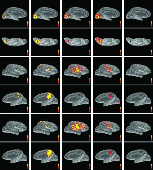
Figure 5: Simulation 2. Comparison of the maps produced by the Static model particle filter (first column), the Random-Walk model particle filter (second column), dSPM (third column), RAP-MUSIC (fourth column) and $L_{1}L_{2}$ (fifth column) at different time points: 30 ms (first row), 50 ms (second row), 75 ms (third and fourth rows), 90 ms (fifth and sixth rows). Black circles mark the locations of the true sources.

4.2.3 Results

In Figure 5 we show the results provided by the different methods at selected time points. Light and dark grey represent here the anatomical details, while color represents the estimated quantities, with values increasing from a threshold, red, to a maximum value, yellow. The color scale is different for each method: for the particle filters the threshold is $10^{-5}$ and the maximum is $0.1$; for dSPM the threshold is $5$ and the maximum is $15$; for RAP-MUSIC the threshold is $70$ and the maximum is $100$; for $L_{1}L_{2}$ the threshold is $1$ and the maximum is $30$. We notice that the correlation index provided by RAP-MUSIC is in fact not time-dependent; it is only for presentation purposes that we repeat the same figures at rows 3–4 and rows 5–6. The visualization of the brain is also worth a brief comment. The smooth brain surface in these images is indeed a computer representation in which the highly folded cortical surface is “inflated” in such a way that the activity in the sulci becomes easily visible. As a consequence, spatially adjacent volumes—for example, the portion of the cortex in two adjacent sulci—may be moved apart, therefore, the presence of multiple close-by peaks or blobs in these images is most often an artefact due to the visualization, rather than an actual multi-modality of the three-dimensional spatial distribution of the displayed quantity.

At $t=30$ ms, source 1 is recovered by all methods, the $L_{1}L_{2}$ solution being only slightly more superficial than the actual source; this happens despite the use of the same depth weighting method proposed in Lin et al. (2006) and described earlier in this paper. A direct comparison of the Static model with the Random-Walk model illustrates that the Static model tends to produce sparser probability maps: this is due to the Resample-Move algorithm being able to accumulate information on the source location with time. At $t=50$ ms, source 2 is correctly recovered by all methods, except $L_{1}L_{2}$; $L_{1}L_{2}$ does not produce any detectable output in the ventral area where source 2 is. In fact, we were able to estimate this source with $L_{1}L_{2}$ by modifying the value of the regularization parameter, but this came at the cost of making the solution at all time points notably less sparse, and much more similar to the one provided by dSPM. At $t=75$ ms, source 3 is recovered by all methods, with $L_{1}L_{2}$ providing a particularly accurate and sparse solution. However, source 4 is not recovered by $L_{1}L_{2}$ nor by dSPM; tweaking the parameters did not work for either method. On the other hand, the subspace correlation computed by RAP-MUSIC does have a local maximum around source 4, but its value of about 0.8 is not “close to 1,” hence, whether source 4 will be detected depends on the subjective choice of a threshold. The same comment applies to $t=90$ ms, where, in addition, we notice that, as already noted, the Static model implemented in the Resample-Move particle filter produces a more focal posterior map as time goes on, as a consequence of the accumulation of information on the source, while the Random-Walk model does not.

5 Application to real data

We applied the Resample-Move algorithm to real MEG recordings which were obtained during stimulation of a large nerve in the arm. This choice is motivated by the fact that the neural response to this type of somatosensory stimulation is relatively simple and rather well understood [Mauguiere et al. (1997)], and therefore allows a meaningful assessment of performance.

5.1 Experimental data

We used data from a Somatosensory Evoked Fields (SEFs) mapping experiment. The recordings were performed after informed consent was obtained, and had prior approval by the local ethics committee. Data were acquired with a 306-channel MEG device (Elekta Neuromag Oy, Helsinki, Finland) comprising 204 planar gradiometers and 102 magnetometers in a helmet-shaped array. The left median nerve at the wrist was electrically stimulated at the motor threshold with an interstimulus interval randomly varying between 7.0 and 9.0 s. The MEG signals were filtered to 0.1–200 Hz and sampled at 1000 Hz. Electrooculogram (EOG) was used to monitor eye movements that might produce artefacts in the MEG recordings; trials with EOG or MEG exceeding 150 mV or 3 pT/cm, respectively, were excluded and 84 clean trials were averaged. To reduce external interference, the signal space separation method [Taulu, Kajola and Simola (2004)] was applied to the average. A 3D digitizer and four head position indicator coils were employed to determine the position of the subject’s head within the MEG helmet with respect to anatomical MRIs obtained with a 3-Tesla MRI device (General Electric, Milwaukee, USA).

5.2 Results

The Resample-Move particle filter implementing the Static model was applied to the MEG recordings; for the sake of comparison, we also applied the particle filter based on the Random-Walk model and the conditional sampling, as well as dSPM, RAP-MUSIC and $L_{1}L_{2}$, the methods already used and briefly described in simulation 2. Both particle filters were run with the same parameter values. The standard deviation of the Gaussian prior for the dipole moment was set to $\sigma_{q}=50$ nAm, which is a physiologically plausible value; varying the value of this parameter did not qualitatively alter the reconstructions obtained. The noise covariance matrix was diagonal, the diagonal entries assuming either of two values, one for gradiometers and one for magnetometers; these values were obtained by averaging, across homogeneous channels, the channel-specific estimates of the standard deviation obtained from the pre-stimulus interval.

Figure 6 illustrates the localization provided by the five methods. We show snapshots at three time points. The very first response in the primary somatosensory area SI, at 25 ms, is localized by both the Static and the Random-Walk particle filters in a very similar way. The correlation index in RAP-MUSIC—which we recall is not time varying—clearly has a peak around the same location; the $L_{1}L_{2}$ activity estimate is slightly more superficial but still very close, while the dSPM estimate is rather widespread and indicates activity in slightly more frontal areas. At time $t=50$ ms after stimulus, the Static and the Random-Walk model are showing the same behaviour already observed in simulation 2: as the SI area has been active for the past 25 ms, the posterior map of the Static model is much more concentrated now, having accumulated information on the source location; the Random-Walk model indicates activity in the same area but provides a more blurred image. The estimate of dSPM is now closer to the probability maps provided by the two filters, while $L_{1}L_{2}$ does not show significant changes from the previous snapshot. At time $t=85$ ms, finally, we observe more activation in SI, and the additional activity in the ipsilateral and contralateral SII: observing the posterior maps provided by the Static model we observe, as in Mauguiere et al. (1997), that the contralateral SII activation is more frontal than the ipsilateral SII activation. The Random-Walk model provides, again, more blurred images. The dSPM estimate is again more widespread. RAP-MUSIC has local maxima around 0.85 in a similar area as the particle filters for the right hemisphere, while there is a slight disagreement on the left hemisphere; finally, the source distribution in $L_{1}L_{2}$ is not much changed on the right hemisphere, while on the left hemisphere it provides a slightly more posterior localization with respect to the one provided by the particle filter.

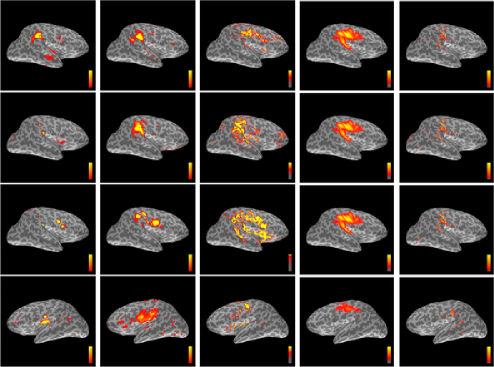
Figure 6: SEF data. Comparison of the maps produced by the Static model particle filter (first column), the Random-Walk model particle filter (second column), dSPM (third column), RAP-MUSIC (fourth column) and $L_{1}L_{2}$ (fifth column) at different time points: 25 ms (first row), 50 ms (second row), 85 ms (right hemisphere on the third row, left hemisphere on the fourth row).

In Figure 7 we show the cumulative marginal likelihood (7) and the effective sample size for the two particle filters. While the effective sample size produces rather similar results for the two models, the marginal likelihood indicates that after approximately $t=60$ ms the Static model provides higher likelihood than the Random-Walk model. Importantly, the cumulative likelihood at time $t$ is the likelihood of the whole time series up to time $t$. The fact that the difference between the two models tends to increase with time indicates that, as more data are gathered, the Static model is increasingly preferentially supported by the measurements. The ratio of the two likelihoods at the terminal time point indicates that the whole time series is several orders of magnitude more likely under the Static model than under the Random-Walk model, thus providing confirmation that the Static model is a much better representation of the underlying neurophysiological processes than the Random-Walk model. An additional point that deserves to be highlighted here is that not only are the probability maps provided by the Static model sparser than those provided by the Random-Walk, but also (as one might reasonably expect) they show less temporal variation. To illustrate this point, in Figure 8 we show two maps that have been obtained by integrating over time the dynamic probability maps provided by the Static and the Random-Walk filters: while the Static model has high probability in few small areas and negligible probability elsewhere, the Random-Walk model provides a flatter image, with rather homogeneous probability values in a larger area, a consequence of the fact that the Random-Walk model attaches a large part of its posterior probability mass to dipoles which move around the brain.

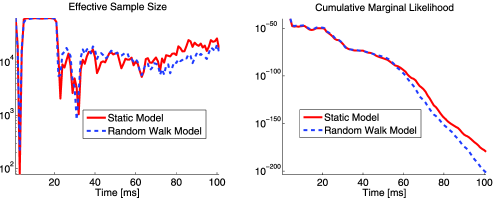
Figure 7: The effective sample size and the marginal likelihood, as obtained with the Static and the Random-Walk model with the SEF data.

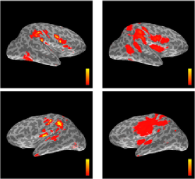
Figure 8: Time-integrated probability maps: the Static model (left column) exhibits less temporal variation than the Random-Walk model (right column).

As we run several independent realizations of the filters with the same parameter values and 100,000 particles, we observed that for $t>75$ ms not all the runs provide exactly the same estimates. While in the majority of the runs the mode of the posterior distribution consistently presents the source configuration depicted in Figure 6, in approximately 10% of the runs the ipsi-lateral and contra-lateral SII sources are replaced with a pair of sources in between the two hemispheres, one at the top in the motor area and one rather deep and central; the two SII areas are still represented in the posterior distribution, but with slightly lower mass, and may not appear in low-dimensional summaries of the posterior. As noted previously, accurately summarising high-dimensional multi-object posteriors is known to be a rather difficult problem. Finally, we note that if too small a sample size was employed, then we found that the quality of the approximation of the posterior could deteriorate to the point that the posterior did not contain mass in a neighbourhood of the configuration shown in Figure 6. Naturally, sample-based approximations to high-dimensional distributions fail to accurately capture the important features of those distributions if the sample is too small. In the case of a sample of size 10,000 we observed this failure mode in less than 10% of the runs. In practice, such a phenomenon should be easily detected by replicating the estimation procedure a number of times.

6 Discussion

In this study we have presented a new state-space model for dynamic inference on current dipole parameters from MEG data with particle filtering. The model has been devised to reflect the common neurophysiological interpretation of a current dipole as the activity of a small patch of cortex: the number of dipoles is time-varying, as dipoles can appear and disappear, and dipole locations are fixed during the dipole life time. Standard sequential Monte Carlo algorithms are not well suited to “filtering” of static parameters; for the same reasons simple sequential importance resampling is not able to efficiently approximate the posterior distributions associated with these near-static objects. We have developed a Resample-Move type algorithm with carefully designed proposal distributions which are appropriate for inference in this type of model.

We have used synthetic data to show that the average localization error provided by the Resample-Move algorithm is close to 5 mm, that is, the average grid spacing, even when the data are produced by five simultaneous dipoles. In addition, the effective sample size remains high even when the filter explores the high-dimensional parameter space of five dipoles, consistent with a good approximation of the posterior distribution. Although the quality of the approximation naturally depends on the sample size, we demonstrated good results can be obtained with a realistic computational cost. Finally, comparison of the conditional likelihood of our Static dipole model with that of a Random-Walk model indicates that the proposed method is actually capable of providing a better explanation of the data.

We have used a second simulation study to assess the localization capability of the particle filter in comparison with dSPM, RAP-MUSIC and $L_{1}L_{2}$. The activity maps showed that both particle filters were able to identify all the four sources in the simulation, while dSPM and $L_{1}L_{2}$ missed at least one, and RAP-MUSIC provided local peaks but with low intensity for one source. In addition, comparison of the probability maps provided by the Static and the Random-Walk models shows that the Static model coherently accumulates information on the source and provides more focal maps with time, while the Random-Walk does not.

Application of the proposed method to an experimental data set has produced similar results: the effective sample size and the conditional likelihood remain high throughout the whole time series; the posterior probability maps are well in accordance with what is understood to be the usual brain response to median nerve stimulation. The Static model leads to physiologically-interpretable output which is consistent with the biomedical understanding of the dipole model. We did not observe the type of artefacts found with the Random-Walk model in which dipoles slowly moved across the brain surface when using this model.

Future research will concentrate on increasing the number of samples and decreasing the computational time. Implementation on GPUs should provide a viable way to reduce the computational time exploiting massive parallelization and given performance improvements observed in similar settings [Lee et al. (2010)], thereby facilitating real-time implementation. This together with the bounded per-iteration computational cost of the filtering algorithm is a significant motivation of the approach. Improving the efficiency of the MCMC step is also of interest. Other possible interesting research directions include the use of smoothing [Briers, Doucet and Maskell (2010)] techniques and estimation of the static parameters (which were here fixed a priori using approaches prevalent in the literature) both online [Kantas et al. (2009)] and offline [Andrieu, Doucet and Holenstein (2010), Chopin, Jacob and Papaspiliopoulos (2011)], as well as generalization of the source model.

References

- Andrieu, Doucet and Holenstein (2010) {barticle}[mr] \bauthor\bsnmAndrieu, \bfnmChristophe\binitsC., \bauthor\bsnmDoucet, \bfnmArnaud\binitsA. and \bauthor\bsnmHolenstein, \bfnmRoman\binitsR. (\byear2010). \btitleParticle Markov chain Monte Carlo methods. \bjournalJ. R. Stat. Soc. Ser. B Stat. Methodol. \bvolume72 \bpages269–342. \biddoi=10.1111/j.1467-9868.2009.00736.x, issn=1369-7412, mr=2758115 \bptokimsref \endbibitem
- Briers, Doucet and Maskell (2010) {barticle}[mr] \bauthor\bsnmBriers, \bfnmMark\binitsM., \bauthor\bsnmDoucet, \bfnmArnaud\binitsA. and \bauthor\bsnmMaskell, \bfnmSimon\binitsS. (\byear2010). \btitleSmoothing algorithms for state-space models. \bjournalAnn. Inst. Statist. Math. \bvolume62 \bpages61–89. \biddoi=10.1007/s10463-009-0236-2, issn=0020-3157, mr=2577439 \bptokimsref \endbibitem
- Campi et al. (2008) {barticle}[mr] \bauthor\bsnmCampi, \bfnmC.\binitsC., \bauthor\bsnmPascarella, \bfnmA.\binitsA., \bauthor\bsnmSorrentino, \bfnmA.\binitsA. and \bauthor\bsnmPiana, \bfnmM.\binitsM. (\byear2008). \btitleA Rao–Blackwellized particle filter for magnetoencephalography. \bjournalInverse Problems \bvolume24 \bpages025023, 15. \biddoi=10.1088/0266-5611/24/2/025023, issn=0266-5611, mr=2408560 \bptokimsref \endbibitem
- Campi et al. (2011) {barticle}[pbm] \bauthor\bsnmCampi, \bfnmC.\binitsC., \bauthor\bsnmPascarella, \bfnmA.\binitsA., \bauthor\bsnmSorrentino, \bfnmA.\binitsA. and \bauthor\bsnmPiana, \bfnmM.\binitsM. (\byear2011). \btitleHighly automated dipole estimation (HADES). \bjournalComput. Intell. Neurosci. \bvolume2011 \bpages982185. \biddoi=10.1155/2011/982185, issn=1687-5273, pmcid=3061326, pmid=21437232 \bptokimsref \endbibitem
- Carpenter, Clifford and Fearnhead (1999) {barticle}[author] \bauthor\bsnmCarpenter, \bfnmJ.\binitsJ., \bauthor\bsnmClifford, \bfnmP.\binitsP. and \bauthor\bsnmFearnhead, \bfnmP.\binitsP. (\byear1999). \btitleAn improved particle filter for non-linear problems. \bjournalIEE Proceedings Radar, Sonar & Navigation \bvolume146 \bpages2–7. \bptokimsref \endbibitem
- Chopin (2004) {barticle}[mr] \bauthor\bsnmChopin, \bfnmNicolas\binitsN. (\byear2004). \btitleCentral limit theorem for sequential Monte Carlo methods and its application to Bayesian inference. \bjournalAnn. Statist. \bvolume32 \bpages2385–2411. \biddoi=10.1214/009053604000000698, issn=0090-5364, mr=2153989 \bptokimsref \endbibitem
- Chopin, Jacob and Papaspiliopoulos (2011) {bmisc}[author] \bauthor\bsnmChopin, \bfnmN.\binitsN., \bauthor\bsnmJacob, \bfnmP.\binitsP. and \bauthor\bsnmPapaspiliopoulos, \bfnmO.\binitsO. (\byear2011). \bhowpublishedSMC2: An efficient algorithm for sequential analysis of state-space models. Available at arXiv:\arxivurl1101.1528. \bptokimsref \endbibitem
- Cohen and Cuffin (1983) {barticle}[pbm] \bauthor\bsnmCohen, \bfnmD.\binitsD. and \bauthor\bsnmCuffin, \bfnmB. N.\binitsB. N. (\byear1983). \btitleDemonstration of useful differences between magnetoencephalogram and electroencephalogram. \bjournalElectroencephalogr. Clin. Neurophysiol. \bvolume56 \bpages38–51. \bidissn=0013-4694, pmid=6190632 \bptokimsref \endbibitem
- Dale, Fischl and Sereno (1999) {barticle}[pbm] \bauthor\bsnmDale, \bfnmA. M.\binitsA. M., \bauthor\bsnmFischl, \bfnmB.\binitsB. and \bauthor\bsnmSereno, \bfnmM. I.\binitsM. I. (\byear1999). \btitleCortical surface-based analysis. I. Segmentation and surface reconstruction. \bjournalNeuroimage \bvolume9 \bpages179–194. \biddoi=10.1006/nimg.1998.0395, issn=1053-8119, pii=S1053-8119(98)90395-0, pmid=9931268 \bptokimsref \endbibitem
- Dale et al. (2000) {barticle}[pbm] \bauthor\bsnmDale, \bfnmA. M.\binitsA. M., \bauthor\bsnmLiu, \bfnmA. K.\binitsA. K., \bauthor\bsnmFischl, \bfnmB. R.\binitsB. R., \bauthor\bsnmBuckner, \bfnmR. L.\binitsR. L., \bauthor\bsnmBelliveau, \bfnmJ. W.\binitsJ. W., \bauthor\bsnmLewine, \bfnmJ. D.\binitsJ. D. and \bauthor\bsnmHalgren, \bfnmE.\binitsE. (\byear2000). \btitleDynamic statistical parametric mapping: Combining fMRI and MEG for high-resolution imaging of cortical activity. \bjournalNeuron \bvolume26 \bpages55–67. \bidissn=0896-6273, pii=S0896-6273(00)81138-1, pmid=10798392 \bptokimsref \endbibitem
- de Hoyos et al. (2012) {barticle}[author] \bauthor\bparticlede \bsnmHoyos, \bfnmA.\binitsA., \bauthor\bsnmPortillo, \bfnmJ.\binitsJ., \bauthor\bsnmPortillo, \bfnmI.\binitsI., \bauthor\bsnmMarin, \bfnmP.\binitsP., \bauthor\bsnmMaestu, \bfnmF.\binitsF., \bauthor\bsnmPoch-Broto, \bfnmJ.\binitsJ., \bauthor\bsnmOrtiz, \bfnmT.\binitsT. and \bauthor\bsnmHernando, \bfnmAntonio\binitsA. (\byear2012). \btitleComparison and improvements of LCMV and MUSIC source localization techniques for use in real clinical environments. \bjournalJournal of Neuroscience Methods \bvolume205 \bpages312–323. \bptokimsref \endbibitem
- Del Moral (2004) {bbook}[mr] \bauthor\bsnmDel Moral, \bfnmPierre\binitsP. (\byear2004). \btitleFeynman–Kac Formulae: Genealogical and Interacting Particle Systems with Applications. \bpublisherSpringer, \blocationNew York. \biddoi=10.1007/978-1-4684-9393-1, mr=2044973 \bptokimsref \endbibitem
- Douc, Cappé and Moulines (2005) {binproceedings}[author] \bauthor\bsnmDouc, \bfnmR.\binitsR., \bauthor\bsnmCappé, \bfnmO.\binitsO. and \bauthor\bsnmMoulines, \bfnmE.\binitsE. (\byear2005). \btitleComparison of resampling schemes for particle filters. In \bbooktitleProceedings of the 4th International Symposium on Image and Signal Processing and Analysis I \bpages64–69. \bpublisherIEEE, \baddressZagreb, Croatia. \bptokimsref \endbibitem
- Doucet, Godsill and Andrieu (2000) {barticle}[author] \bauthor\bsnmDoucet, \bfnmA.\binitsA., \bauthor\bsnmGodsill, \bfnmS.\binitsS. and \bauthor\bsnmAndrieu, \bfnmC.\binitsC. (\byear2000). \btitleOn sequential Monte Carlo sampling methods for Bayesian filtering. \bjournalStatist. Comput. \bvolume10 \bpages197–208. \bptokimsref \endbibitem
- Doucet and Johansen (2011) {bincollection}[mr] \bauthor\bsnmDoucet, \bfnmA.\binitsA. and \bauthor\bsnmJohansen, \bfnmA. M.\binitsA. M. (\byear2011). \btitleA tutorial on particle filtering and smoothing: Fifteen years later. In \bbooktitleThe Oxford Handbook of Nonlinear Filtering \bpages656–704. \bpublisherOxford Univ. Press, \blocationOxford. \bidmr=2884612 \bptokimsref \endbibitem
- Geweke (1989) {barticle}[mr] \bauthor\bsnmGeweke, \bfnmJohn\binitsJ. (\byear1989). \btitleBayesian inference in econometric models using Monte Carlo integration. \bjournalEconometrica \bvolume57 \bpages1317–1339. \biddoi=10.2307/1913710, issn=0012-9682, mr=1035115 \bptokimsref \endbibitem
- Gilks and Berzuini (2001) {barticle}[mr] \bauthor\bsnmGilks, \bfnmWalter R.\binitsW. R. and \bauthor\bsnmBerzuini, \bfnmCarlo\binitsC. (\byear2001). \btitleFollowing a moving target—Monte Carlo inference for dynamic Bayesian models. \bjournalJ. R. Stat. Soc. Ser. B Stat. Methodol. \bvolume63 \bpages127–146. \biddoi=10.1111/1467-9868.00280, issn=1369-7412, mr=1811995 \bptokimsref \endbibitem
- Golub and Van Loan (1984) {bbook}[author] \bauthor\bsnmGolub, \bfnmG. H.\binitsG. H. and \bauthor\bparticleVan \bsnmLoan, \bfnmC. F.\binitsC. F. (\byear1984). \btitleMatrix Computation. \bpublisherJohns Hopkins Univ. Press, \blocationBaltimore. \bptokimsref \endbibitem
- Gordon, Salmond and Smith (1993) {barticle}[author] \bauthor\bsnmGordon, \bfnmN. J.\binitsN. J., \bauthor\bsnmSalmond, \bfnmD. J.\binitsD. J. and \bauthor\bsnmSmith, \bfnmA. F. M.\binitsA. F. M. (\byear1993). \btitleNovel approach to nonlinear/non-Gaussian Bayesian estimation. \bjournalIEE Proceedings F Radar and Signal Processing \bvolume140 \bpages107–113. \bptokimsref \endbibitem
- Gramfort, Kowalski and Hämäläinen (2012) {barticle}[author] \bauthor\bsnmGramfort, \bfnmA.\binitsA., \bauthor\bsnmKowalski, \bfnmM.\binitsM. and \bauthor\bsnmHämäläinen, \bfnmM.\binitsM. (\byear2012). \btitleMixed-norm estimates for the M/EEG inverse problem using accelerated gradient methods. \bjournalPhysics in Medicine and Biology \bvolume7 \bpages1937–1961. \bptokimsref \endbibitem
- Hämäläinen and Ilmoniemi (1984) {bmisc}[author] \bauthor\bsnmHämäläinen, \bfnmM.\binitsM. and \bauthor\bsnmIlmoniemi, \bfnmR. J.\binitsR. J. (\byear1984). \bhowpublishedInterpreting measured magnetic fields of the brain: Estimates of current distributions. Technical report, Helsinki Univ. Technology. \bptokimsref \endbibitem
- Hämäläinen and Ilmoniemi (1994) {barticle}[author] \bauthor\bsnmHämäläinen, \bfnmM.\binitsM. and \bauthor\bsnmIlmoniemi, \bfnmR. J.\binitsR. J. (\byear1994). \btitleInterpreting magnetic fields of the brain: Minimum norm estimates. \bjournalMedical & Biological Engineering & Computing \bvolume32 \bpages35–42. \bptokimsref \endbibitem
- Hämäläinen et al. (1993) {barticle}[author] \bauthor\bsnmHämäläinen, \bfnmM.\binitsM., \bauthor\bsnmHari, \bfnmR.\binitsR., \bauthor\bsnmKnuutila, \bfnmJ.\binitsJ. and \bauthor\bsnmLounasmaa, \bfnmO. V.\binitsO. V. (\byear1993). \btitleMagnetoencephalography: Theory, instrumentation and applications to non-invasive studies of the working human brain. \bjournalRev. Modern Phys. \bvolume65 \bpages413–498. \bptokimsref \endbibitem
- Jun et al. (2005) {barticle}[author] \bauthor\bsnmJun, \bfnmS. C.\binitsS. C., \bauthor\bsnmGeorge, \bfnmJ. S.\binitsJ. S., \bauthor\bsnmParè-Blagoev, \bfnmJ.\binitsJ., \bauthor\bsnmPlis, \bfnmS. M.\binitsS. M., \bauthor\bsnmRanken, \bfnmD. M.\binitsD. M., \bauthor\bsnmSchmidt, \bfnmD. M.\binitsD. M. and \bauthor\bsnmWood, \bfnmC. C.\binitsC. C. (\byear2005). \btitleSpatiotemporal Bayesian inference dipole analysis for MEG neuroimaging data. \bjournalNeuroImage \bvolume28 \bpages84–98. \bptokimsref \endbibitem
- Kantas et al. (2009) {bmisc}[author] \bauthor\bsnmKantas, \bfnmN.\binitsN., \bauthor\bsnmDoucet, \bfnmA.\binitsA., \bauthor\bsnmSingh, \bfnmS. S.\binitsS. S. and \bauthor\bsnmMaciejowski, \bfnmJ. M.\binitsJ. M. (\byear2009). \bhowpublishedAn overview of sequential Monte Carlo methods for parameter estimation in general state-space models. In 15th IFAC System Identification (SysId) Meeting Saint-Malo, France 774–785. \bptokimsref \endbibitem
- Kong, Liu and Wong (1994) {barticle}[author] \bauthor\bsnmKong, \bfnmA.\binitsA., \bauthor\bsnmLiu, \bfnmJ. S.\binitsJ. S. and \bauthor\bsnmWong, \bfnmW. H.\binitsW. H. (\byear1994). \btitleSequential imputations and Bayesian missing data problems. \bjournalJ. Amer. Statist. Assoc. \bvolume93 \bpages278–288. \bptokimsref \endbibitem
- Lee et al. (2010) {barticle}[author] \bauthor\bsnmLee, \bfnmA.\binitsA., \bauthor\bsnmYau, \bfnmC.\binitsC., \bauthor\bsnmGiles, \bfnmM. B.\binitsM. B., \bauthor\bsnmDoucet, \bfnmA.\binitsA. and \bauthor\bsnmHolmes, \bfnmC. C.\binitsC. C. (\byear2010). \btitleOn the utility of graphics card to perform massively parallel simulation with advanced Monte Carlo methods. \bjournalJ. Comput. Graph. Statist. \bvolume19 \bpages769–789. \bptokimsref \endbibitem
- Lin et al. (2006) {barticle}[author] \bauthor\bsnmLin, \bfnmF. H.\binitsF. H., \bauthor\bsnmWitzel, \bfnmT.\binitsT., \bauthor\bsnmAhlfors, \bfnmS. P.\binitsS. P., \bauthor\bsnmStufflebeam, \bfnmS. M.\binitsS. M., \bauthor\bsnmBelliveau, \bfnmJ. V.\binitsJ. V. and \bauthor\bsnmHamalainen, \bfnmM. S.\binitsM. S. (\byear2006). \btitleAssessing and improving the spatial accuracy in MEG source localization by depth-weighted minimum-norm estimates. \bjournalNeuroImage \bvolume31 \bpages160–171. \bptokimsref \endbibitem
- Long et al. (2006) {binproceedings}[author] \bauthor\bsnmLong, \bfnmC. J.\binitsC. J., \bauthor\bsnmPurdon, \bfnmP. L.\binitsP. L., \bauthor\bsnmTemeranca, \bfnmS.\binitsS., \bauthor\bsnmDesai, \bfnmN. U.\binitsN. U., \bauthor\bsnmHämäläinen, \bfnmM.\binitsM. and \bauthor\bsnmBrown, \bfnmE. N.\binitsE. N. (\byear2006). \btitleLarge scale Kalman filtering solutions to the electrophysiological source localization problem—a MEG case study. In \bbooktitleProceedings of the 28th IEEE EMBS Annual International Conference \bpages4532–4535. \bpublisherIEEE, \baddressNew York. \bptokimsref \endbibitem
- Long et al. (2011) {barticle}[mr] \bauthor\bsnmLong, \bfnmChristopher J.\binitsC. J., \bauthor\bsnmPurdon, \bfnmPatrick L.\binitsP. L., \bauthor\bsnmTemereanca, \bfnmSimona\binitsS., \bauthor\bsnmDesai, \bfnmNeil U.\binitsN. U., \bauthor\bsnmHämäläinen, \bfnmMatti S.\binitsM. S. and \bauthor\bsnmBrown, \bfnmEmery N.\binitsE. N. (\byear2011). \btitleState-space solutions to the dynamic magnetoencephalography inverse problem using high performance computing. \bjournalAnn. Appl. Stat. \bvolume5 \bpages1207–1228. \biddoi=10.1214/11-AOAS483, issn=1932-6157, mr=2849772 \bptokimsref \endbibitem
- Mauguiere et al. (1997) {barticle}[author] \bauthor\bsnmMauguiere, \bfnmF.\binitsF., \bauthor\bsnmMerlet, \bfnmI.\binitsI., \bauthor\bsnmForss, \bfnmN.\binitsN., \bauthor\bsnmVanni, \bfnmS.\binitsS., \bauthor\bsnmJousmaki, \bfnmV.\binitsV., \bauthor\bsnmAdeleine, \bfnmP.\binitsP. and \bauthor\bsnmHari, \bfnmR.\binitsR. (\byear1997). \btitleActivation of a distributed somatosensory cortical network in the human brain. A dipole modelling study of magnetic fields evoked by median nerve stimulation. Part I: Location and activation timing of SEF sources. \bjournalElectroencephalography and Clinical Neurophysiology \bvolume104 \bpages281–289. \bptokimsref \endbibitem
- Mosher and Leahy (1999) {barticle}[author] \bauthor\bsnmMosher, \bfnmJ. C.\binitsJ. C. and \bauthor\bsnmLeahy, \bfnmR. M.\binitsR. M. (\byear1999). \btitleSource localization using recursively applied and projected (RAP) MUSIC. \bjournalIEEE Trans. Signal Process. \bvolume47 \bpages332–340. \bptokimsref \endbibitem
- Mosher, Lewis and Leahy (1992) {barticle}[pbm] \bauthor\bsnmMosher, \bfnmJ. C.\binitsJ. C., \bauthor\bsnmLewis, \bfnmP. S.\binitsP. S. and \bauthor\bsnmLeahy, \bfnmR. M.\binitsR. M. (\byear1992). \btitleMultiple dipole modeling and localization from spatio-temporal MEG data. \bjournalIEEE Trans. Biomed. Eng. \bvolume39 \bpages541–557. \biddoi=10.1109/10.141192, issn=0018-9294, pmid=1601435 \bptokimsref \endbibitem