The central Blue Straggler population in four outer-halo globular clusters

Abstract

Using HST/WFPC2 data, we have performed a comparative study of the Blue Straggler Star (BSS) populations in the central regions of the globular clusters AM 1, Eridanus, Palomar 3, and Palomar 4. Located at distances $R_{GC}>50$ kpc from the Galactic Centre, these are (together with Palomar 14 and NGC 2419) the most distant clusters in the Halo. We determine their colour-magnitude diagrams and centres of gravity. The four clusters turn out to have similar ages (10.5-11 Gyr), significantly smaller than those of the inner-Halo globulars, and similar metallicities. By exploiting wide field ground based data, we build the most extended radial density profiles from resolved star counts ever published for these systems. These are well reproduced by isotropic King models of relatively low concentration. BSSs appear to be significantly more centrally segregated than red giants in all globular clusters, in agreement with the estimated core and half-mass relaxation times which are smaller than the cluster ages. Assuming that this is a signature of mass segregation, we conclude that AM 1 and Eridanus are slightly dynamically more evolved than Pal 3 and Pal 4.

1. Introduction

In the colour-magnitude diagram (CMD) of a globular cluster (GC), Blue Straggler Stars (BSSs) define a sub-population located along the main-sequence (MS) in a position brighter and bluer than the current MS-turnoff (TO). For this reason these objects are thought to be hydrogen burning stars more massive than a typical TO star. Two physical mechanisms are thought to be responsible for their formation: mass-transfer in a binary system (McCrea, 1964), and direct stellar collisions (Hills & Day, 1976). Since collisions are more frequent in regions of higher density, the relative importance of the different formation channels could depend on the environment (e.g., Fusi Pecci et al., 1992; Davies et al., 2004): BSSs in loose GCs might preferentially arise from mass-transfer activity in primordial binaries (hereafter MT-BSSs; Ferraro et al., 2006; Leigh et al., 2011a), while BSSs located in high density environments might mainly form from stellar collisions (hereafter COL-BSSs; Ferraro et al., 2004).

Discovered for the first time by Sandage (1953) in the external regions of the GC M3, it was with the advent of the Hubble Space Telescope (HST) and the 8-meter class telescopes that it became possible to search for BSSs in dense cluster cores (e.g. Paresce et al., 1991; Ferraro & Paresce, 1993; Clark et al., 2004). BSSs have been found in any properly imaged GC (Piotto et al., 2004) and they are studied also in dwarf spheroidal galaxies (Mapelli et al., 2007; Monelli et al., 2012).

Since the BSS formation mechanisms seems to be tightly connected with the cluster internal dynamics, these stars are commonly recognized as ideal test particles to investigate the impact of dynamics on stellar evolution in different environmental conditions (e.g. Bailyn, 1995; Sills & Bailyn, 1999; Moretti et al., 2008; Ferraro & Lanzoni, 2009). An interesting example comes from the discovery of two distinct sequences of BSSs in the core of M30 (Ferraro et al., 2009). The authors argued that each of the two sequences is populated by BSSs originated by one of the two formation channels, both triggered by the collapse of the cluster core a few Gyr ago. On the other side,  Knigge et al. (2009) suggest that most BSSs, even those found in cluster cores, come from binary systems (see also Leigh et al., 2011b). Nevertheless the parent binaries may themselves have been affected by dynamical encounters.

Systematic studies of the BSS populations in GCs have shown that in most cases their radial distribution is bimodal, with a high peak in the cluster centre, a trough at intermediate radii and a rising branch in the external regions (see e.g. Dalessandro et al., 2009, and references therein). Dynamical simulations (e.g. Sigurdsson et al., 1994; Mapelli et al., 2004, 2006; Lanzoni et al., 2007a, b) suggest that the observed shape of the BSS radial distribution depends on the relative contribution of COL-BSSs and the efficiency of the dynamical friction, that progressively segregates objects more massive than the average (as BSSs and their progenitors) towards the cluster centre. Very interesting exceptions are the cases of $\omega$ Centauri (Ferraro et al., 2006), NGC 2419 (Dalessandro et al., 2008) and Pal 14 (Beccari et al., 2011), where the BSS radial distribution is completely flat. This fact indicates that in these clusters the dynamical friction was not effective yet in segregating BSSs toward the centre of the potential well. Interestingly enough NGC 2419 and Pal 14 are among the most remote GCs in the Galaxy, lying at a distance from the Galactic centre $R_{GC}>50$ kpc.

We decided to extend the investigation to other four Galactic GCs (namely AM 1, Eridanus, Pal 3, Pal 4) located in the extreme outer-halo. In Section 2 we describe the data-set and reduction procedure. The CMD and the age estimate for each cluster are discussed in Section 2.1. The determination of the astrometric solutions and the cluster centres of gravity is presented in Section 2.2. The radial density profiles from resolved star counts and the estimates of the cluster structural parameters and characteristic time-scales are discussed in Section 3. Section 4 is devoted to the radial distribution of the BSS, while a summary is presented in Section 5.

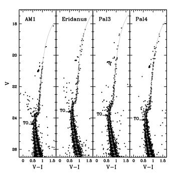
Figure 1.— (V,V-I) CMDs of the GCs AM 1, Eridanus, Pal 3, Pal 4. All the sampled stars are shown with black dots, while the location of the mean ridge line is shown with grey points. We fitted the CMD with isochrones from Dotter et al. (2008b, grey solid lines). The location of the MS-TO is also indicated.

2. The data set

Stetson et al. (1999, hereafter S99) published deep optical CMDs obtained with the Wide Field Planetary Camera 2 (WFPC2) on board the HST for Eridanus, Pal 3 and Pal 4. The core region of Eridanus was roughly centred on the WF3 chip of the WFPC2 mosaic, while Pal 3 and Pal 4 were centred on the PC chip. We refer to S99 (see also Harris et al., 1997) for a detailed description of data quality and reduction procedure. In brief, a standard DAOPHOTII (Stetson, 1987) Point Spread Function (PSF) fitting procedure, including ALLFRAME (Stetson, 1994), was adopted to obtain instrumental magnitudes and colours for all measurable stars in the WFPC2 fields. Here we adopted the S99 photometric catalogues of Pal 3, Pal 4 and Eridanus listing the $F555W$ and $F814W$ magnitudes of 2968, 4122 and 2340 stars, respectively.

AM 1 was observed with the WFPC2 in the $F555W$ and $F814W$ filters during Cycle 6 (GO-6512; PI Hesser). The observation log is described in Table 1 of Dotter et al. (2008a, hereafter D08). We retrieved the AM 1 images from the STScI archive and performed independent PSF fitting photometry. The PSF was modelled on each image using a number (between 40 and 80) of isolated and well sampled stars, adopting the PSF/DAOPHOTII routine. A first PSF fitting was then performed on every image using DAOPHOTII/ALLSTAR, while ALLFRAME was used to obtain a fine measure of the star magnitudes. For each star all the magnitudes were normalized to a reference frame and averaged together, and the photometric error was derived as the r.m.s. of the repeated measurements.

For homogeneity with the S99 reduction procedure, we used the colour terms in table 7 from Holtzman et al. (1995) to convert the instrumental ($F555W,F814W$) magnitudes to the standard Johnson V and Kron-Cousins I (hereafter V and I, respectively).

Figure 2.— The (V,V-I) CMDs of AM 1 (crosses), Eridanus (open squares), Pal 3 (open triangles), and Pal 4 (open circles) superimposed one to the other and aligned at the TO colour and magnitude, $(V-I)_{TO}$ and $V_{TO}$, respectively.

2.1. Colour-magnitude diagrams and age

The CMDs obtained for AM 1, Eridanus, Pal 3 and Pal 4 are shown in Figure 1 (see also figures 1–3 in S99). All the detected stars are shown as black dots, while the location of the mean ridge line obtained with a second order polynomial interpolation with a 2.5 sigma clipping rejection criterion is displayed with grey points. The high quality of the WFPC2 images allows us to properly sample the clusters’ stars from the Tip of the Red Giant Branch (RGB) down to $\sim 3$ mag below the MS-TO.

The solid line in Figure 1 shows the location of the best-fit theoretical isochrone from Dotter et al. (2008b) over-plotted on the CMDs of each cluster. We used the distance modulus and reddening from Harris (1996, 2010 edition), while we adopted metallicity [Fe/H]=–1.58 and –1.41 from Koch et al. (2009) and Koch & Côté (2010) for Pal 3 and Pal 4, respectively, [Fe/H]=–1.42 from S99 for Eridanus, and [Fe/H]=–1.5 from D08 for AM 1. With these parameters we obtain an absolute age of 10.5 Gyr for Eridanus and Pal 4, and 11 Gyr for Pal 3 and AM 1, confirming that these clusters are younger than the inner-halo GCs (S99 and D08).

The location of the TO, defined as the hottest point along the MS in the theoretical isochrone of each cluster, is also marked in Figure 1. This was used to compute the shifts in magnitude and colour that, after taking into account also the different distance moduli and reddenings, are necessary to co-add the four CMDs. The result is impressive (see Figure 2): the RGB morphologies of the four clusters are in full agreement and consistent with a small metallicity difference among their stellar populations. Indeed, the combined CMD mimics a highly homogeneous single-metallicity population. These results are in agreement with the study of S99 and D08, who find that these clusters are younger than M 3 by 1.5-2 Gyr, and they are homogeneous in terms of both age and metallicity.

Table 1Center of gravity of the target clusters.

Cluster	RA0	Dec0
AM 1	$03^{\rm h}55^{\rm m}02.5^{\rm s}$	$-49^{\circ}36\arcmin 53.2\arcsec$
Eridanus	$04^{\rm h}24^{\rm m}44.7^{\rm s}$	$-21^{\circ}11\arcmin 13.9\arcsec$
Pal 3	$10^{\rm h}05^{\rm m}31.6^{\rm s}$	$00^{\circ}04\arcmin 21.7\arcsec$
Pal 4	$11^{\rm h}29^{\rm m}16.5^{\rm s}$	$28^{\circ}58\arcmin 22.4\arcsec$

2.2. Astrometry and centre of gravity

The coordinates of the stars identified in each cluster have been converted from the “local” to the absolute astrometric system by using a well tested procedure adopted by our group for more than 10 years (see e.g. Lanzoni et al., 2010, and references therein). Since only a few (if any) primary astrometric standards can be found in the central region of GCs, we usually complement HST photometry with ground based wide-field imaging.

B- and R-band images of AM 1 where taken in December 2000 with the Wide Field Imager (WFI) at the MPE/ESO 2.2m telescope (66.B-0454(A); PI: Gallager). Pal 3, Pal 4 and Eridanus were observed in the $g$ and $r$ bands with MegaCam, the $\sim 1^{\circ}\times 1^{\circ}$ FoV CCD camera at the Canada-France-Hawaii Telescope (CFHT). We retrieved the bias-subtracted and flat-field corrected images from the CFHT Science Data Archive (Observing run ID: 2010AC06 for Pal 3 and Pal 4; 2009BC02 for Eridanus; PI Cote). We analysed the data following the procedure described in Section 2. We analysed only the few chips (from 2 to 4, depending on the location of the cluster centre in the FoV of each data-set) which allow us to sample the entire cluster radial extent. Notice that the tidal radius of the four clusters ranges between $\sim 2\arcmin$ and $\sim 5\arcmin$ (Harris, 1996). Unfortunately the ground based observations reach only the TO level and were not deep enough to properly sample the BSS region with an appropriate signal-to-noise ratio. For this reason we used this data set only to search for astrometric solutions and to supplement the HST data for the construction of the cluster projected density profiles from resolved star counts (see Sect. 3).

We used more than one hundred primary astrometric standard stars from the GSC2.3 catalogue in the cluster vicinity to derive an astrometric solution and obtain the absolute equatorial (RA and Dec) positions of the stars sampled in the ground based catalogues. Cross-correlations of the catalogues and astrometric solutions were calculated with CataXcorr, a code developed and maintained by Paolo Montegriffo at the INAF-Bologna Astronomical Observatory (see e.g. Lanzoni et al., 2010; Bellazzini et al., 2011). Finally, the positions of the stars in the WFPC2 data were transformed into the same celestial coordinate system by adopting $\sim 50$ stars in common with the ground based catalogues. The r.m.s. scatter of the final solution was $\sim 0.3\arcsec$ in both RA and Dec for the four clusters.

The centre of gravity ($C_{grav}$) of the four clusters is estimated as the barycenter of the resolved stars (see e.g. Lanzoni et al., 2010). In doing this an iterative procedure was adopted. The method estimates the centre by averaging the RA and Dec positions of all the stars contained within a circular area of a given radius and proceeds until convergence is reached. We performed this procedure using three different limiting radii and, at any given radius, using only stars with magnitudes brighter than $V_{TO}$, $V_{TO}+0.5$ mag and $V_{TO}+1$ mag. The final value of $C_{grav}$ is calculated as the average of the nine measures (see Table 1). The uncertainties both in RA and Dec are smaller than 1 arcsec for Eridanus and AM 1, while they increase to $\sim 2\arcsec$ for Pal 3 and Pal 4 because of the extremely low stellar density even in the core region of these clusters. Within the errors the new centres are in general good agreement with the ones listed by  Harris (1996).

Figure 3.— Observed surface density profiles in units of number of stars per square arcsecond. Star counts from the WFPC2 data are shown as solid circles, while those from ground based catalogues, normalised to the former, are shown as open diamonds. The solid line represents the King model that best fits the observed density profile over the entire cluster extent. Its characteristic parameters are labeled. The dashed horizontal line shows the adopted stellar density background, while the dotted-dashed vertical line indicates the cluster tidal radius ($r_{t}$). The lower panel shows the residuals between the observations and the fitted profile.

3. Radial density profiles

We used the photometric catalogues and the estimated values of $C_{grav}$ to calculate the projected radial density profile from resolved star counts for each cluster. We divided the entire sample into concentric annuli, each split into four subsectors (quadrants). The number of stars within each subsector was counted, and the star density was obtained by dividing these values by the corresponding subsector areas. The stellar density in each annulus was then obtained as the average of the subsector densities.

The star counts in the clusters’ central regions were performed using the stars with a magnitude $V<(V_{TO}+1)$ from the WFPC2 high-resolution imaging catalogues, while the stars sampled down to the TO were taken from the ground based data set for the external regions. Notice that the stars adopted to compute the density profile cover a very limited range of mass in both the HST and the ground based datasets, so that a single mass-model can be used to properly describe the observed profile (see next Section). The final density profiles of the program clusters are shown in Figure 3, where the star counts from ground based catalogues (open diamonds) have been normalised to the WFPC2 ones (solid circles) using at least two circular area in common between the two data sets. These are the most accurate and extended radial density profiles ever published for these GCs.

Table 2Age and structural parameters of the four GCs. Ages were estimated through the best-fit of theoretical isochrones. The uncertainties on the age are of the order of 0.2-0.3 Gyr. Cluster total masses have been computed from the observed total luminosities quoted by Harris (1996) and the mass-to-light ratios estimated by McLaughlin & van der Marel (2005) (an average value of 1.9 has been adopted for the mass-to-light ratio of Eridanus, which is not included in this latter work). The dimensionless potential, concentration, core and tidal radii and central mass density ($W_{0}$, $c$, $r_{c}$, $r_{t}$ and $\log(\rho_{0})$, respectively) are from the best-fit King models. The core relaxation time $\log(t_{rc})$ and half-mass relaxation time $\log(t_{rh})$ are computed following eq. (10) and (11) of Djorgovski (1993), respectively.

Cluster	Age	$\log(M_{cl})$	$W_{0}$	$c$	$r_{c}$	$r_{t}$	$\log(\rho_{0})$	$\log(t_{rc})$	$\log(t_{rh})$
	[Gyr]	$[M_{\odot}]$			[pc]	[pc]	$[M_{\odot}/\rm pc^{3}$]	[yr]	[yr]
AM1	11.0	4.10	5.60	1.16	5.99	95.12	0.48	9.02	$9.55$
Eridanus	10.5	4.26	5.00	1.03	6.35	77.01	0.06	9.32	$9.70$
Pal3	11.0	4.48	3.40	0.74	12.74	89.72	0.04	9.95	$9.95$
Pal4	10.5	4.62	3.60	0.77	12.59	93.77	0.18	9.96	$10.01$

3.1. King models and structural parameters

The derived density profiles allowed us to derive the clusters’ structural parameters through fitting isotropic King models (King, 1966). The background density was estimated from the outer data points. The best fit has been determined by $\chi^{2}$ minimization.

As shown in Figure 3, the observed profiles are very well reproduced by isotropic King models characterised by the quoted parameters, with $W_{0}$, $c$, $r_{c}$ and $r_{t}$ indicating the central dimensionless potential, the concentration, the core and tidal radii, respectively (see also Table 2; we adopted the distances quoted by Harris, 1996). These parameters have been used to estimate the core relaxation time ($t_{rc}$) and the half-mass relaxation time ($t_{rh}$) of the four clusters from equation (10) and (11) of Djorgovski (1993). We assumed the average stellar mass $\langle m_{\ast}\rangle=0.42M_{\odot}$ (Sollima et al., 2011) while the total cluster masses $M_{cl}$ have been derived from the observed total luminosity (Harris, 1996) and the mass-to-light ratios quoted by McLaughlin & van der Marel (2005, we adopted an average value of 1.9 for Eridanus, which is not included in that work). The resulting values of $t_{\rm rc}$ and $t_{rh}$ are shorter than the age of the clusters (Table 2). Hence, some degree of central mass segregation is expected in the program clusters. This result is at odds with what found in the two outer halo GCs previously investigated, NGC 2419 and Pal 14, whose $t_{rh}$ ($\sim 18$ and $\sim 20$ Gyr, respectively) are longer than the clusters’ ages ($\sim 12$ and $\sim 10.5$, respectively; see Dalessandro et al., 2009, and D08).

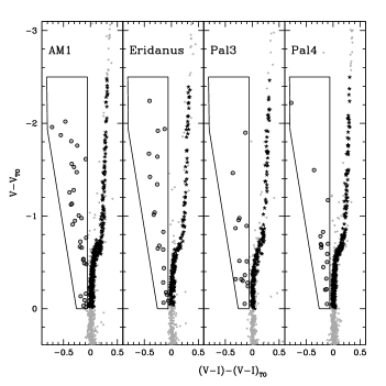
Figure 4.— Population selection in the four clusters. The bona-fide BSSs, located within the marked selection boxes, are shown as open circles. The reference population of RGB stars is marked with asterisks.

4. The BSS radial distribution

As demonstrated by previous results (see e.g. Ferraro et al., 2004; Carraro & Seleznev, 2011; Sanna et al., 2012; Salinas et al., 2012, and references therein), BSSs in most Galactic GCs are more centrally concentrated than normal stars. Since BSSs are more massive than the average, and since the half-mass relaxation time in those systems is much smaller than their age, this result is generally ascribed to the effect of dynamical friction and mass segregation (e.g. Mapelli et al., 2006).

The clusters studied in this paper contain a significant number of candidate BSSs (see Figure 2; see also Sandquist, 2005, hereafter S05). In order to investigate their radial distribution, the BSS populations have been selected in a homogeneous way in all clusters. We assumed the TO as the reference point and selected as bona-fide BSSs all the stars brighter than $V_{TO}$ and $3\times\sigma_{VI}$ bluer than $(V-I)_{TO}$, where $V_{TO}$ and $(V-I)_{TO}$ are, respectively, the magnitude and colour of the TO as defined in Section 2.1, while $\sigma_{VI}$ is the combined photometric uncertainty in the colour. The adopted selection boxes and the resulting bona-fide BSS samples are shown in Figure 4.

According to Ferraro et al. (1993), in order to study the radial distribution of BSSs, it is necessary to define a reference population which is expected to follow the cluster light distribution. Since the number of horizontal branch stars in these GCs is very low, we decided to adopt the RGB as the reference population. We selected as giants all the stars in the range of magnitude $V_{TO}>V>V_{TO}-2.5$, lying at a distance smaller than 3$\sigma$ from the mean ridge line (see asterisks in Figure 4), where $\sigma$ is the uncertainty associated with the mean ridge line (horizontal bars in Figure 1). This choice allows us to obtain a populous sample of reference stars in the same range of V magnitude, i.e., in the same condition of completeness as for the BSSs. The total number of BSSs and RGB stars in each cluster is listed in Table 3.

Table 3Number of BSSs and RGB stars selected in each cluster.

Cluster	NBSS	NRGB
AM 1	31	352
Eridanus	19	187
Pal 3	15	191
Pal 4	16	354

4.1. Cumulative radial distribution and population ratios

In Figure 5 we show the cumulative radial distribution of BSSs (solid lines) and RGB stars (dashed lines) as a function of the projected distance from the cluster centre ($r$) normalized to the core radius $r_{c}$ estimated in Section 3.1. A Kolmogorov-Smirnov test has been performed to check the probability that BSSs and RGB stars are extracted from the same parent distribution. Based on the probability values ($p$) obtained for each cluster and reported in Figure 5, we conclude that BSS are more concentrated than the RGB in AM 1 and Eridanus, while the result is inconclusive for Pal 3 and Pal 4.

As second step to investigate the radial distribution of BSSs in the four clusters, we calculated the ratio between the number of BSS (N_BSS) and that of RGB stars (N_RGB), counted in concentric annuli centred on the clusters’ $C_{grav}$. The radial distribution of N${}_{\rm BSS}/{\rm N}_{\rm RGB}$ in the four clusters is shown in Figure 6. Consistently with what was found above, BSSs appear to be systematically more centrally concentrated than RGB stars. It is important to emphasise that, because of the insufficient quality of the wide-field data, we are forced to limit our analysis to the region sampled by the HST observations, which do not reach the tidal radius of the program clusters. Thus, unfortunately we cannot characterise the full shape of the BSS radial distribution, and we are not able to conclude whether the distributions are bimodal or not. However this analysis demonstrates that dynamical friction was already effective in centrally segregating BSSs in the program clusters.

Figure 5.— Cumulative radial distributions of BBSs (solid lines) and RGB stars (dashed lines) as a function of their projected distance from the cluster centre normalised to the core radius ($r/r_{c}$), for each of the four clusters. The probability that the two populations are extracted from the same distribution is quoted in each panel.

Figure 6.— Relative frequency of BSS-to-RGB stars, as a function of the projected distance from the centre normalized to the core radius ($r/r_{c}$) for each of the four clusters.

4.2. The Minimum Spanning Tree

Given the relatively small number of BSSs, we applied the method of the Minimum Spanning Tree (MST; see Allison et al., 2009, and references therein) as an alternative test to evaluate the degree of BSS segregation. The MST is the unique set of straight lines (“edges”) connecting a given sample of points (“vertices”; in this case the star coordinates) without closed loops, such that the sum of the edge lengths is the minimum possible. Hence, the length of the MST is a measure of the compactness of a given sample of vertices. Cartwright & Whitworth (2004) showed that the degree of mass segregation in a star cluster can be measured by comparing the length of the MST of two populations with different average masses (see also Schmeja & Klessen, 2006). Notice that the MST method is independent of the catalogue astrometric accuracy and of any assumption about the cluster center. Moreover, it gives quantitative measures of both the degree of mass segregation and its associated significance.

Here we provide a detailed analysis of the segregation of BSSs with respect to RGB stars in the four program clusters, based on a recent modification of the MST method, where, instead of the direct sum of $n$ edges of length $e_{i}$, their geometric mean is used (Olczak et al., 2011):

$$\gamma_{\rm MST}=\left(\prod_{i=1}^{n}e_{i}\right)^{1/n}=\exp\left[\frac{1}{n}\sum_{i=1}^{n}\ln e_{i}\right].$$ (1)

Following equation (2), we have computed $\gamma_{\rm MST}^{\rm mass}$ for the most massive population (i.e., the observed samples of $n+1$ BSSs in each cluster). Then, we randomly extracted $m$ sets of $n+1$ objects from the reference population (the combination of the BSS and the RGB samples), and we computed their mean and standard deviation, $\bar{\gamma}_{\rm MST}^{\rm ref}$ and $\Delta{\gamma_{\rm MST}^{\rm ref}}$ respectively. Finally, the level of BSS segregation with respect to giant stars and its associated uncertainty have been estimated as:

$$\Gamma_{\rm MST}=\frac{\bar{\gamma}_{\rm MST}^{\rm ref}}{\gamma_{\rm MST}^{\rm mass}}\,,\\ \Delta{\Gamma_{\rm MST}}=\frac{\Delta{\gamma_{\rm MST}^{\rm ref}}}{\gamma_{\rm MST}^{\rm mass}}.$$ (2)

The geometrical mean has the very useful property of effectively damping contributions from extreme edge lengths, so that $\Gamma_{\rm MST}$ of a compact configuration of even a few stars will not be much affected by an “outlier”. Note that $\gamma_{\rm MST}$ has the dimension of a length, while $\Gamma_{\rm MST}$ is dimensionless. A value of $\Gamma_{\rm MST}=1$ is found if the two populations have the same radial distribution, while $\Gamma_{\rm MST}>1$ indicates the presence of mass segregation meaning a more concentrated distribution of massive stars compared to the reference population. In the latter case, the significance of mass segregation is provided by the value of $k$ for which $\Gamma_{\rm MST}-k\,\Delta{\Gamma_{\rm MST}}=1$.

Table LABEL:tab_mst lists the values of $\Gamma_{\rm MST}$ and the related $1\sigma$ uncertainties computed for the BSS populations in the four target clusters, and, for comparison, for NGC 2419 and Pal 14. In agreement with the results of Dalessandro et al. (2008) and Beccari et al. (2011), we find that BSS and RGB stars share the same radial distribution in NGC 2419 and Pal 14 ($\Gamma_{\rm MST}\simeq 1$). Conversely, BSSs appear to be significantly more segregated than giant stars in the other four GCs. In particular, AM 1 and Eridanus show the highest level of mass segregation (with $\Gamma_{\rm MST}\simeq 1.7$), with high statistical significance ($2.5-3\sigma$). Pal 3 and Pal 4 show a slightly lower degree of BSS segregation ($\Gamma_{\rm MST}\simeq 1.5$), at the $\sim 2\sigma$ level.

Table 4Values of the MST tree ($\Gamma_{\rm MST}$) and its $1\sigma$ uncertainty ($\Delta{\Gamma_{\rm MST}}$) for the BSS in the four target clusters and for NGC 2419 and Pal 14.

Cluster	$\Gamma_{\rm MST}$	$\Delta{\Gamma_{\rm MST}}$
AM 1	1.71	0.23
Eridanus	1.69	0.27
Pal 3	1.56	0.27
Pal 4	1.53	0.29
NGC 2419	1.01	0.07
Pal 14	1.07	0.17

5. Summary

Using HST-WFPC2 data we studied the BSS population in the central regions of four Galactic halo GCs, namely AM 1, Eridanus, Pal 3 and Pal 4. These clusters, together with NGC 2419 and Pal 14, represent the entire group of GCs at $R_{GC}>50$ kpc.

A proper comparison of the derived CMDs with theoretical isochrones confirms the younger ages (10.5-11 Gyr) of these systems with respect to the inner-halo GCs (see Figure 1). The impressive similarity of their RGB morphology (Fig. 2) also indicates a small metallicity difference ($-1.41<$[Fe/H]$<-1.58$, depending on the cluster), in agreement with previous findings by S99 and D08.

By complementing HST data with wide-field catalogues from ground based imaging, we have derived the most extended radial density profiles from resolved star counts ever published for these clusters (Fig. 3). All profiles are well fit by isotropic King models with the structural parameters listed in Table 2.

Unluckily, the insufficient quality of the wide field catalogues did not allow us to study the BSS populations in the cluster outskirts and look for possible signatures of an external rising branch, similar to that found in most of the previously surveyed GCs (see Sanna et al., 2012, and references therein). We therefore limited the analysis to the area covered by the HST data. BSSs have been selected in a homogenous way in the four program clusters and their radial distribution has been compared to that of RGB stars, taken as a reference. We found that BSSs are significantly more centrally concentrated than giants in all four systems (see Figs. 5, 6 and Table LABEL:tab_mst). Since BSSs are assumed to be more massive than normal cluster stars, their higher central concentration is interpreted in terms of an effect of mass segregation. Indeed, the half-mass relaxation time of the four program GCs is found to be smaller than their age (see Table 2), thus indicating that dynamical friction has been already effective in segregating the most massive stars in the cores. By measuring the degree of mass segregation with the $\Gamma_{\mathrm{MST}}$ test, we conclude that AM 1 and Eridanus are the dynamically oldest systems in the group, while Pal 3 and Pal 4 are slightly less dynamically evolved, and NGC 2419 and Pal 14 show no signature of mass segregation yet (see also Dalessandro et al., 2008; Beccari et al., 2011). The results shown in this paper once more indicate that, indeed, BSSs represent the ideal population to investigate the dynamical state of dense stellar systems.

References

- Allison et al. (2009) Allison, R. J., Goodwin, S. P., Parker, R. J., et al. 2009, MNRAS, 395, 1449
- Bailyn (1995) Bailyn, C. D. 1995, ARA&A, 33, 133
- Beccari et al. (2011) Beccari, G., Sollima, A., Ferraro, F. R., et al. 2011, ApJ, 737, L3
- Bellazzini et al. (2011) Bellazzini, M., Beccari, G., Oosterloo, T. A., et al. 2011, A&A, 527, A58
- Binney & Tremaine (1987) Binney, J., & Tremaine, S. 1987, Princeton, NJ, Princeton University Press, 1987, 747 p.,
- Caliskan et al. (2011) Caliskan, S., Christlieb, N., & Grebel, K. E. 2011, arXiv:1110.5151
- Carraro & Seleznev (2011) Carraro, G., & Seleznev, A. F. 2011, MNRAS, 412, 1361
- Cartwright & Whitworth (2004) Cartwright, A., & Whitworth, A. P. 2004, MNRAS, 348, 589
- Clark et al. (2004) Clark, L. L., Sandquist, E. L., & Bolte, M. 2004, AJ, 128, 3019
- Dalessandro et al. (2008) Dalessandro, E., Lanzoni, B., Ferraro, F. R., Vespe, F., Bellazzini, M., & Rood, R. T. 2008, ApJ, 681, 311
- Dalessandro et al. (2009) Dalessandro, E., Beccari, G., Lanzoni, B., Ferraro, F. R., Schiavon, R., & Rood, R. T. 2009, ApJS, 182, 509
- Davies et al. (2004) Davies, M. B., Piotto, G., & de Angeli, F. 2004, MNRAS, 349, 129
- Djorgovski (1993) Djorgovski, S. 1993, Structure and Dynamics of Globular Clusters, 50, 373
- Dotter et al. (2008a) Dotter, A., Sarajedini, A., & Yang, S.-C. 2008a, AJ, 136, 1407 (D08)
- Dotter et al. (2008b) Dotter, A., Chaboyer, B., Jevremović, D., et al. 2008b, ApJS, 178, 89
- Ferraro et al. (1993) Ferraro, F. R., Pecci, F. F., Cacciari, C., et al. 1993, AJ, 106, 2324
- Ferraro & Paresce (1993) Ferraro, F. R., & Paresce, F. 1993, AJ, 106, 154
- Ferraro et al. (2004) Ferraro, F. R., Beccari, G., Rood, R. T., et al. 2004, ApJ, 603, 127
- Ferraro et al. (2006) Ferraro, F. R., Sollima, A., Rood, R. T., Origlia, L., Pancino, E., & Bellazzini, M. 2006, ApJ, 638, 433
- Ferraro et al. (2009) Ferraro, F. R., Beccari, G., Dalessandro, E., et al. 2009, Nature, 462, 1028
- Ferraro & Lanzoni (2009) Ferraro, F. R., & Lanzoni, B. 2009, Revista Mexicana de Astronomia y Astrofisica Conference Series, 37, 62
- Frank et al. (2012) Frank, M. J., Hilker, M., Baumgardt, H., et al. 2012, arXiv:1205.2693
- Fusi Pecci et al. (1992) Fusi Pecci, F., Ferraro, F. R., Corsi, C. E., Cacciari, C., & Buonanno, R. 1992, AJ, 104, 1831
- King (1966) King, I. R. 1966, AJ, 71, 64
- Knigge et al. (2009) Knigge, C., Leigh, N., & Sills, A. 2009, Nature, 457, 288
- Koch et al. (2009) Koch, A., Côté, P., & McWilliam, A. 2009, A&A, 506, 729
- Koch & Côté (2010) Koch, A., & Côté, P. 2010, A&A, 517, A59
- Harris (1996) Harris, W.E. 1996, AJ, 112, 1487.
- Harris et al. (1997) Harris, W. E., Bell, R. A., Vandenberg, D. A., et al. 1997, AJ, 114, 1030
- Hills & Day (1976) Hills, J. G., & Day, C. A. 1976, Astrophys. Lett., 17, 87
- Holtzman et al. (1995) Holtzman, J. A., Burrows, C. J., Casertano, S., et al. 1995, PASP, 107, 1065
- Lanzoni et al. (2007a) Lanzoni, B., Dalessandro, E., Ferraro, F. R., Mancini, C., Beccari, G., Rood, R. T., Mapelli, M., & Sigurdsson, S. 2007a, ApJ, 663, 267
- Lanzoni et al. (2007b) Lanzoni, B., et al. 2007b, ApJ, 663, 1040
- Lanzoni et al. (2010) Lanzoni, B., Ferraro, F. R., Dalessandro, E., et al. 2010, ApJ, 717, 653
- Leigh et al. (2011a) Leigh, N., Sills, A., & Knigge, C. 2011a, MNRAS, 416, 1410
- Leigh et al. (2011b) Leigh, N., Sills, A., & Knigge, C. 2011b, MNRAS, 415, 3771
- Mapelli et al. (2004) Mapelli, M., Sigurdsson, S., Colpi, M., et al. 2004, ApJ, 605, L29
- Mapelli et al. (2006) Mapelli, M., Sigurdsson, S., Ferraro, F. R., Colpi, M., Possenti, A., & Lanzoni, B. 2006, MNRAS, 373, 361
- Mapelli et al. (2007) Mapelli, M., Ripamonti, E., Tolstoy, E., et al. 2007, MNRAS, 380, 1127
- McCrea (1964) McCrea, W. H. 1964, MNRAS, 128, 147
- McLaughlin & van der Marel (2005) McLaughlin, D. E., & van der Marel, R. P. 2005, ApJS, 161, 304
- Momany et al. (2007) Momany, Y., Held, E. V., Saviane, I., et al. 2007, A&A, 468, 973
- Monelli et al. (2012) Monelli, M., Cassisi, S., Mapelli, M., et al. 2012, ApJ, 744, 157
- Moretti et al. (2008) Moretti, A., de Angeli, F., & Piotto, G. 2008, A&A, 483, 183
- Olczak et al. (2011) Olczak, C., Spurzem, R., & Henning, T. 2011, A&A, 532, A119
- Paresce et al. (1991) Paresce et al. 1991, Nature, 352, 297
- Piotto et al. (2004) Piotto, G., De Angeli, F., King, I. R., et al. 2004, ApJ, 604, L109
- Salinas et al. (2012) Salinas, R., Jílková, L., Carraro, G., Catelan, M., & Amigo, P. 2012, MNRAS, 421, 960
- Sandage (1953) Sandage, A. R. 1953, AJ, 58, 61
- Sandquist (2005) Sandquist, E. L. 2005, ApJ, 635, L73
- Sanna et al. (2012) Sanna, N., Dalessandro, E., Lanzoni, B., et al. 2012, MNRAS, 2579
- Schmeja & Klessen (2006) Schmeja, S., & Klessen, R. S. 2006, A&A, 449, 151
- Sigurdsson et al. (1994) Sigurdsson, S., Davies, M. B., & Bolte, M. 1994, ApJ, 431, L115
- Sills & Bailyn (1999) Sills, A., & Bailyn, C. D. 1999, ApJ, 513, 428
- Sollima et al. (2011) Sollima, A., Martinez-Delgado, D., Valls-Gabaud, D., & Pe narrubia, J. 2011, ApJ, 726, 47 (S11)
- Stetson (1987) Stetson, P. B. 1987, PASP, 99, 191
- Stetson (1994) Stetson, P. B. 1994, PASP, 106, 250
- Stetson et al. (1999) Stetson, P. B., Bolte, M., Harris, W. E., et al. 1999, AJ, 117, 247 (S99)
- Zaggia et al. (1997) Zaggia, S. R., Piotto, G., & Capaccioli, M. 1997, A&A, 327, 1004